Systematic equity allocation across countries for dollar-based investors

Jupyter Notebook

This post demonstrates that country allocation with macroeconomic factors can materially enhance the returns on international equity portfolios in dollar terms. We identify a range of economic developments that, according to standard theory and in conjunction with market inattention, should predict the outperformance of countries either through exchange rate appreciation or higher local-currency equity returns. These developments are captured in backtestable economic factor scores, built from point-in-time macro-quantamental indicators. To select and combine these factors into trading signals without hindsight bias, we employ sequential machine learning. Empirical evidence based on 19 international markets shows highly significant predictive power and consistent material value arising from cross-country allocation alone. A simulation of U.S. dollar-based cross-country allocation of real money investment also reveals material long-term outperformance relative to an equally-weighted international portfolio or a U.S. portfolio.

The post below is based on Macrosynergy’s proprietary research. Please quote as “Costa, Michele and Sueppel, Ralph, ‘Systematic equity allocation across countries for dollar-based investors,’ Macrosynergy research post, August 2025.”

A Jupyter notebook for auditing and replicating the research results can be downloaded here. The notebook operation requires access to J.P. Morgan DataQuery to download data from JPMaQS. Everyone with DataQuery access can download data except for the latest months. Moreover, J.P. Morgan offers free trials on the complete dataset for institutional clients. An academic support program sponsors data sets for research projects.

Cross-country equity allocation: FX and equity risk

This post explains how to use macro trading factors to allocate equity positions across different currency areas, from the perspective of a U.S. dollar-based real-money investor. The goal is to predict differences in the dollar returns of international equity indexes and use macro factors to guide allocation. Unlike previous Macrosynergy posts, which focused on local-currency index futures and a leveraged investor’s perspective (Cross-country equity futures strategies and Cross-country equity risk allocation with statistical learning), this approach is designed for unleveraged, dollar-based investing.

For the empirical analysis, we consider the equity index exposure of a real money investor to 19 currency areas, including the United States.

• The developed market currency areas are (in alphabetical order if the currency symbol): Australia (AUD), Canada (CAD), Switzerland (CHF), the euro area (EUR), the United Kingdom (GBP), Japan (JPY), Sweden (SEK), and the United States (USD).
• The emerging markets are Brazil (BRL), China (CNY), India (INR), South Korea (KRW), Mexico (MXN), Malaysia (MYR), Poland (PLN), Singapore (SGD), Thailand (THB), Taiwan (TWD), and South Africa (ZAR).

The primary targets of the analysis are USD cash returns on broad all-cap baskets of stocks across all the above countries (documentation). These are the basis of the allocation simulation in the final section of this post. However, for analytical purposes, we also look at USD equity index excess returns (documentation), which are a composite of local-currency equity futures returns (documentation) and FX forward returns (documentation). The actual equity indices across these countries are summarized in Annex 1.

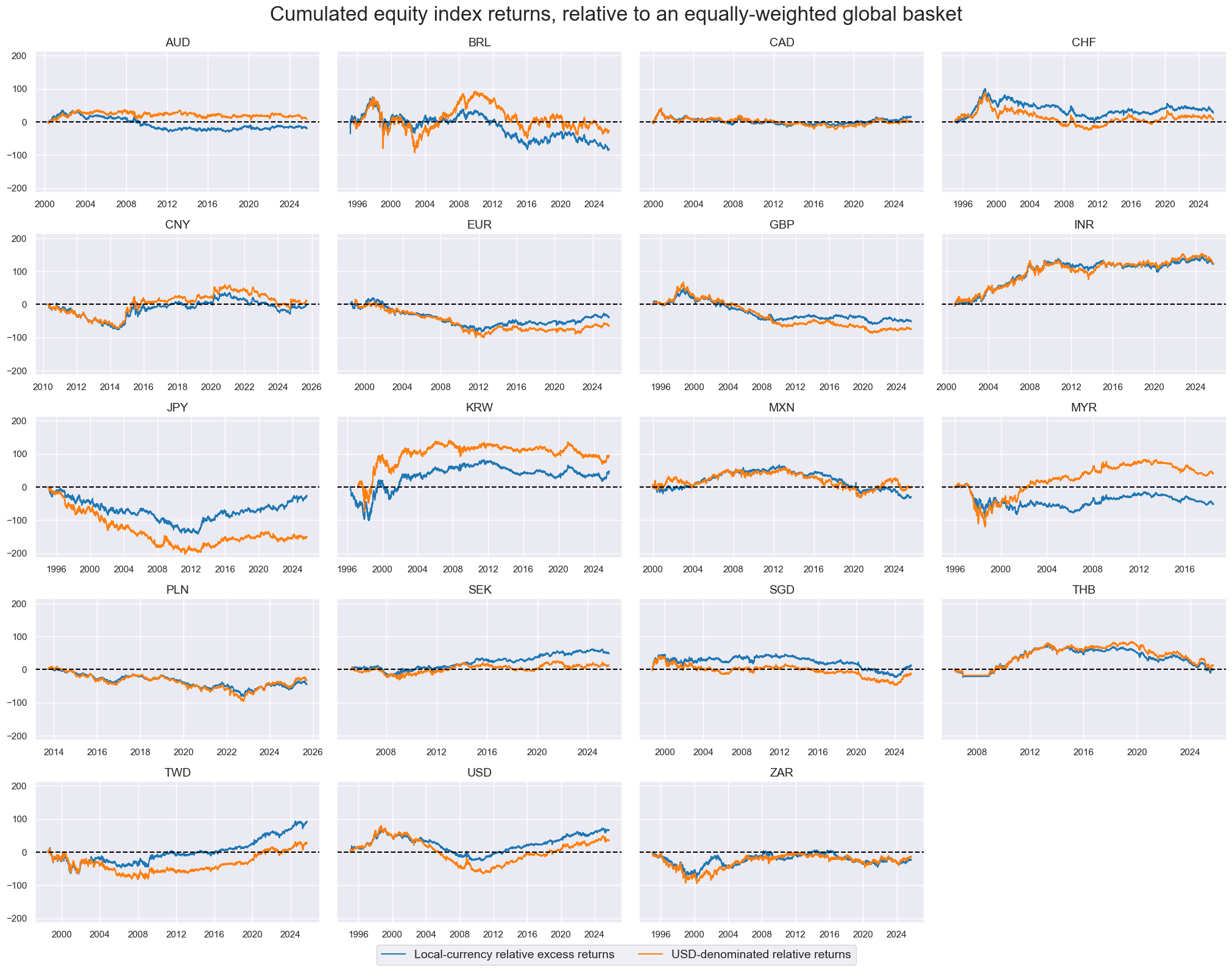
The timeline facet below shows cumulative relative equity index excess returns in both local-currency and U.S. dollar terms, starting in 1995 or from each index’s inception. Here, “relative” means the country index return minus the return of an equally weighted basket of all concurrently tradable countries among the 19 listed above. Because returns are calculated on constant capital, they are symmetric and can accumulate beyond negative 100%.

Relative performance across equity markets can be substantial, often reaching ±50%. For many countries, medium-term local-currency and dollar returns are similar, as both reflect underlying macroeconomic performance. However, long-term outcomes and shorter-term dynamics can differ markedly. For example, Brazil and South Africa have seen much weaker dollar-based results than local-currency returns, while Switzerland and Australia have experienced the opposite. In the short run, equity market declines in emerging markets during crises have been far steeper in dollar terms, highlighting that flexible exchange rates can cushion local equity markets.

Macro factor candidates

In this post, we first pre-select macro factor candidates based on theoretical reasoning. We then choose among them and assign weights using sequential machine learning. This two-stage approach helps avoid data mining and limits hindsight bias. The resulting signals provide a sound basis for statistical tests of predictive power and for strategy backtests.

For the pre-selection of factor candidates, we focus on macroeconomic developments that, in accordance with prevailing macroeconomic theory or common sense, cause differences between the USD returns across countries. For trading, we rely on point-in-time quantitative-fundamental (or “quantamental”) information of such developments in conjunction with the assumption of rational inattention (view post here) of the market. Inattention implies that not all economic information is priced immediately and efficiently.

Analytically, dollar-denominated exposure to foreign equity markets can be separated into two components: foreign exchange exposure and local-currency equity exposure. The selection of macro trading factors should address both dimensions. Broadly, economic developments fall into two categories:

• Unequivocal effects: These either push local equity and FX returns in the same direction or affect only one component while leaving the other neutral.
• Ambiguous effects: These push local equity and FX returns in opposite directions. Without additional analysis or information, the net impact cannot be determined, making the factor’s predictive stability uncertain. Fortunately, there are methods to resolve such ambiguities.

Point-in-time information on relevant economic developments can be expressed as conceptual macro (quantamental) factors. These can be built using macro-quantamental indicators from the J.P. Morgan Macrosynergy Quantamental System (JPMaQS). In practice, low-level indicators are often combined into broader, more abstract economic themes. The construction method depends on whether the factors capture unequivocal effects or ambiguous effects.

In the case of unequivocal effects, we first select a representative set of similar macro-quantamental indicators across all countries (also called “quantamental categories”). The search and browsing for appropriate categories can start from the “Themes” page of the online macro-quantamental academy. Then, we normalize each category around its neutral level sequentially and based on the full data panel (i.e., the dataset of time series for all countries) up to each point in time of the information history. Finally, we average all normalized indicator scores and re-normalize that average sequentially to get the conceptual macro factor score. We also set the sign of the score such that its theoretical impact is always positive for equity returns. For details, see the accompanying Jupyter notebook.

In this post, we have calculated six conceptual macro factors that represent unequivocal economic developments with respect to USD equity returns:

• External balances measure the difference between exports and imports as a ratio to GDP. External balance strength often testifies to the competitiveness of the local economy and, if the central bank is leaning against appreciation through unsterilized intervention, bodes well for local liquidity supply. As constituent quantamental categories, we use the 1-year moving average of the current account balance as % of GDP (documentation), the 1-year moving average of the merchandise trade balance as % of GDP (documentation), and 3-month seasonally-adjusted trade and current account balances as % of GDP minus the 5-year moving average (documentation here and here).
• Currency weakness measures the negative, inflation-adjusted deviation of a currency’s current value from historical or theoretical benchmarks. A weaker currency boosts future earnings growth in local-currency terms for companies with foreign sales and subsidiaries. This factor draws on two quantamental categories: shifts toward undervaluation relative to purchasing power parity, and openness-adjusted real depreciation. The former is represented by the negative trend of the ratio of the PPP exchange rate to the current market FX spot rate as a percentage of the latest month over the previous year (documentation). Real openness-adjusted depreciation is measured as a percentage of the latest week compared to the previous four weeks (documentation), as a percentage of the latest month compared to the same month a year ago, and as a percentage of the latest month compared to the previous 12 months (documentation).
• Terms-of-trade improvement captures short- and medium-term changes in the ratio of exports and import prices. Rising terms of trade support competitiveness, domestic income generation, and currency strength. Dynamics are measured as % of the latest month over a year ago, % of the latest month over the previous 1-year average, and % of the latest week over the previous four weeks (documentation).
• Investment positions improvements show medium-term trends in cross-border investment positions. Improving net investment positions or diminishing liabilities support local funding conditions and limit vulnerability to sudden financial flow stops or reversals. The conceptual factor is calculated based on two dynamics: the change (over a year ago) of net international investment position as % of GDP (documentation), and the negative change of international liabilities as % of GDP  (documentation).
• Liquidity growth focuses on recent trends in estimated central bank (base) money injections in the economy associated with FX interventions or security purchases. Liquidity growth supports local equity markets directly and, if it is combined with FX interventions, also hints at deferred currency appreciation pressure. The underlying quantamental indicators of the factor are 3-month and 6-month changes in intervention liquidity as a ratio to GDP (documentation).
• Economic confidence improvement captures positive economic momentum via both local manufacturing and consumer sentiment improvements, which should be supportive for both local-currency equity and FX returns. The underlying quantamental indicators are manufacturing business confidence difference of the last 3 months over the previous 3 months and the difference over a year ago (documentation), as well as consumer confidence differences of the same type (documentation).

For economic developments with ambiguous effects, we also select representative categories. However, to balance opposing effects on local currency equity and FX returns, we apply what we call the “Costa method” of disambiguation. First, we provide not only absolute indicator levels but also relative ones that are better measures of the FX effects. Then we combine the absolute and relative quantamental indicator levels according to the following formula:

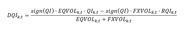
where

QI_k,t is the quantamental indicator value of country k at time t,
RQI_k,t is the relative quantamental indicator value of country k at time t,
DQI_k,t is the disambiguated quantamental indicator value of country k at time t,
sign(QI) is the sign of the theoretical impact of the quantamental indicator on the local equity index future returns,
EQVOL_k,t is the realized annualized standard deviation of local-currency equity index futures returns in country k at time t based on an exponential moving average of daily returns with a half-life of 11 active trading days (documentation), and
EQVOL_k,t is the realized annualized standard deviation of FX forwards returns versus the U.S. dollar for the currency of country k at time t based on an exponential moving average of daily returns with a half-life of 11 active trading days (documentation).

This formula implies that the impact of an ambiguous economic development on USD equity returns depends on the relative volatility of equity index and FX forward returns, as well as on the size of absolute versus relative indicator values. For instance, if an indicator is theoretically positive for equities and equity volatility is much higher than FX volatility, the absolute effect will dominate. If FX volatility is higher and relative indicator values are larger, the relative effect will dominate instead. In both cases, the transformation requires no estimation and produces a presumed positive predictor of USD equity returns. The resulting disambiguated indicators are then normalized, combined, and re-normalized in the same way as those for unequivocal developments.

• The excess inflation effect uses the differences between various headline and core CPI inflation and the effective local inflation targets, all scaled by the local effective inflation target. Higher excess inflation calls for tighter monetary policy and, hence, is negative for local equity returns but positive for FX returns. The underlying quantamental categories are annual headline and core inflation (documentation here and here), and short-term, 3 months over 3 months, seasonally and jump-adjusted headline and core CPI trends (documentation here and here).
• The overheating effect collects evidence of the economy being overstimulated and growing above its productive capacity. Overheating bodes for monetary tightening and, hence, is also a headwind for local equity returns but supportive of currency returns. The quantamental categories used for its calculation are related to domestic demand and the labor market. On the demand side, they include annual real consumption growth (documentation) and annual real retail sales growth (documentation) relative to a 5-year mean of real GDP growth (documentation). On the labor market side, the underlying quantamental indicators are the annual change in unemployment rate (documentation) and the latest unemployment rate vs the trailing five-year average  (documentation).
• The real rates effect summarizes the effects of level and recent changes in real interest rates. High or rising real interest rates bode ill for equity futures returns, but, in relative terms, they are supportive of the local currency FX forward returns. Real interest rate factors are calculated based on the local money market rates (documentation), as well as 2-year and 5-year real IRS interest rates (documentation). We examine the level and change of the latest month (21 days) compared to the previous month.

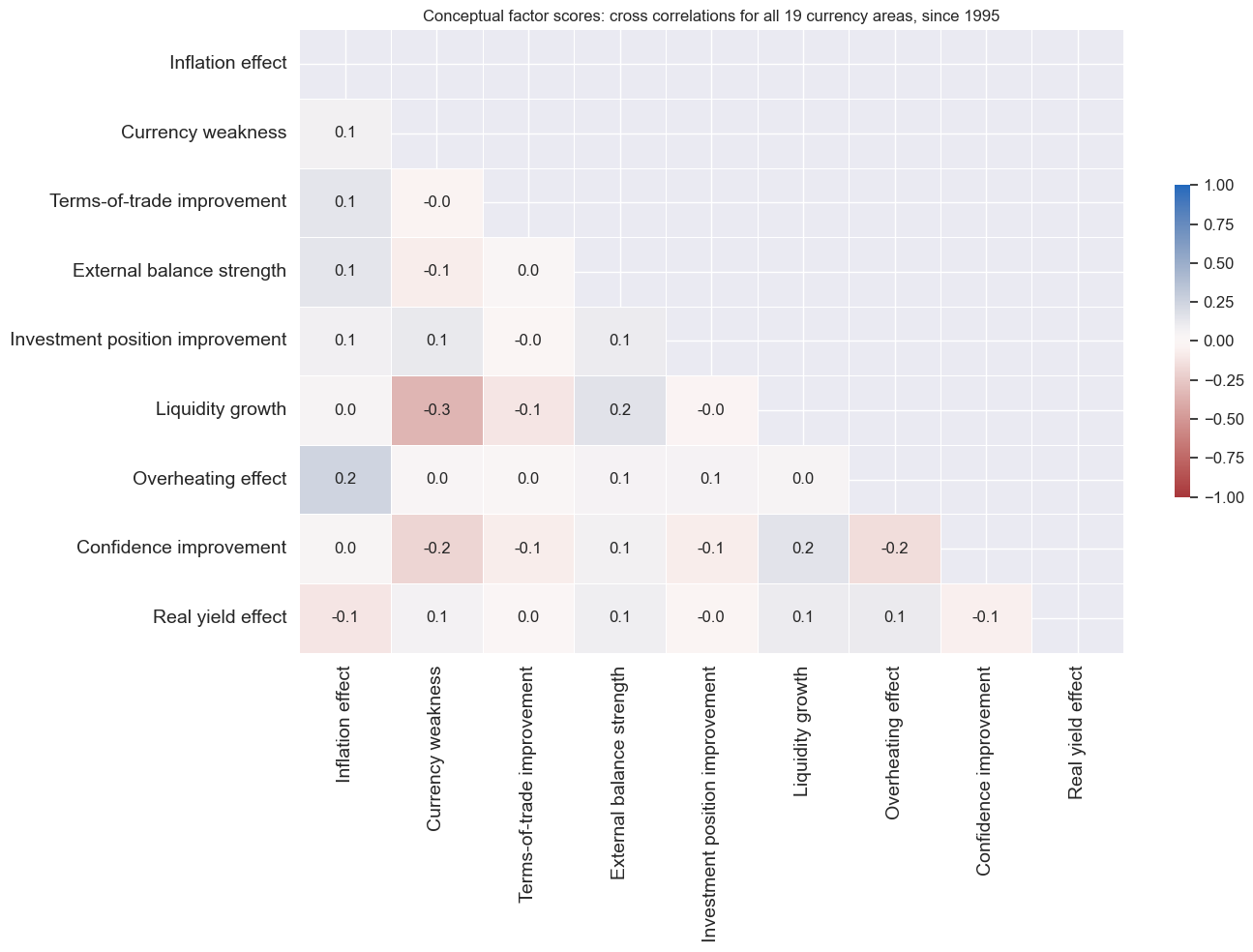
Linear correlation across the nine conceptual factors since 1995 has been diverse and, on average, quite modest based on monthly averages. Only one in 36 concurrent cross-correlations reached 30% and it was a negative relation between currency weakness and liquidity growth.

A sequential machine learning approach to signal construction

To assess the added value of cross-country equity allocation with macro factors, we first evaluate the predictive power and economic value of relative conceptual factors. Relative factors here are differences between the factor scores calculated above and an average of all scores that are available and tradable at a given point in time. The targets for this analysis are relative volatility-targeted USD returns of the 19 countries. This means that conceptually, we only want to predict cross-country returns, not directional global equity returns.

Predictive signals are combinations of the above nine factors in relative form. There is little theory to guide this combination, and it is essential that we avoid hindsight in selection and weighting. Hence, we deploy a sequential machine learning method that was explained in previous posts (e.g., “Macro trading signal optimization: basic statistical learning methods“).

• We first define models and hyperparameters that could explain the relation between factors and target returns. Here, we consider two types of model grids, one for unregularized regressions and one for regularized regressions of the Ridge type. The unregularized regression grid offers non-negative least squares and time-weighted non-negative least squares to the learning process, with or without intercept, and, for the time weights, exponential moving averages with half-lives between one and five years. “Non-negative” here means that the models do not allow coefficients that are at odds with the theoretical direction of the prediction. The Ridge regression grid also offers models with and without intercept, but its main parameter is the penalty coefficient that determines the strength of regularization.
• We begin by defining models and hyperparameters that could capture the relationship between factors and target returns. Two model grids are considered: one for unregularized regressions and one for Ridge (regularized) regressions. The unregularized regression grid includes non-negative least squares and time-weighted non-negative least squares, with or without an intercept. Time weighting uses exponential moving averages with half-lives from one to five years. “Non-negative” means coefficients cannot take signs opposite to the theoretical prediction. The regularized regression grid includes Ridge non-negative least squares regression models with and without an intercept, with the key hyperparameter being the penalty coefficient controlling the strength of regularization.
• Then we set the rules for cross-validation, i.e., the assessments of how well different models perform in predicting unseen data. To this end, we determine the splitters for the sequentially expanding data panels that divide at each point in time the observed periods of time into training and validation sets. Here we do so by using the ExpandingKFoldPanelSplit class of the Macrosynergy package, which is a panel data analogue to the TimeSeriesSplit splitter of scikit-learn. We must also set the optimization criterion for cross-validation, which here is the negative mean squared error of predictions.
• Finally, we perform the actual sequential optimizationwith the Macrosynergy package’s specialized Python class (SignalOptimizer). It applies scikit-learn cross-validation to the specific format of macro-quantamental panel data. Here, it uses data from 2000 to start selecting optimal models and calculating optimized signals based on the nine factors from 2003. Although many quantamental categories date back to the 1990s, scikit-learn is limited to operating on full data sets, which means the shortest factors (inflation effects and real yield effects) restrict the learning history’s score.

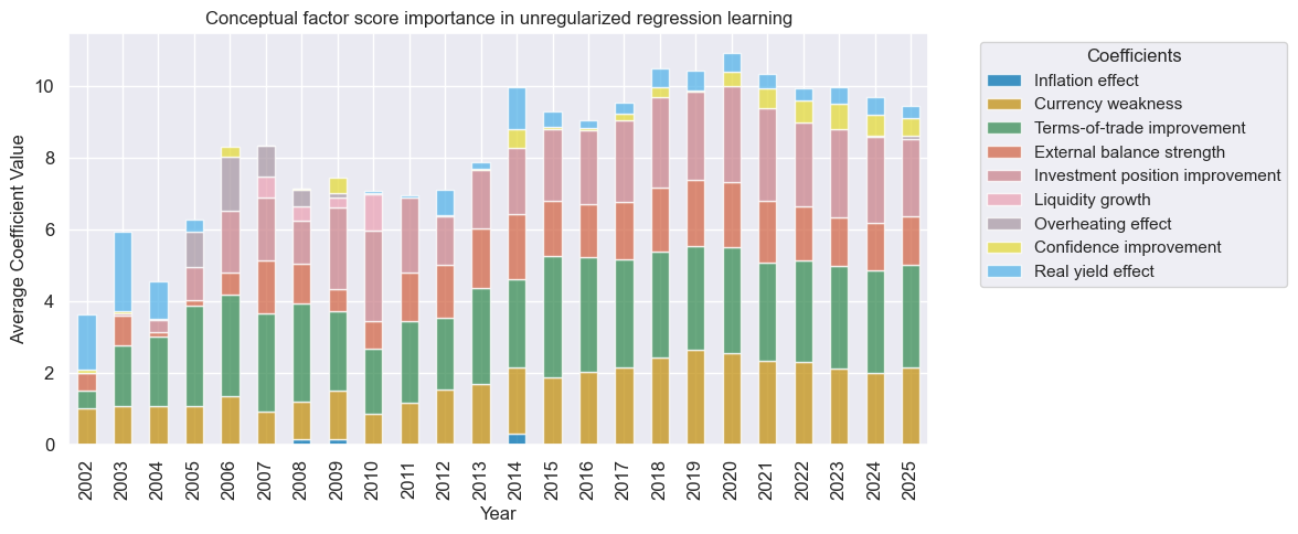
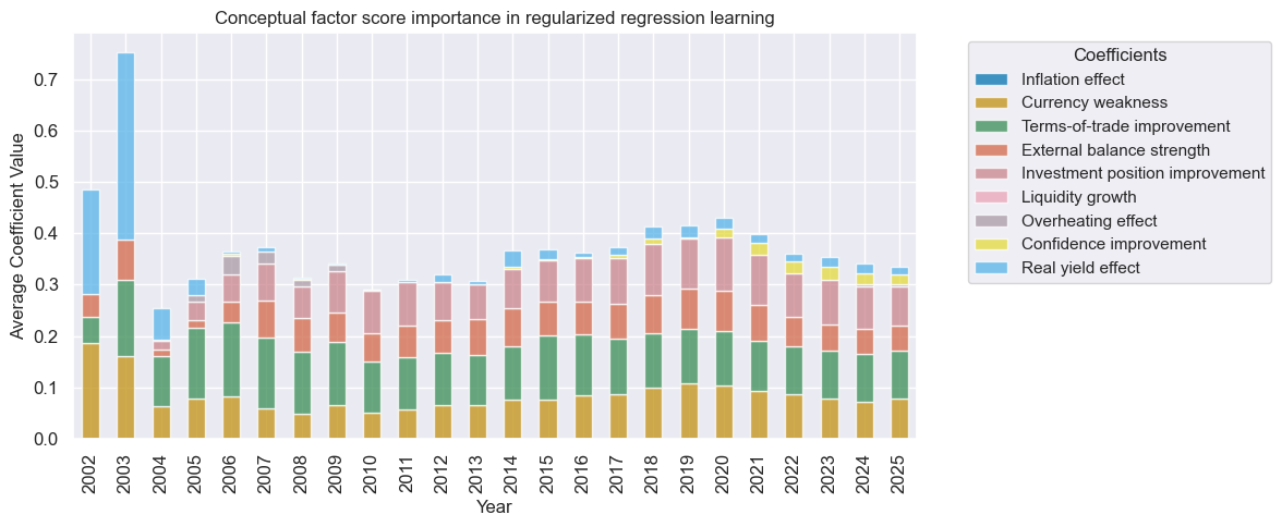
The charts below show the coefficients of normalized conceptual factor scores in optimal models as annual averages over time, as an indication of the relative importance of the candidate concepts. The unregularized and regularized regression methods converged on similar preferences as the sample size increased. The largest weights were ultimately given to terms-of-trade improvements, currency weakness, and improvements in the international investment positions. Notable weights were also assigned to external balances strength, real rates effects, and economic confidence improvement. Thus, five out of the six dominant factors were unequivocal effects.

Dollar-based cross-country equity trading

To analyze the predictive power and economic value of relative cross-currency equity signals, we use the signals generated by sequential learning, which are largely free of hindsight, for forecasting relative returns and trading relative positions. Relative here means USD equity positions in one country versus an equally vol-weighted basket of all tradable countries.

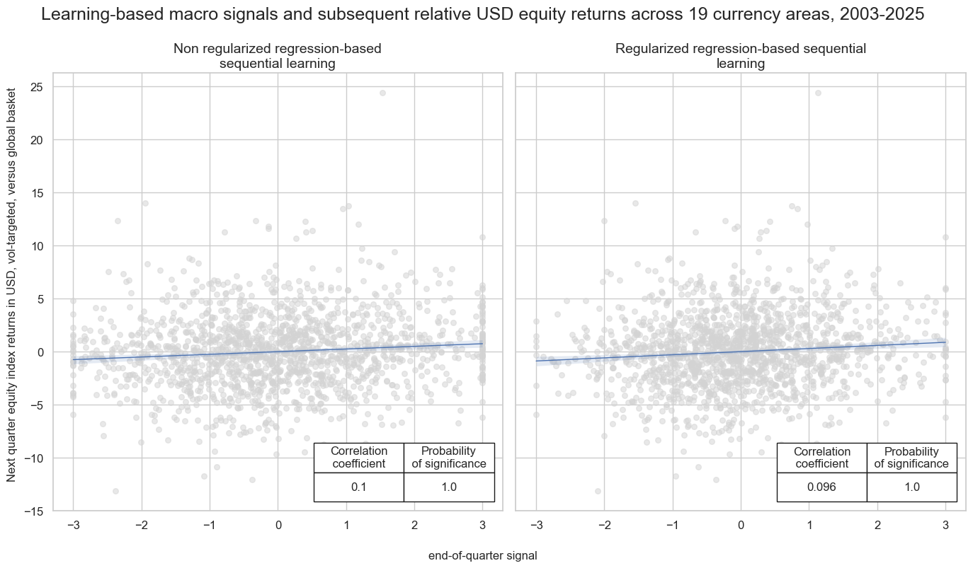
Leaning-based signals have been highly significant positive predictors of cross-country and intertemporal relative return variations both at a monthly and quarterly frequency since 2004. According to the Macrosynergy panel test, the probability that the relations are significant and not accidental is near 100%, and equally strong for non-regularized and regularized regression-based learning.

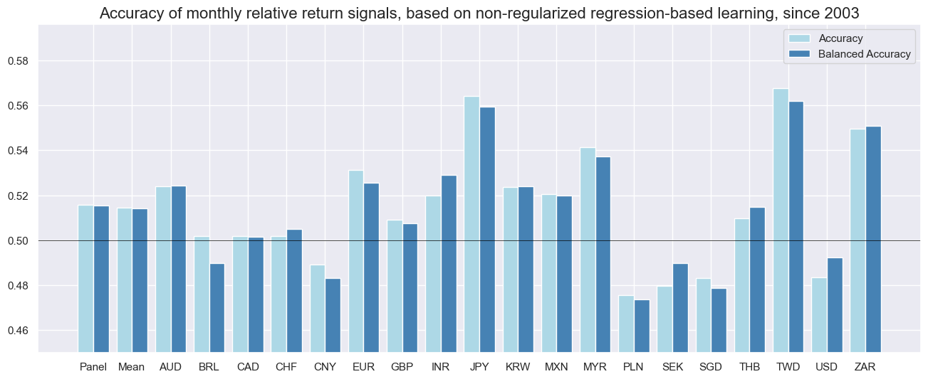
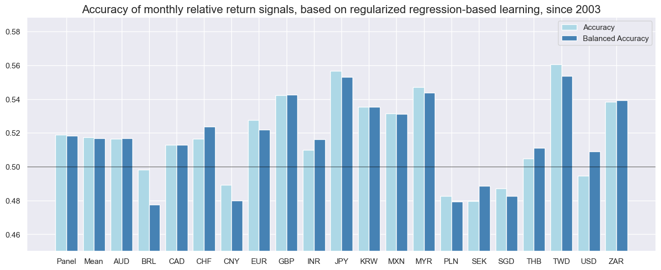
Monthly prediction accuracy has generally been well above 50%, though it varies widely across countries. For the overall panel, both simple accuracy (share of correctly predicted return signs) and balanced accuracy (average accuracy for positive and negative returns) have been about 52%. China, Poland, Singapore, and the U.S. scored below 50% for both learning signal types, while the UK and Switzerland also fell below 50% for non-regularized regression signals. The other 13 countries achieved accuracy above 50%. The differences in accuracy suggest that our simplistic macro factors may not be sufficiently customized to structural differences across countries. One way to mend this is the “global-local” method of machine learning for generating international macro trading signals (view post here).

The strong positive correlation and high accuracy of the combined macro signals should generate economic value when applied to basic trading rules. We test this using a naïve PnL approach: month-end signals from the learning process determine positions for the start of the next month, with a one-day gap for execution. Signal size is capped at three standard deviations as basic risk control. The PnLs ignore transaction costs and compounding, and are scaled to a 10% annualized volatility for easier return comparison.

Both types of learning signals have produced 22-year Sharpe ratios of approximately 0.7 and Sortino ratios of 1-1.1 with negative correlation to S&P500 returns. This suggests that these relative returns were additive, without requiring additional outright long equity exposure. There has also been no correlation to U.S. fixed income returns. There has been seasonality, i.e., time variation in returns, but it was modest by the standards of macro trading strategies. The best 5% of monthly performance contributed a bit more than half to the long-term PnL. Overall, the naïve PnL has displayed a persistent and significant upward trend for over two decades.

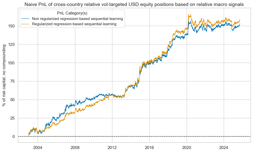
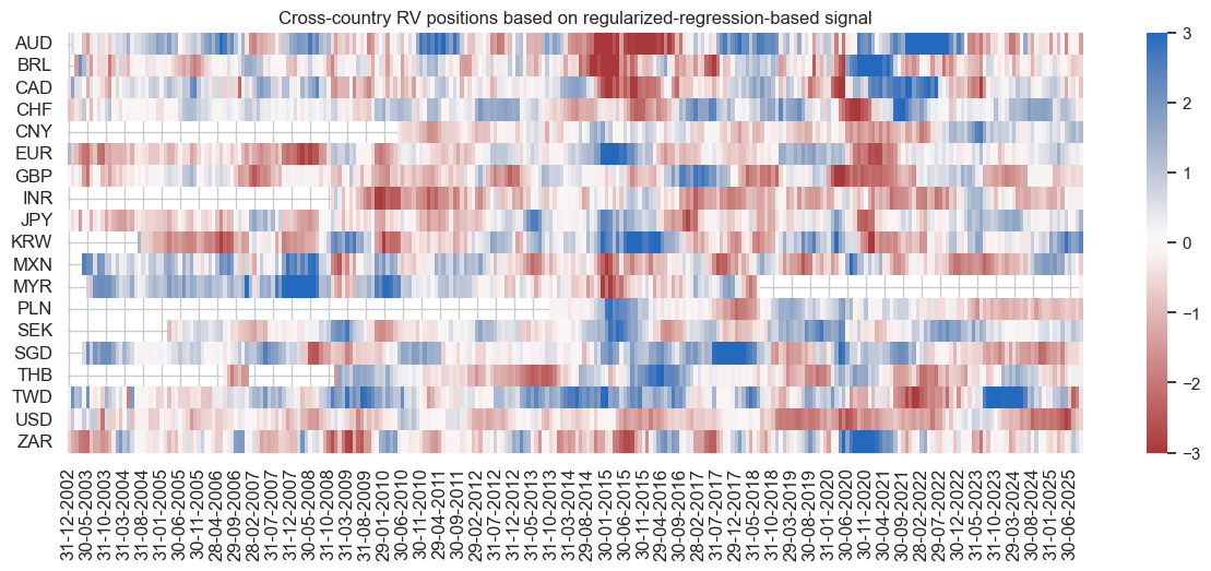
Transaction costs can eat into these added returns, particularly if positions are taken in large sizes and rebalanced in short time periods. However, long and short positions have historically been highly autocorrelated, often lasting for multiple years, as illustrated in the positioning heatmap below.

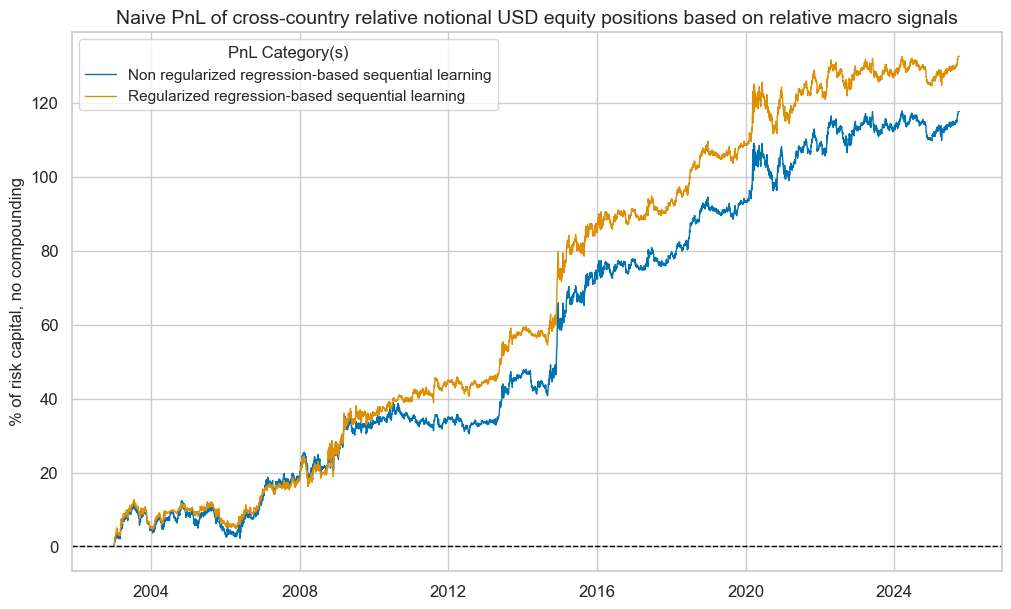
Applying the relative signals to relative notional (non-vol-targeted) positions would still have delivered substantial long-term returns, with Sharpe ratios around 0.6 and negative equity correlations. Seasonality was slightly higher, largely because the machine learning signals struggled in their early years with only short historical samples. Overall, the results further support the use of cross-country trading signals as a solid foundation for setting cash portfolio allocation weights.

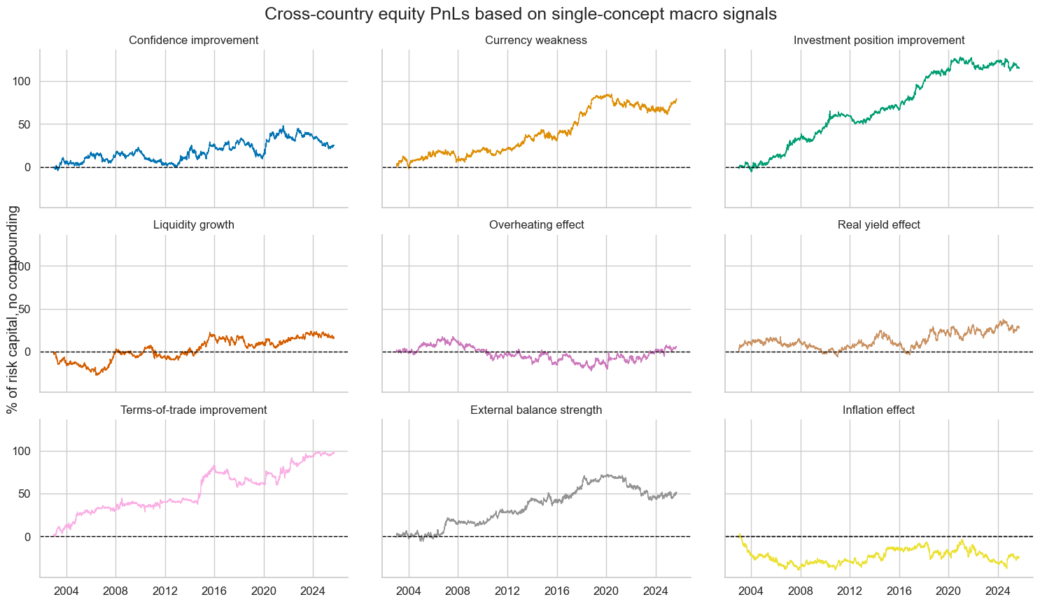
The timeline facet below shows naïve PnLs based on single conceptual factor scores. With hindsight, the strongest PnL generators have been the international investment position improvements, terms-of-trade improvements, currency weakness, and external balance strength.

A rules-based enhancement of real money portfolios

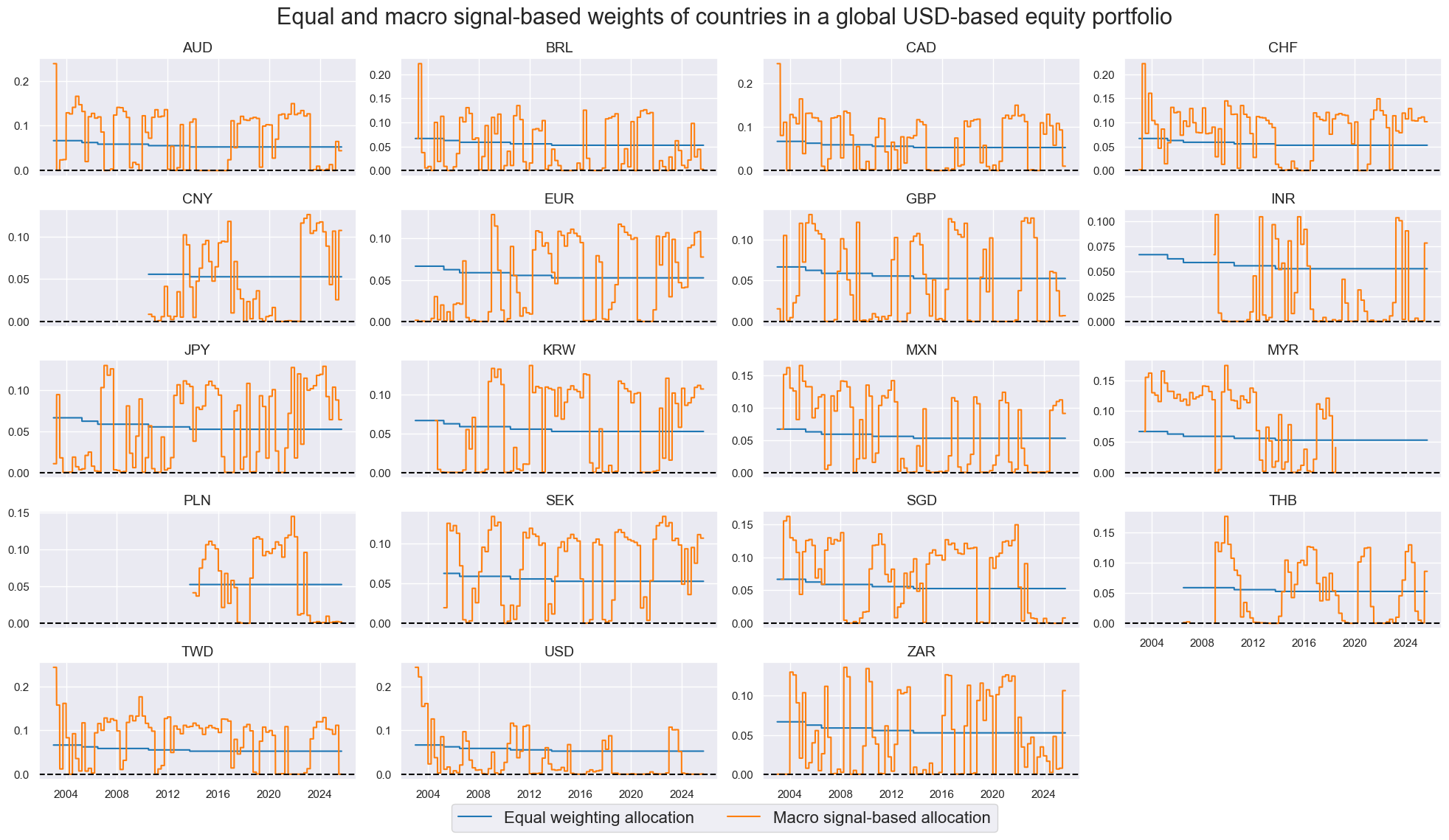
This final section demonstrates the value of using macro factors for cross-country allocation in the equity portfolio of a dollar-based investor. We use the learning-based relative signals to determine the weights of a 19-country portfolio, modifying default equal weights according to a quarterly portfolio rebalancing rule. We chose a quarterly frequency for this proof of concept to keep transaction costs low.

For consistency, we adapt country weights to macro signals using the same method as in an earlier post on sovereign bonds. We multiply the original equal weights by a sigmoid (logistic) function of the relative signal scores, then rescale the weights to sum to one. The sigmoid is set so weights range from zero (for very negative signals) to about twice the original equal weight (for very positive signals), though rescaling can sometimes make them slightly higher.

The timeline facet below shows modified and equal weights based on the regularized regression-based signals. Changes can be sizable, up to 20% of the overall portfolio value, but are rare, about once per year and country. Also, with a quarterly rebalancing frequency, a high-volume strategy can rebalance very gradually.

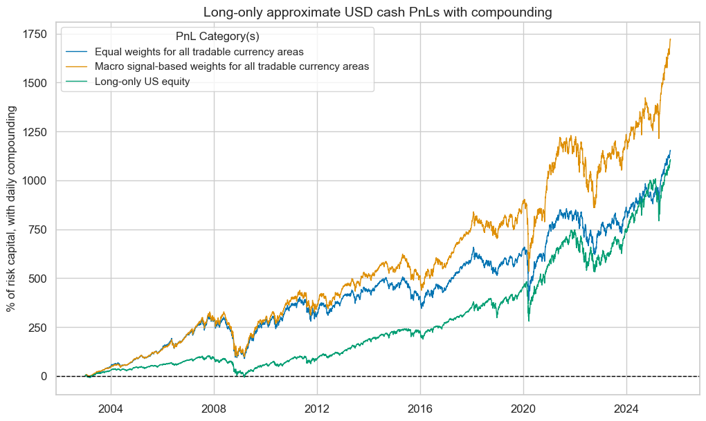
Then we simulate naïve PnLs for a dollar-based portfolio that allocates funds to either the U.S. market (broad all-caps basket of 2250 stocks), an equally weighted international book, and a macro-weighted international book. Over the past 22 years, the portfolio with the macro-based weights has outperformed in both risk-adjusted and percent returns. The annual return of the macro-signal-based portfolio has been nearly 14%, versus 12.6% for the international portfolio and 12.2% for the U.S. portfolio, prior to transaction costs. Due to the compounding of excess returns, the macro-weights would have ultimately produced roughly one-and-a-half times the USD cash returns of the reference books, which over 22 years added up to about 5 times the originally invested capital.

Annex 1: Equity indices

This post looks at eight developed market local-currency index futures and eleven emerging market local-currency index futures. The developed market indices are (in alphabetical order of currency symbol):

• AUD: The S&P/ASX 200 is the primary index for the Australian equity market. It measures the performance of the 200 largest companies by market capitalization listed on the Australian Stock Exchange (ASX).
• CAD: The S&P/TSX 60 Index is designed to represent the large-cap segment of the Canadian equity market. It includes 60 of the largest and most liquid companies listed on the Toronto Stock Exchange (TSX).
• CHF: The Swiss Market Index (SMI) is Switzerland’s premier stock market index, representing the 20 largest and most liquid companies listed on the SIX Swiss Exchange.
• EUR: The EURO STOXX 50 Index is a leading stock market index for the euro area, representing the 50 largest and most liquid blue-chip companies from 11 Eurozone countries.
• GBP: The FTSE 100 Index is a stock market index representing the 100 largest publicly listed companies by market capitalization on the London Stock Exchange (LSE).
• JPY: The Nikkei 225 Stock Average Index is a prominent stock market index in Japan, representing 225 of the largest and most liquid companies listed on the Tokyo Stock Exchange (TSE).
• SEK: The OMX Stockholm 30 (OMXS30) Index is a major stock market index in Sweden, representing the 30 most traded large-cap companies listed on the Nasdaq Stockholm exchange.
• USD: The S&P 500 Composite Index is one of the most widely followed stock market indices in the world, representing 500 of the largest publicly traded companies in the United States. (Note that even though the U.S. is about twice the size of the euro area, the market capitalization of the S&P500 has been roughly ten times that of EURO STOXX.)

The emerging market indices are:

• BRL: The Brazil Bovespa Index, also known as the Ibovespa is the main stock market index in Brazil, representing the performance of the most actively traded companies on the B3, the São Paulo Stock Exchange.
• CNY: The Shanghai Shenzhen CSI 300 index is a benchmark in China that tracks the 300 largest and most liquid A-share stocks traded on the Shanghai Stock Exchange (SSE) and the Shenzhen Stock Exchange (SZSE).
• INR: The CNX Nifty (50) is the flagship stock market index of the National Stock Exchange of India. It represents the weighted average of 50 of the largest and most actively traded stocks spanning 13 sectors of the Indian economy.
• KRW: The KOSPI 200 Index is a major stock market index in South Korea, representing the performance of the 200 largest and most liquid companies listed on the Korea Exchange (KRX).
• MXN: The Mexico IPC, often referred to as the Bolsa Index, is the main stock market index in Mexico. It tracks the performance of the 35 largest and most liquid companies listed on the Mexican Stock Exchange.
• MYR: The FTSE Bursa Malaysia KLCI (Kuala Lumpur Composite Index) is the main stock market index in Malaysia. It tracks the performance of the 30 largest companies by market capitalization listed on the Bursa Malaysia
• PLN: The Warsaw General Index 20 comprises the 20 largest and most liquid companies listed on the Warsaw Stock Exchange (WSE) in Poland.
• SGD: The MSCI Singapore (Free) Index represents the performance of the Singapore equity market through a free float-adjusted market capitalization-weighted index.
• THB: The Bangkok SET 50 Index is a major stock market index in Thailand, representing the 50 largest companies listed on the Stock Exchange of Thailand.
• TWD: The Taiwan Stock Exchange Weighted Index (TAIEX) is the main stock market index in Taiwan. It tracks the performance of all listed companies on the Taiwan Stock Exchange.
• TRY: The BIST 30 Index is one of the leading stock market indices of Turkey, tracking the 30 largest and most liquid companies listed on Borsa Istanbul.
• ZAR: The FTSE/JSE Top 40 Index is a key stock market index in South Africa, representing the 40 largest companies listed on the Johannesburg Stock Exchange (JSE) by market capitalization.