External balance ratios #
This category group contains key real-time measures of external balances of trade and finance, as a percentage of concurrent nominal GDP. These balances are typically viewed as 1-year trailing moving averages or as shorter-term seasonally-adjusted averages.
External balance ratios serve as indicators of demand for the local currency and vulnerability to international financial market shocks.
Current account-to-GDP ratio #
Ticker : CABGDPRATIO_NSA_12MMA / CABGDPRATIO_NSA_1YMA / CABGDPRATIOE_NSA_12MMA
Label : External current account as % of GDP: 12-month moving average / latest published year / 12-month moving average, enhanced.
Definition : External current account balance as % of nominal GDP, latest month(s) predicted by customs trade balance: 12-month moving average / latest published year / 12-month moving average, enhanced by other stable flows.
Notes :
-
The current account balance comprises external goods and services trade balances, net factor income, and net transfer payments (such as foreign aid).
-
A positive balance means a positive net demand for the domestic currency related to these transactions.
-
Often external goods trade balances are published before overall balance of payments. In these cases, JPMaQS estimates current account balances based on the latest customs merchandise trade balances. In particular, the latest monthly current balance is estimated as the balance a year ago plus the difference of the merchandise trade balance compared to a year ago.
-
These tickers are available for frontier markets.
-
The enhanced indicator builds on the concept of the external current accounts by incorporating two additional sources of stable external flows: sovereign wealth fund outflows and stable net errors and omissions.
-
We estimate sovereign wealth fund outflows and subtract these from the current account balance, as they typically represent a sustained flow. This adjustment currently only applies to SGD and NOK. To estimate sovereign wealth fund outflows, we rely on balance of payments data. For Norway, we aggregate all general government items under the “Portfolio Investments” and “other investments” categories. These estimates closely align with the outflows reported in the Norwegian SWF’s annual reports. For Singapore, we follow a similar approach, combining all “official” items within the same categories. However, unlike Norway, Singapore’s primary sovereign wealth fund does not disclose outflow data for direct comparison.
-
The net errors and omissions component of the Balance of Payments may contain hidden stable flows, such as unregistered imports (also known as “suitcase trade” or “shuttle trade”). Since legitimate errors and omissions should theoretically be equally likely to be positive or negative, we detect errors that are consistently positive or negative as an indication of stable flows. These identified flows are then added to the current account balance. See Appendix 4 for further details.
Ticker : CABGDPRATIO_SA / CABGDPRATIO_SA_3MMA
Label : External current account as % of GDP: seasonally adjusted / seasonally adjusted, 3-month moving average.
Definition : External current account balance as % of nominal GDP: seasonally adjusted / seasonally adjusted, 3-month moving average.
Notes :
-
The current account balance comprises external goods and services trade balances, net factor income, and net transfer payments (such as foreign aid).
-
A positive balance means a positive net demand for the domestic currency related to these transactions.
-
Current account balances are published by the national sources as:
-
Quarterly, non-seasonally adjusted: AUD, CAD, CHF, CLP, CNY, COP, INR, IDR, MYR, MXN, NOK, NZD, PEN, RUB, SEK, SGD, TWD, ZAR, ARS, EGP, DOP, PAB, QAR, NGN, SAR, UYU.
-
Monthly, seasonally adjusted: BRL, CZK, EUR, JPY, KRW, PLN, PHP, THB, TRY.
-
Quarterly, seasonally adjusted: HUF, ILS, and USD.
-
Monthly, seasonally adjusted: GBP.
-
-
When JPMaQS does seasonal adjustment for vintages, it adjusts the current account balance ratio to GDP by applying the additive method of the US Census X-13 seasonal adjustment algorithm for each release date, at their native observation frequency (monthly or quarterly). See Appendix 1 for further details.
-
For AUD, CAD, CHF, CLP, COP, INR, IDR, MXN, NOK, NZD, RUB, SEK, and ZAR the national sources series’ have been complemented with additional vintages provided by OECD’s ‘Revision Analysis’ dataset. See also Appendix 2 for details on OECD data integration.
Merchandise trade balance-to-GDP ratio #
Ticker : MTBGDPRATIO_NSA_12MMA
Label : External merchandise trade balance as % of GDP: 12-month average
Definition : External merchandise trade balance as % of nominal GDP: 12-month moving average
Notes :
-
The merchandise trade balance is part of the external balance of payments. It only tracks trade in goods.
-
A positive balance means positive net demand for the domestic currency related to merchandise trade.
-
The indicator use customs trade data for the latest months for countries that publish a customs report before the balance of payments and in good-quality.
-
These tickers are available for frontier markets. We did not include trade balances for AED because oil trade data are not published.
Short-term trade balance-to-GDP ratio #
Ticker : MTBGDPRATIO_SA_3MMA / _6MMA
Label : External merchandise trade balance as % of GDP: 3-month average (sa) / 6-month average (sa)
Definition : External merchandise trade balance as % of nominal GDP: seasonally-adjusted 3-month moving average / 6-month moving average
Notes :
-
The merchandise trade balance is part of the external balance of payments, but only tracks trade in goods.
-
Seasonal adjustment factors are sequentially re-estimated as new data are being released. Every re-estimation gives rise to a new data vintage which is the basis of concurrent trend estimation. See Appendix 1 for further details.
-
For most countries calendar adjustment is applied, accounting for working day effects or moving holidays (e.g. Chinese New Year, Easter, Diwali, Ramadan etc).
Net FDI-to-GDP ratio #
Ticker : NFDIGDPRATIO_NSA_12MMA
Label : Net foreign direct investment as % of GDP.
Definition : Net foreign direct investment as % of nominal GDP, 1-year moving trimmed mean.
Notes :
-
The indicator measures the net inward and outward flow of foreign direct investment of a currency area, with a 1-year lookback horizon and as a % of GDP.
-
All other things equal, a positive balance means positive net demand for the domestic currency related to cross-border direct investment.
-
Due to occasional large transactions, the net FDI balance is prone to outliers. Therefore, instead of conventional 1-year moving averages, JPMaQS uses medians (if original data are quarterly frequency) or 50% trimmed means (if original data are monthly frequency). In both cases the measure is based on the inner 50% of the values in the 1-year lookback window. This delivers a more robust assessment of the underlying trends in direct investment flows.
Basic external balance-to-GDP ratio #
Ticker : BXBGDPRATIO_NSA_12MMA / BXBGDPRATIOE_NSA_12MMA
Label : External basic balance as % of GDP: 12-month moving average / 12-month moving average, enhanced.
Definition : External basic balance as % of nominal GDP, latest month(s) predicted by customs trade balance: 12-month moving average / 12-month moving average, enhanced by other stable flows.
Notes :
-
This indicator is one of the broadest representations of stable external flows, taking into account both investment and trade flows into the currency area. A positive balance means positive related net demand for the domestic currency.
-
In order to avoid large distortions in the net FDI balance we use a 50% trimmed mean over the past year, rather than a simple moving average.
-
The enhanced indicator builds on the concept of the external current accounts by incorporating two additional sources of stable external flows: sovereign wealth fund outflows and stable net errors and omissions.
-
We estimate sovereign wealth fund outflows and subtract these from the current account balance, as they typically represent a sustained flow. This adjustment currently only applies to SGD and NOK. To estimate sovereign wealth fund outflows, we rely on balance of payments data. For Norway, we aggregate all general government items under the “Portfolio Investments” and “other investments” categories. These estimates closely align with the outflows reported in the Norwegian SWF’s annual reports. For Singapore, we follow a similar approach, combining all “official” items within the same categories. However, unlike Norway, Singapore’s primary sovereign wealth fund does not disclose outflow data for direct comparison.
-
The net errors and omissions component of the Balance of Payments may contain hidden stable flows, such as unregistered imports (also known as “suitcase trade” or “shuttle trade”). Since legitimate errors and omissions should theoretically be equally likely to be positive or negative, we detect errors that are consistently positive or negative as an indication of stable flows. These identified flows are then added to the basic external balance. See Appendix 4 for further details.
Net foreign portfolio investment-to-GDP ratio #
Ticker : NFPIGDPRATIO_NSA / NFPIGDPRATIO_NSA_2QMA / _4QMA
Label : Net foreign portfolio investment, % of GDP: nsa, nsa, latest quarter / nsa, 2 quarter moving average / nsa, 4 quarter moving average
Definition : Net foreign portfolio investment, % of GDP: non-seasonally adjusted, latest quarter / non-seasonally adjusted, 2-quarter moving average / non-seasonally adjusted, 4-quarter moving average
Notes :
-
Portfolio investment is defined as cross-border transactions and positions involving debt or equity securities, other than those included in direct investment or reserve assets. Equity not in the form of securities (e.g., in unincorporated enterprises) is not included in portfolio investment; it is included in direct or other investment.
-
All other things equal, a positive balance means positive net demand for the domestic currency related to cross-border portfolio investment.
-
The indicator measures the net inward and outward flow of foreign portfolio investment of a currency area over the last quarter as a % of GDP, whereby the GDP is a 4-quarter moving average.
Net foreign lending-to-GDP ratio #
Ticker : NFLGDPRATIO_NSA / NFLGDPRATIO_NSA_2QMA / _4QMA
Label : Net foreign lending, % of GDP: nsa, latest quarter / nsa, 2 quarter moving average / nsa, 4 quarter moving average
Definition : Net foreign lending, % of GDP: non-seasonally adjusted, latest quarter / non-seasonally adjusted, 2-quarter moving average / non-seasonally adjusted, 4-quarter moving average
Notes :
-
The indicator measures the net inward flow of foreign credit of a currency area over the last quarter as a % of GDP, whereby the GDP is a 4-quarter moving average. All other things equal, a positive balance means positive net demand for the domestic currency related to cross-border net lending.
-
Foreign credit is based on two items of the “other investments” category of the balance of payments: trade credit and loans, including credit and loans from the IMF. Generally, other investment is a residual category that includes positions and transactions other than those included in direct investment, portfolio investment, financial derivatives and employee stock options, and reserve assets.
-
SGD only release foreign lending data annually.
Imports #
Only the standard Python data science packages and the specialized
macrosynergy
package are needed.
import os
import numpy as np
import pandas as pd
import matplotlib.pyplot as plt
import seaborn as sns
import math
import json

import macrosynergy.management as msm
import macrosynergy.panel as msp
import macrosynergy.signal as mss
import macrosynergy.pnl as msn


from macrosynergy.download import JPMaQSDownload

from timeit import default_timer as timer
from datetime import timedelta, date, datetime

import warnings

warnings.simplefilter("ignore")
The
JPMaQS
indicators we consider are downloaded using the J.P. Morgan Dataquery API interface within the
macrosynergy
package. This is done by specifying
ticker strings
, formed by appending an indicator category code
<category>
to a currency area code
<cross_section>
. These constitute the main part of a full quantamental indicator ticker, taking the form
DB(JPMAQS,<cross_section>_<category>,<info>)
, where
<info>
denotes the time series of information for the given cross-section and category. The following types of information are available:
-
valuegiving the latest available values for the indicator -
eop_lagreferring to days elapsed since the end of the observation period -
mop_lagreferring to the number of days elapsed since the mean observation period -
gradedenoting a grade of the observation, giving a metric of real time information quality.
After instantiating the
JPMaQSDownload
class within the
macrosynergy.download
module, one can use the
download(tickers,start_date,metrics)
method to easily download the necessary data, where
tickers
is an array of ticker strings,
start_date
is the first collection date to be considered and
metrics
is an array comprising the times series information to be downloaded.
# Cross-sections of interest

cids_dm = [
    "AUD",
    "CAD",
    "CHF",
    "EUR",
    "GBP",
    "JPY",
    "NOK",
    "NZD",
    "SEK",
    "USD",
]  # DM currency areas
cids_dmec = ["DEM", "ESP", "FRF", "ITL", "NLG"]  # DM euro area countries
cids_latm = ["BRL", "COP", "CLP", "MXN", "PEN"]  # Latam countries
cids_emea = ["CZK", "HUF", "ILS", "PLN", "RON", "RUB", "TRY", "ZAR"]  # EMEA countries
cids_emas = [
    "CNY",
    "IDR",
    "INR",
    "KRW",
    "MYR",
    "PHP",
    "SGD",
    "THB",
    "TWD",
]  # EM Asia countries

cids_lc = [  # Latam local currency debt countries
    "BRL", "CLP","COP", "MXN", "PEN", "CZK",
    "HUF", "PLN","RON", "RUB", "TRY",
    "ZAR", "CNY", "IDR", "MYR",
    "PHP", "THB"]


cids_em = cids_latm + cids_emea + cids_emas
cids_frontier = ['ARS', 'AED', 'DOP', 'EGP', 'OMR', 'QAR', 'RSD','SAR', 'NGN', 'PAB','UYU' ]
cids_credit = sorted(list((set(cids_frontier) |  set(cids_lc))) )

cids = sorted(cids_dm + cids_dmec + cids_em + cids_frontier)
cids_fx = sorted(list(set(cids_dm + cids_em) - set(["USD"])))
# Quantamental categories of interest

main = [
    "CABGDPRATIO_NSA_12MMA",
    "CABGDPRATIOE_NSA_12MMA",
    "CABGDPRATIO_NSA_1YMA",
    "CABGDPRATIO_SA",
    "CABGDPRATIO_SA_3MMA",
    "NFDIGDPRATIO_NSA_12MMA",
    "BXBGDPRATIO_NSA_12MMA",
    "BXBGDPRATIOE_NSA_12MMA",
    "MTBGDPRATIO_NSA_12MMA",
    "MTBGDPRATIO_SA_6MMA",
    "MTBGDPRATIO_SA_3MMA",
    "NFPIGDPRATIO_NSA_4QMA",
    "NFLGDPRATIO_NSA_4QMA",
    "NFPIGDPRATIO_NSA_2QMA",
    "NFLGDPRATIO_NSA_2QMA",
    "NFPIGDPRATIO_NSA",
    "NFLGDPRATIO_NSA",
]

econ = ["REER_NSA_P1M60ML1"]  # economic context
mark = [
    "FXCRR_NSA",
    "FXCRR_VT10",
    "FXXR_NSA",
    "FXXR_VT10",
    "DU05YXR_NSA",
    "DU05YXR_VT10",
    "FXXRHvGDRB_NSA",
    "FXTARGETED_NSA",
    "FXUNTRADABLE_NSA",
    "FXXRxEASD_NSA"
    "LCBIR_NSA",
    "LCBIXR_VT10",
    "LCBIXR_NSA",
    "FCBIR_NSA",
    "FCBIXR_NSA",
    "FCBIXR_VT10",
    "CDS05YXR_VT10",
    "CDS02YXR_VT10",
    "GB01YXR_VT10",
    "CDS05YSPRD_NSA",
    "CDS05YXR_NSA"

]  # market links

xcats = main + econ + mark
# Download series from J.P. Morgan DataQuery by tickers

start_date = "1996-01-01"
tickers = [cid + "_" + xcat for cid in cids for xcat in xcats]
print(f"Maximum number of tickers is {len(tickers)}")

# Retrieve credentials

client_id: str = os.getenv("DQ_CLIENT_ID")
client_secret: str = os.getenv("DQ_CLIENT_SECRET")

# Download from DataQuery

with JPMaQSDownload(client_id=client_id, client_secret=client_secret) as downloader:
    start = timer()
    df = downloader.download(
        tickers=tickers,
        start_date=start_date,
        metrics=["value", "eop_lag", "mop_lag", "grading"],
        suppress_warning=True,
        show_progress=True,
    )
    end = timer()

dfd = df

print("Download time from DQ: " + str(timedelta(seconds=end - start)))
Maximum number of tickers is 1824
Downloading data from JPMaQS.
Timestamp UTC:  2025-05-08 15:46:43
Connection successful!
Requesting data: 100%|███████████████████████████████████████████████████████████████| 365/365 [01:25<00:00,  4.28it/s]
Downloading data: 100%|██████████████████████████████████████████████████████████████| 365/365 [00:43<00:00,  8.38it/s]
Some expressions are missing from the downloaded data. Check logger output for complete list.
2704 out of 7296 expressions are missing. To download the catalogue of all available expressions and filter the unavailable expressions, set `get_catalogue=True` in the call to `JPMaQSDownload.download()`.
Download time from DQ: 0:02:26.494341
Availability #
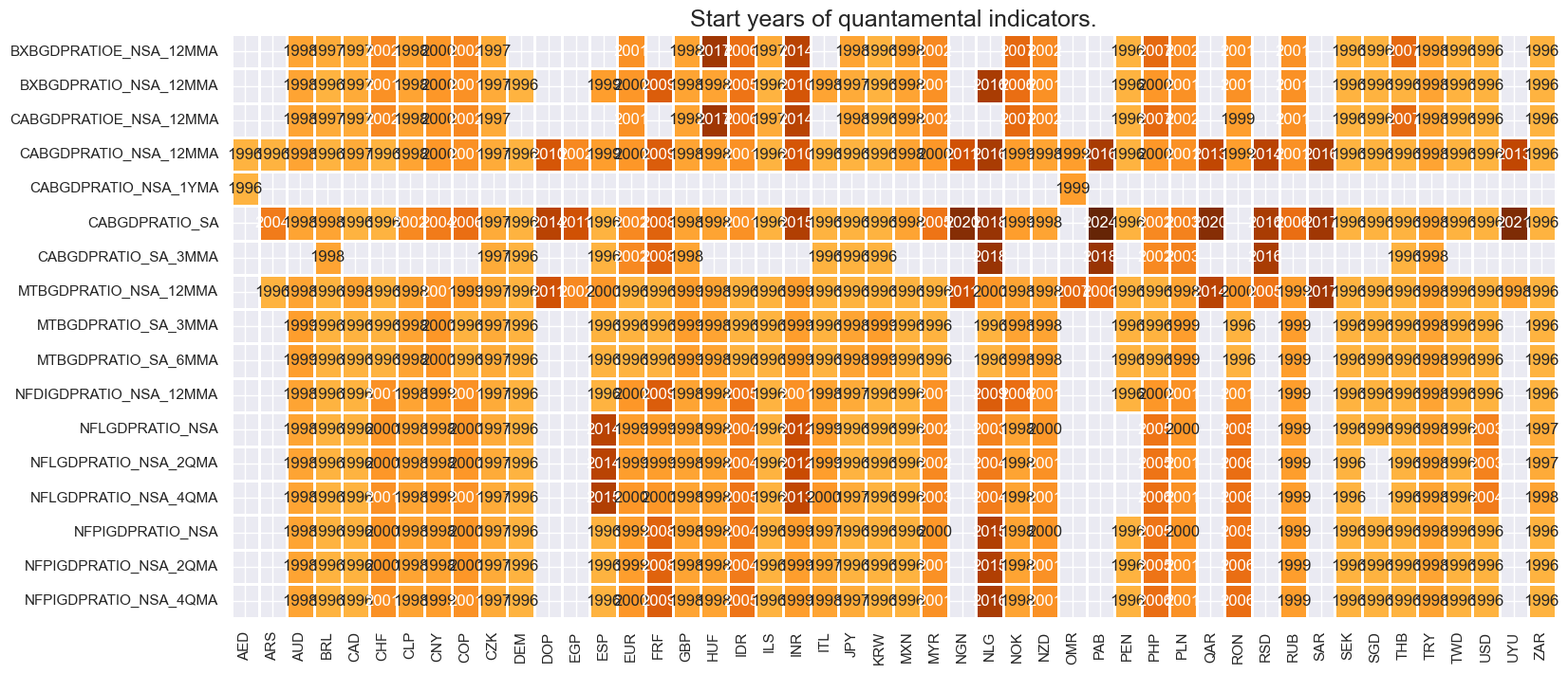
Real-time quantamental indicators of external balance ratios are available from the late 1990s for most cross-sections. Some emerging and most frontier market indicators have shorter history, however.
xcatx =  main
cidx = cids

dfx = msm.reduce_df(dfd, xcats=xcatx, cids=cidx)
dfs = msm.check_startyears(
    dfx,
)
msm.visual_paneldates(dfs, size=(18, 8))

print("Last updated:", date.today())
Last updated: 2025-05-08
For most countries, only recent years’ full set of external balances are pure vintages based only on unrevised data.
cidx = cids
xcatx = main

plot = msp.heatmap_grades(
    dfd,
    xcats=xcatx,
    cids=cidx,
    size=(20, 6),
    title=f"Average external balance ratio vintage grades from {start_date} onwards",
)

History #
External current account ratios #
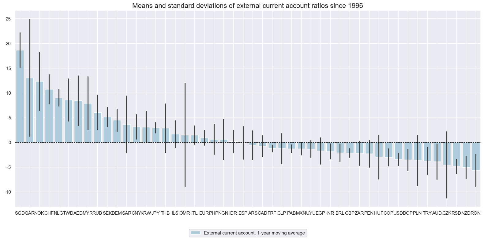
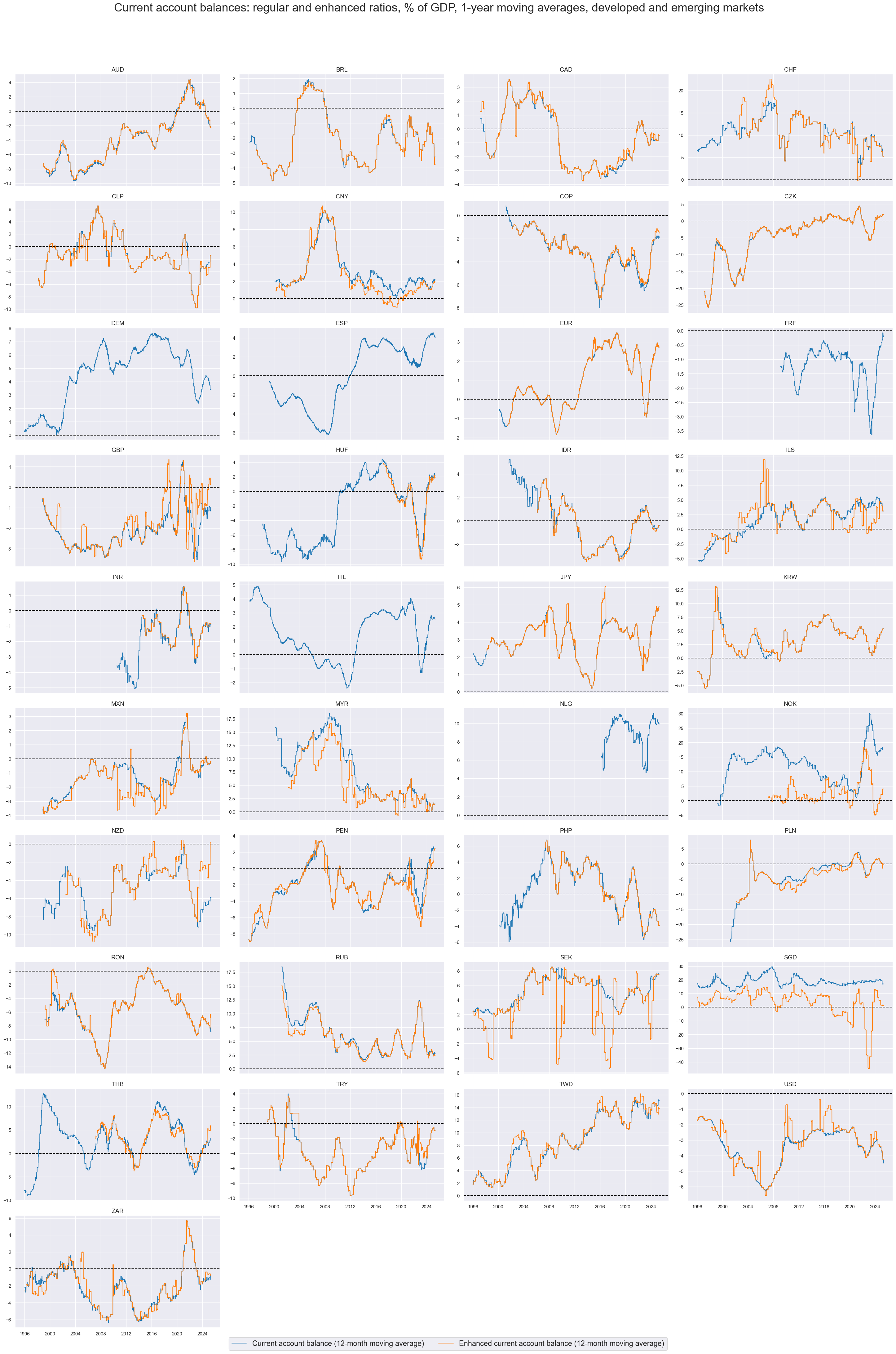
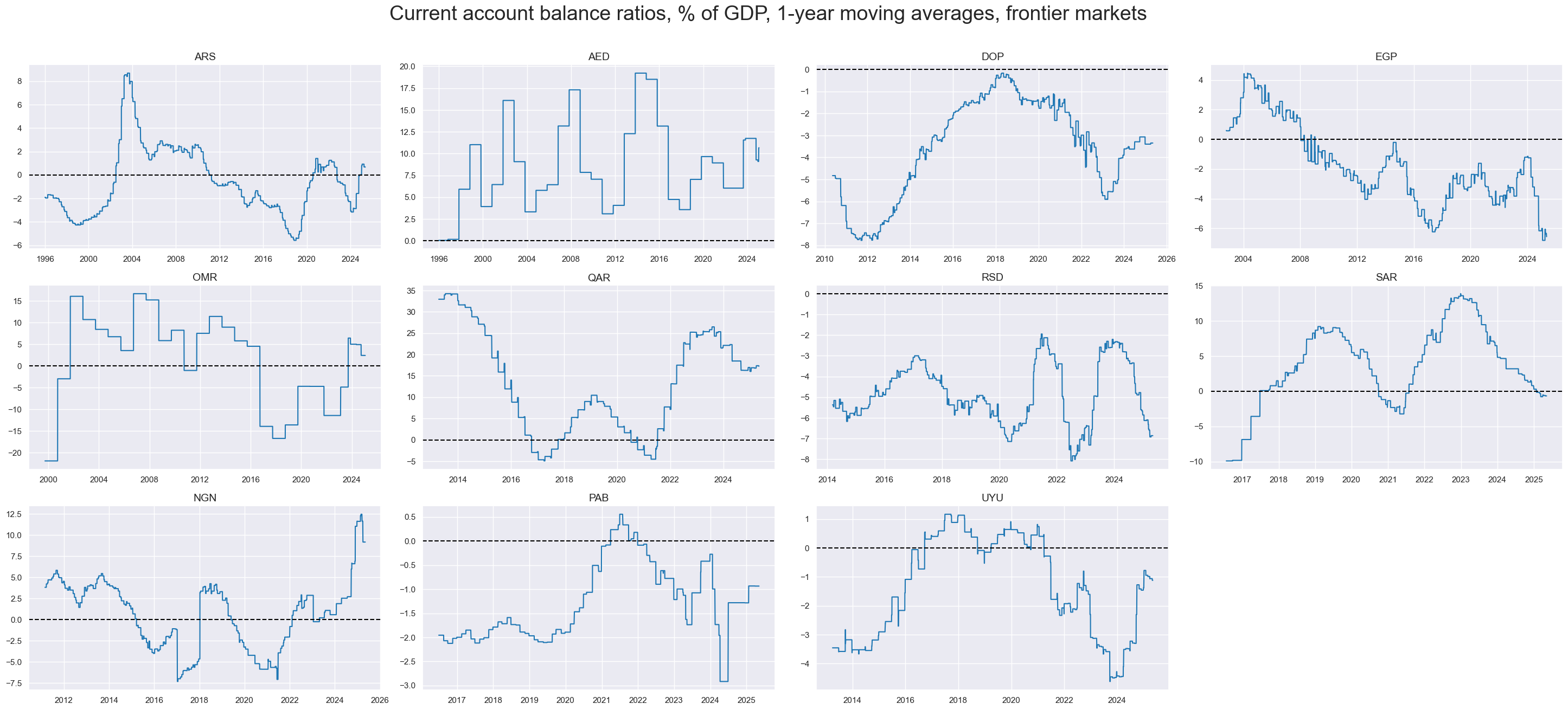
External current account ratios have displayed persistent differences across countries, emphasising their characteristic as slowly-evolving differentiating features. Persistence of external deficits or surpluses reflects a variety of causes, such as government interventions (FX interventions, sovereign wealth funds), evolution of financial relations (long-term credit flows), and unobserved external transactions.
xcatx = ["CABGDPRATIO_NSA_12MMA"]
cidx = cids

msp.view_ranges(
    dfd,
    xcats=xcatx,
    cids=cidx,
    sort_cids_by="mean",
    start=start_date,
    title="Means and standard deviations of external current account ratios since 1996",
    xcat_labels=["External current account, 1-year moving average"],
    kind="bar",
    size=(16, 8),
)
xcatx = ["CABGDPRATIO_NSA_12MMA", "CABGDPRATIOE_NSA_12MMA"]
cidx = sorted(list(set(cids) - set(cids_frontier)))

msp.view_timelines(
    dfd,
    xcats=xcatx,
    cids=cidx,
    start=start_date,
    title="Current account balances: regular and enhanced ratios, % of GDP, 1-year moving averages, developed and emerging markets",
    title_adj=1.02,
    title_xadj=0.49,
    title_fontsize=27,
    legend_fontsize=17,
    xcat_labels=["Current account balance (12-month moving average)", "Enhanced current account balance (12-month moving average)"],
    ncol=4,
    same_y=False,
    size=(16, 8),
    aspect=1.7,
    all_xticks=False,
)
xcatx = ["CABGDPRATIO_NSA_12MMA"]
cidx = cids_frontier

msp.view_timelines(
    dfd,
    xcats=xcatx,
    cids=cidx,
    start=start_date,
    title="Current account balance ratios, % of GDP, 1-year moving averages, frontier markets",
    title_adj=1.02,
    title_xadj=0.49,
    title_fontsize=27,
    legend_fontsize=17,
    xcat_labels=["Current account balance (12-month moving average)"],
    ncol=4,
    same_y=False,
    size=(16, 8),
    aspect=1.7,
    all_xticks=True,
)
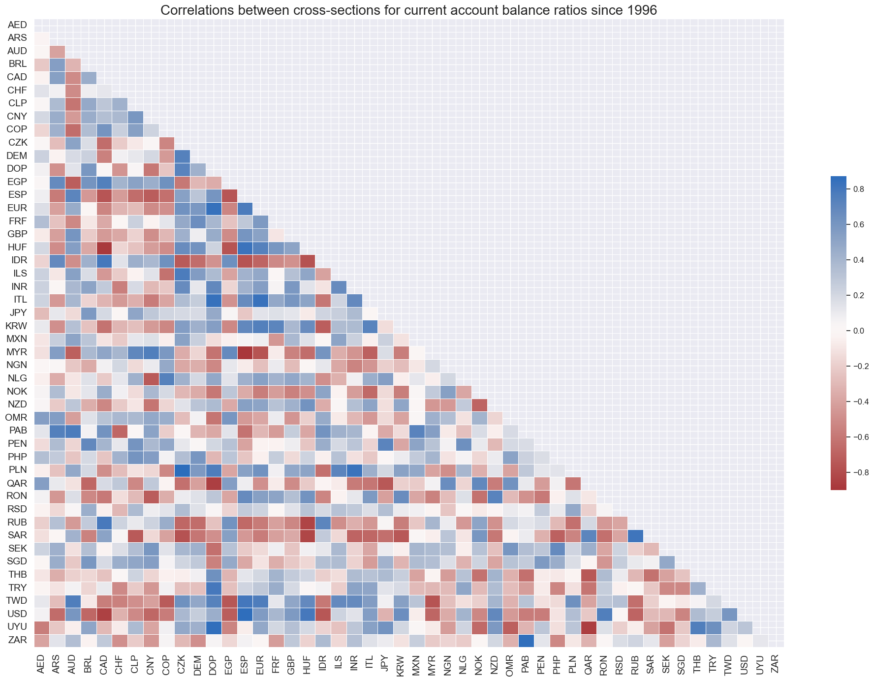
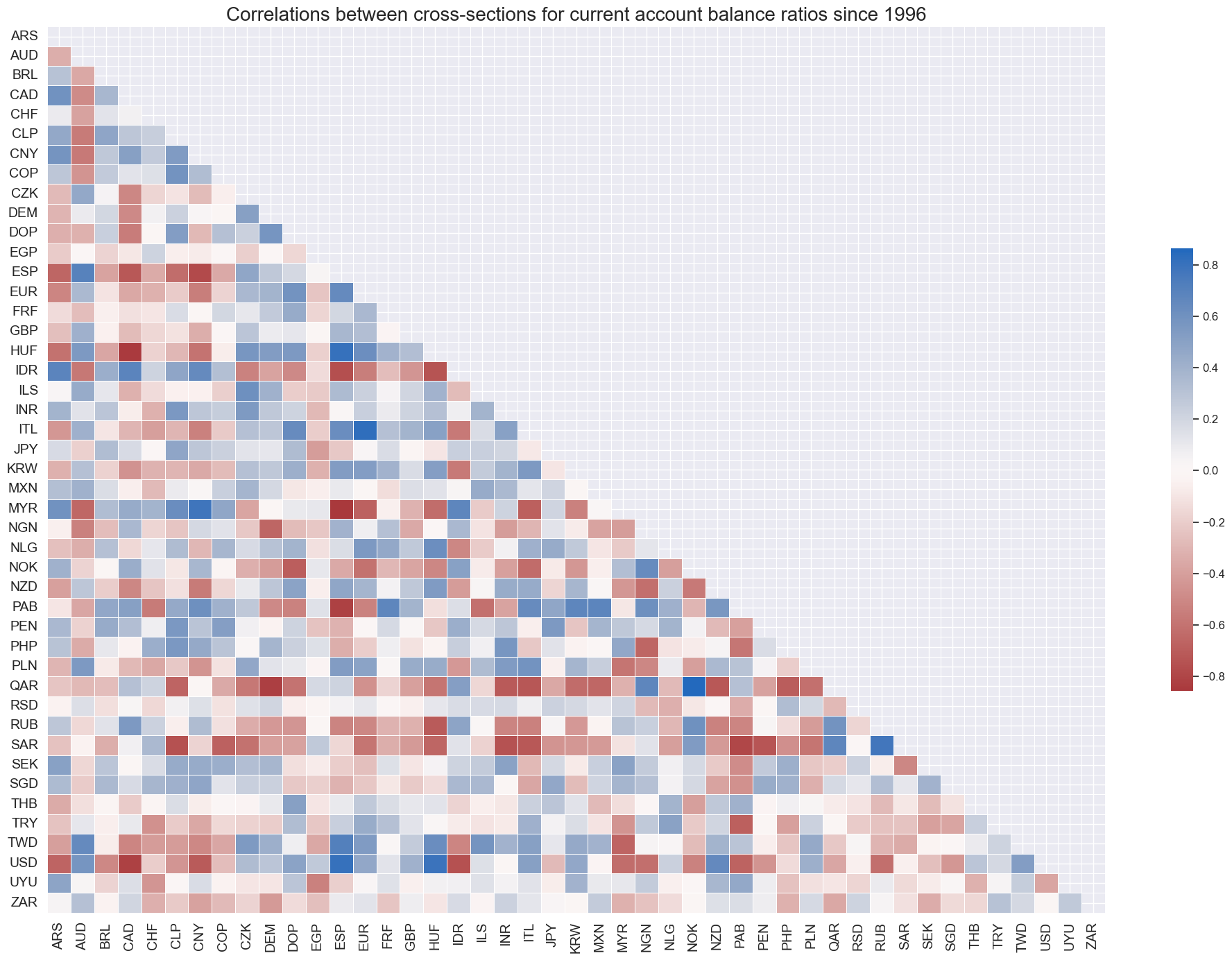
External current account balances are a differentiating macro factor across currency areas.
cidx = cids

msp.correl_matrix(
    dfd,
    xcats="CABGDPRATIO_NSA_12MMA",
    cids=cidx,
    size=(20, 14),
    title="Correlations between cross-sections for current account balance ratios since 1996",
)
Seasonally adjusted external current account ratios #
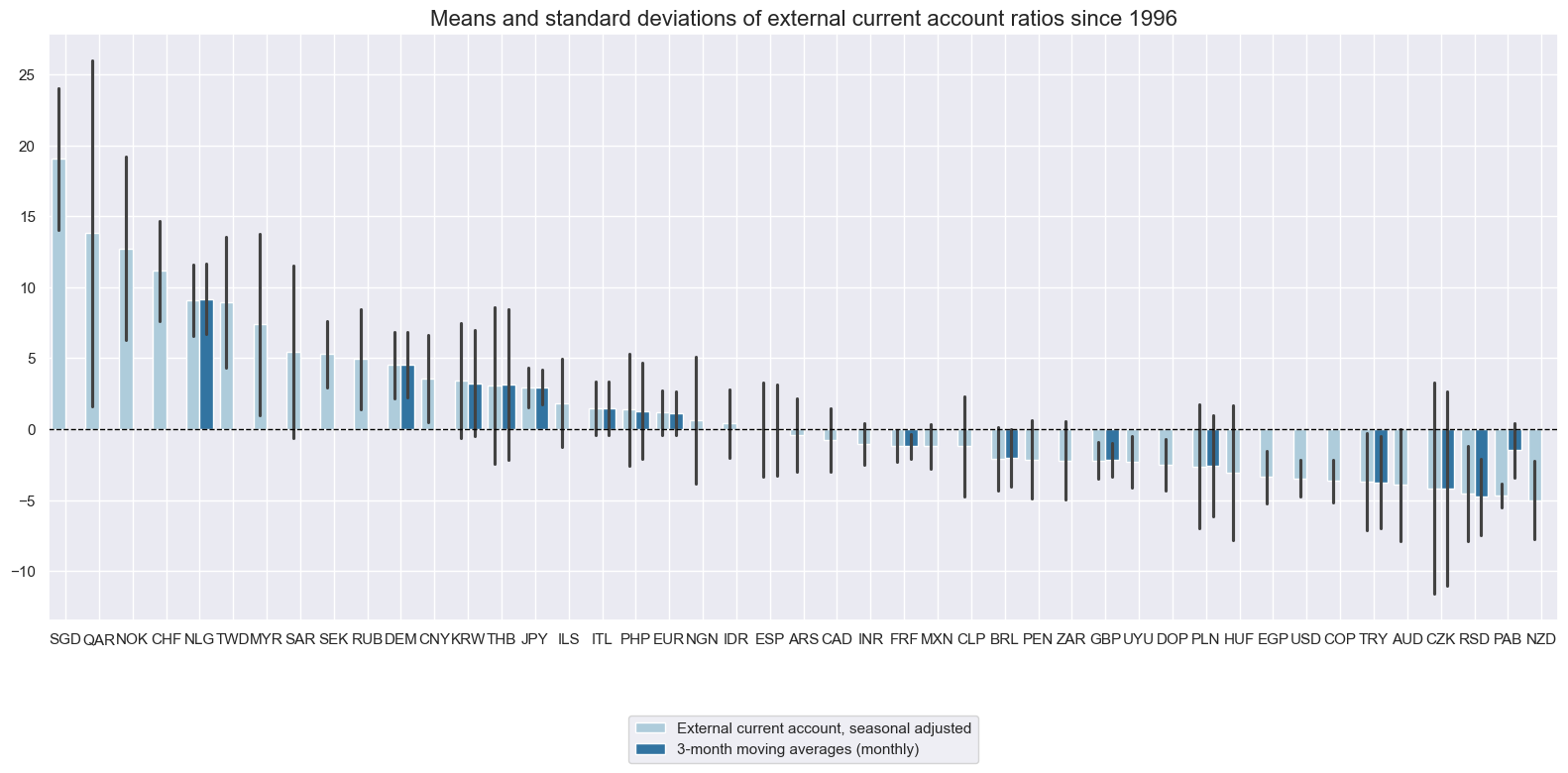
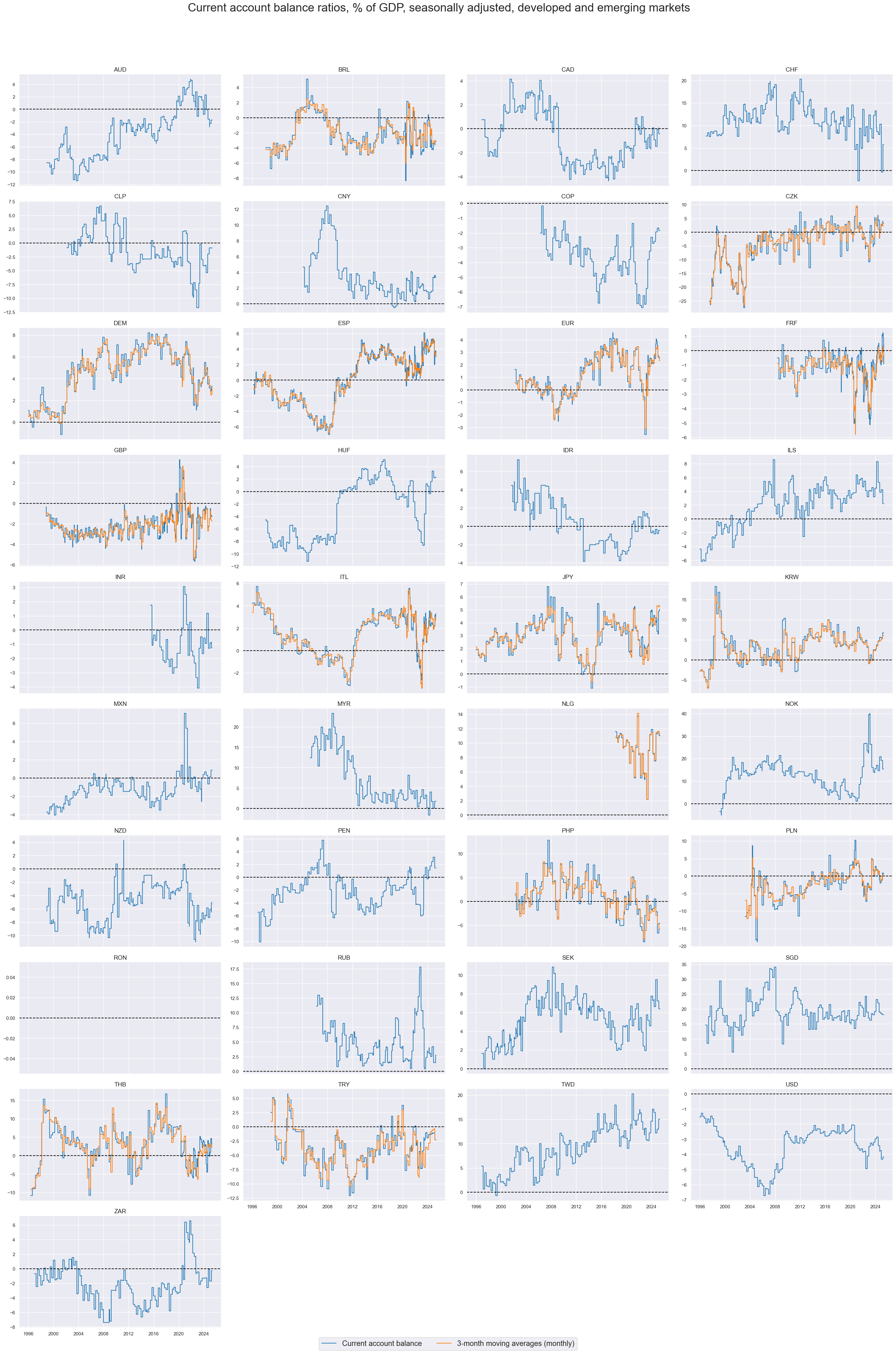
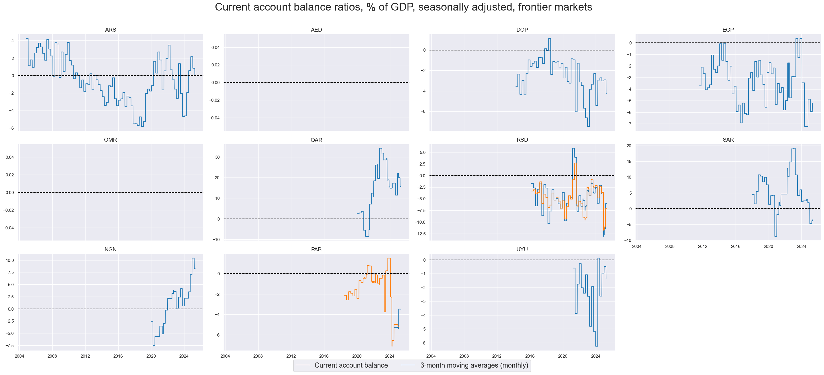
We see a similar pattern in the seasonally adjusted current accounts ratio to the 1-year moving averages, albeit more volatile as is to be expected for monthly and quarterly data flows. The persistence observed in the 1-year trends, are however still clearly visible in the timeseries.
xcatx = ["CABGDPRATIO_SA", "CABGDPRATIO_SA_3MMA"]
cidx = list(set(cids) - set(['OMR']))

msp.view_ranges(
    dfd,
    xcats=xcatx,
    cids=cidx,
    sort_cids_by="mean",
    start=start_date,
    title="Means and standard deviations of external current account ratios since 1996",
    xcat_labels=["External current account, seasonal adjusted", "3-month moving averages (monthly)"],
    kind="bar",
#     size=(16, 8),
)
xcatx = ["CABGDPRATIO_SA", "CABGDPRATIO_SA_3MMA"]
cidx = sorted(list(set(cids) - set(cids_frontier)))

msp.view_timelines(
    dfd,
    xcats=xcatx,
    cids=cidx,
    start=start_date,
    title="Current account balance ratios, % of GDP, seasonally adjusted, developed and emerging markets",
    title_adj=1.02,
    title_xadj=0.49,
    title_fontsize=27,
    legend_fontsize=17,
    xcat_labels=["Current account balance", "3-month moving averages (monthly)"],
    ncol=4,
    same_y=False,
    size=(16, 8),
    aspect=1.7,
    all_xticks=False,
)
xcatx = ["CABGDPRATIO_SA", "CABGDPRATIO_SA_3MMA"]
cidx = cids_frontier

msp.view_timelines(
    dfd,
    xcats=xcatx,
    cids=cidx,
    start=start_date,
    title="Current account balance ratios, % of GDP, seasonally adjusted, frontier markets",
    title_adj=1.02,
    title_xadj=0.49,
    title_fontsize=27,
    legend_fontsize=17,
    xcat_labels=["Current account balance", "3-month moving averages (monthly)"],
    ncol=4,
    same_y=False,
    size=(16, 8),
    aspect=1.7,
    all_xticks=False,
)
Similar to the 1-year trend, the correlation patterns for the seasonal adjusted quarterly (and monthly) balances stays roughly the same, despite higher volaility.
cidx = cids

msp.correl_matrix(
    dfd,
    xcats="CABGDPRATIO_SA",
    cids=cidx,
    size=(20, 14),
    title="Correlations between cross-sections for current account balance ratios since 1996",
)
Merchandise trade balance ratios #
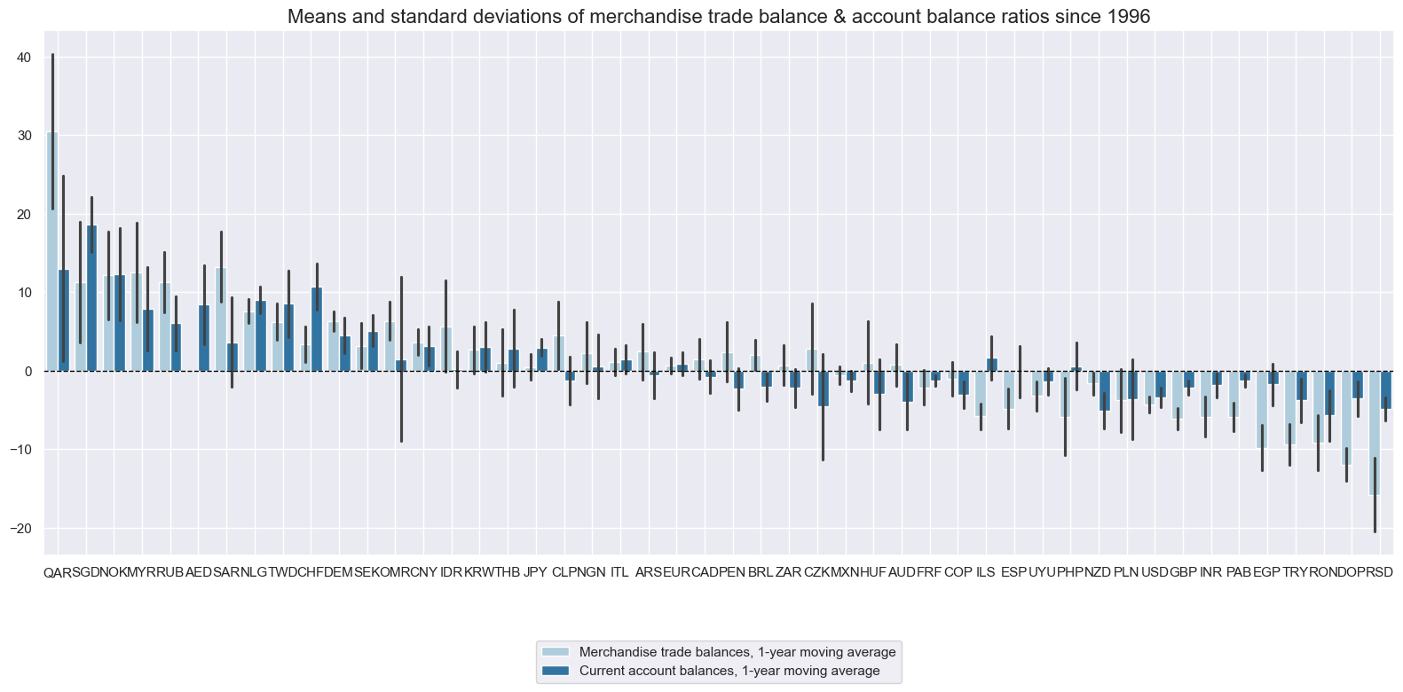
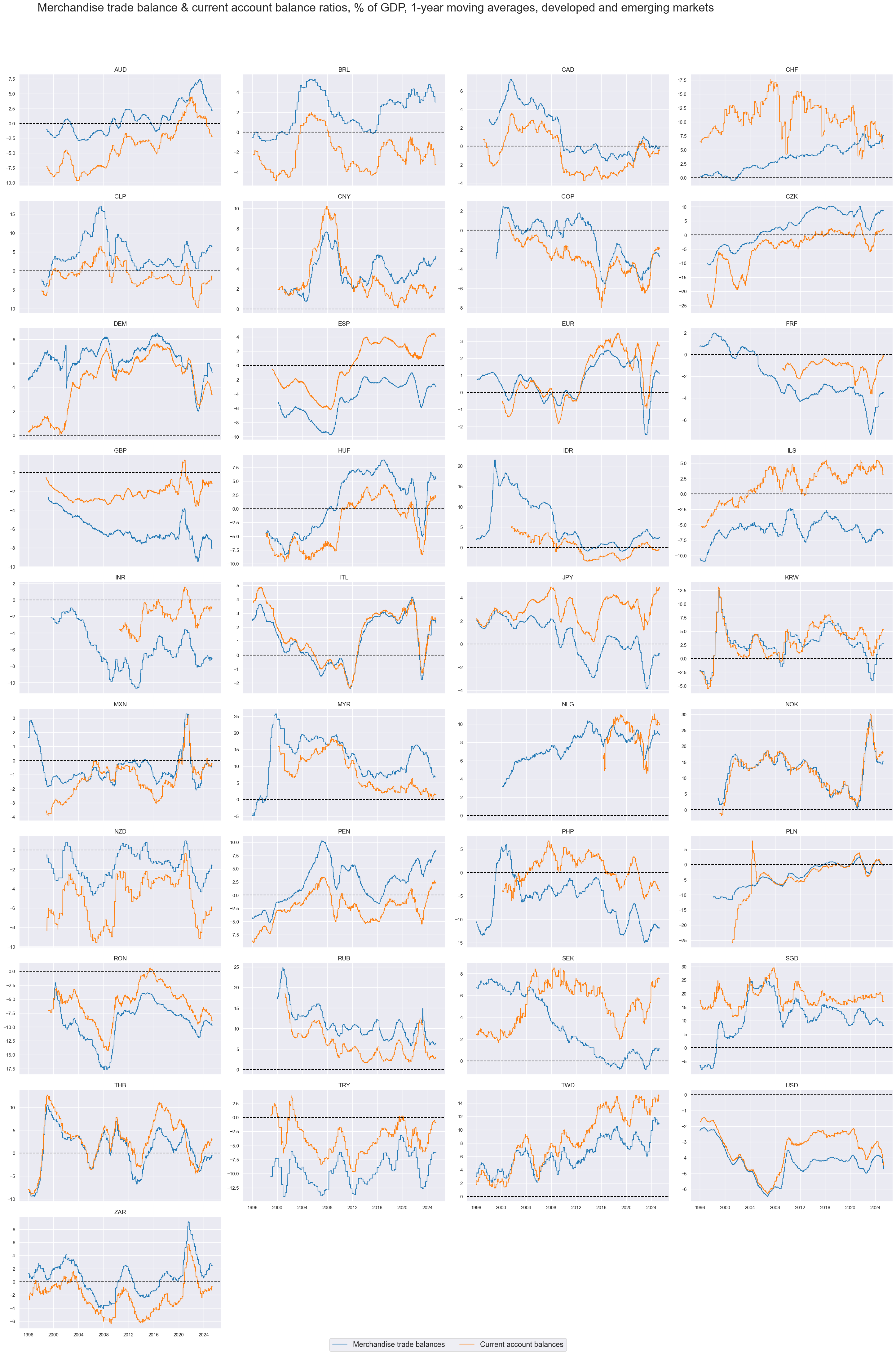
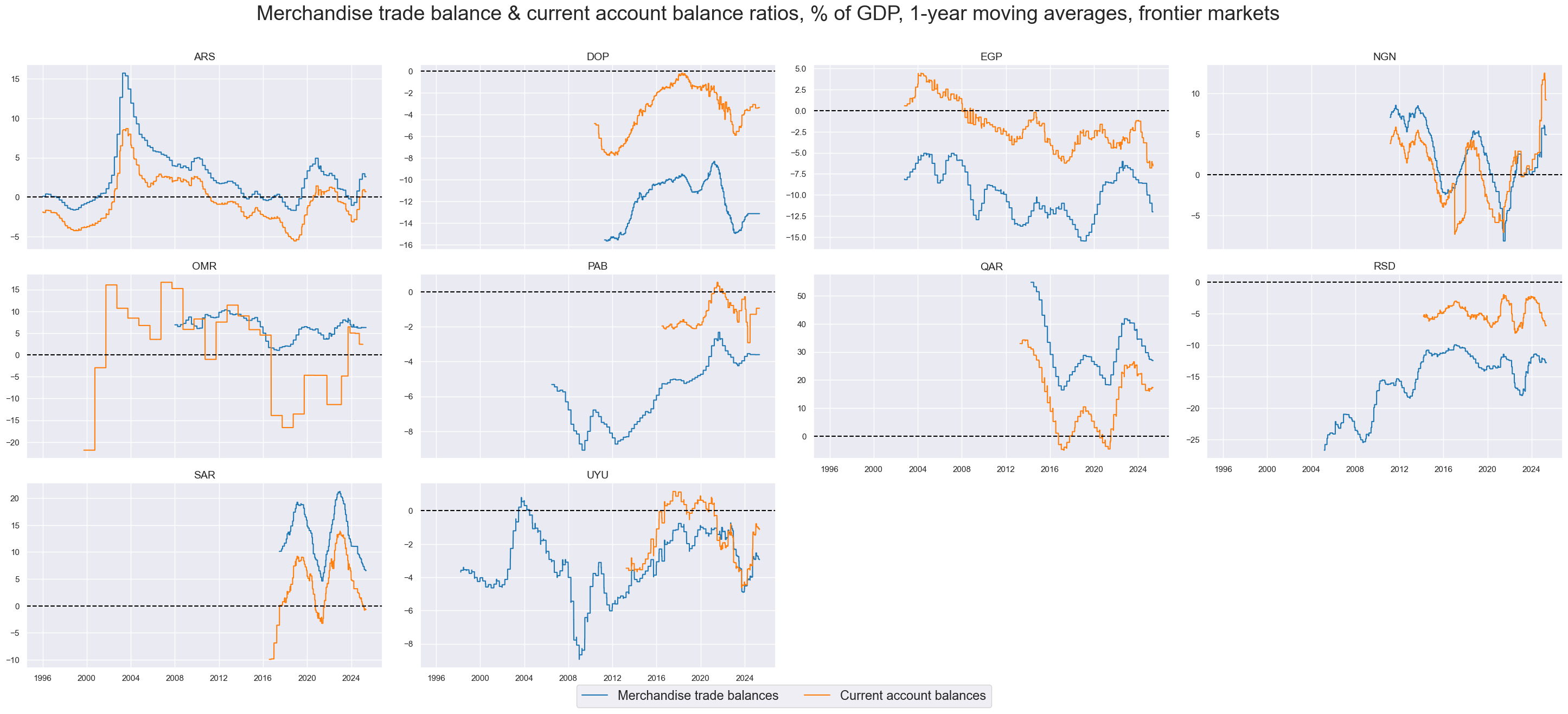
Whilst merchandise and current account balances have naturally been strongly correlated, average levels have displayed disparities for some countries that have a sizable external services trade or net factor income.
xcatx = ["MTBGDPRATIO_NSA_12MMA", "CABGDPRATIO_NSA_12MMA"]
cidx = cids

msp.view_ranges(
    dfd,
    xcats=xcatx,
    cids=cidx,
    sort_cids_by="mean",
    start=start_date,
    title="Means and standard deviations of merchandise trade balance & account balance ratios since 1996",
    xcat_labels=[
        "Merchandise trade balances, 1-year moving average",
        "Current account balances, 1-year moving average",
    ],
    kind="bar",
    size=(16, 8),
)
While external trade balances are slow-moving indicators most of the time, they can change rapidly in times of market turmoil or economic change and - thereby - alter the risk properties of local asset markets.
xcatx = ["MTBGDPRATIO_NSA_12MMA", "CABGDPRATIO_NSA_12MMA"]
cidx = sorted(list(set(cids) - set(cids_frontier)))

msp.view_timelines(
    dfd,
    xcats=xcatx,
    cids=cidx,
    start=start_date,
    title="Merchandise trade balance & current account balance ratios, % of GDP, 1-year moving averages, developed and emerging markets",
    title_adj=1.02,
    title_fontsize=27,
    legend_fontsize=17,
    title_xadj=0.42,
    label_adj=0.075,
    xcat_labels=["Merchandise trade balances", "Current account balances"],
    ncol=4,
    same_y=False,
    size=(16, 8),
    aspect=1.7,
    all_xticks=False,
)
xcatx = ["MTBGDPRATIO_NSA_12MMA", "CABGDPRATIO_NSA_12MMA"]
cidx = sorted(list(set(cids_frontier) - set(['AED'])))

msp.view_timelines(
    dfd,
    xcats=xcatx,
    cids=cidx,
    start=start_date,
    title="Merchandise trade balance & current account balance ratios, % of GDP, 1-year moving averages, frontier markets",
    title_adj=1.02,
    title_xadj=0.49,
    title_fontsize=27,
    legend_fontsize=17,
    xcat_labels=["Merchandise trade balances", "Current account balances"],
    ncol=4,
    same_y=False,
    size=(16, 8),
    aspect=1.7,
    all_xticks=False,
)
Short-term trade balance ratios #
The two short term trade balance ratios appear consistent across currency areas. This extends to extreme observations.
xcatx = ["MTBGDPRATIO_SA_3MMA", "MTBGDPRATIO_SA_6MMA"]
cidx = cids

msp.view_timelines(
    dfd,
    xcats=xcatx,
    cids=cidx,
    start=start_date,
    title="Short-term merchandise balance ratios, % of GDP, seasonally adjusted",
    title_adj=1.02,
    title_fontsize=27,
    legend_fontsize=17,
    label_adj=0.075,
    title_xadj=0.42,
    xcat_labels=["3-month moving average", "6-month moving average"],
    ncol=4,
    same_y=False,
    size=(16, 8),
    aspect=1.7,
    all_xticks=True,
)
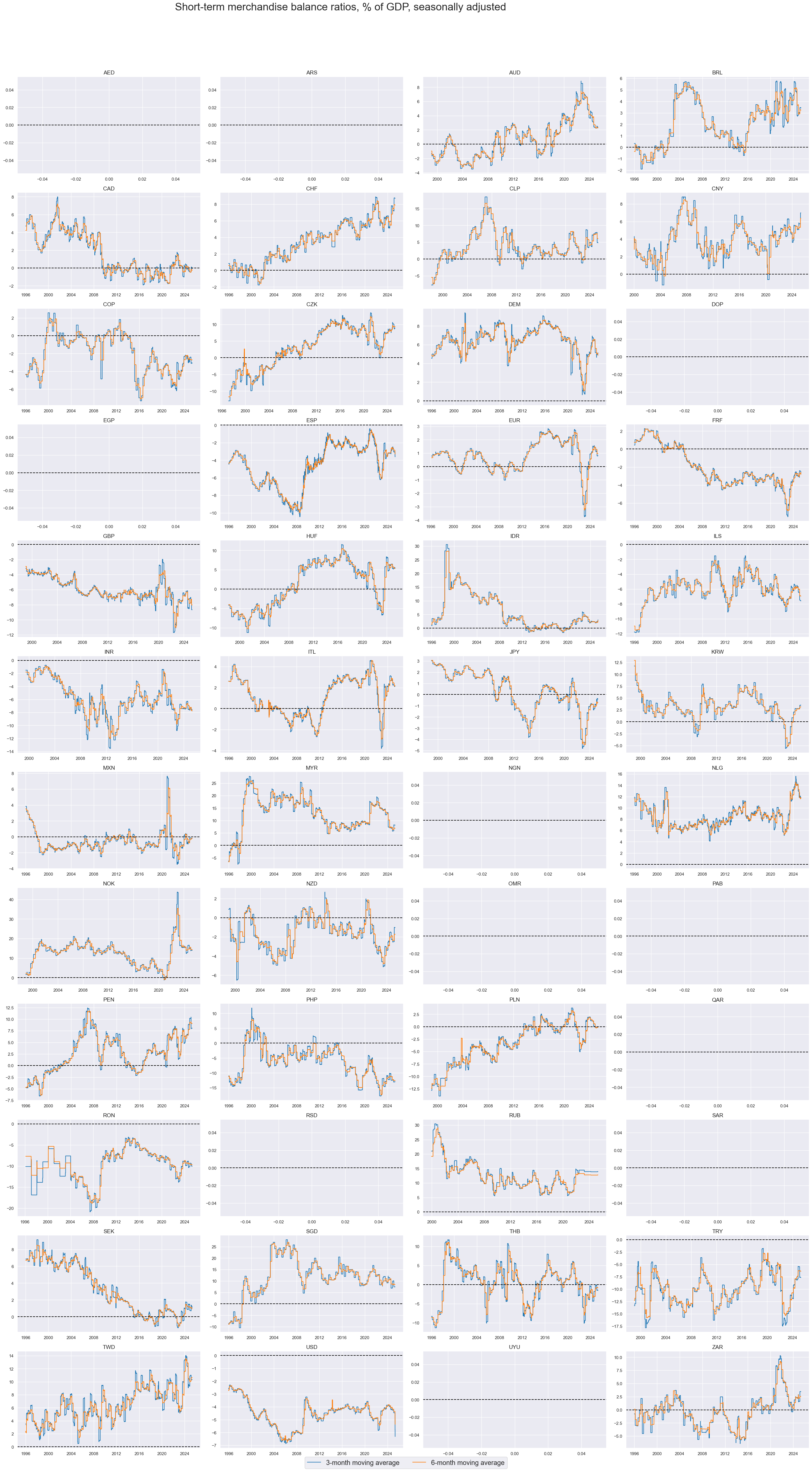
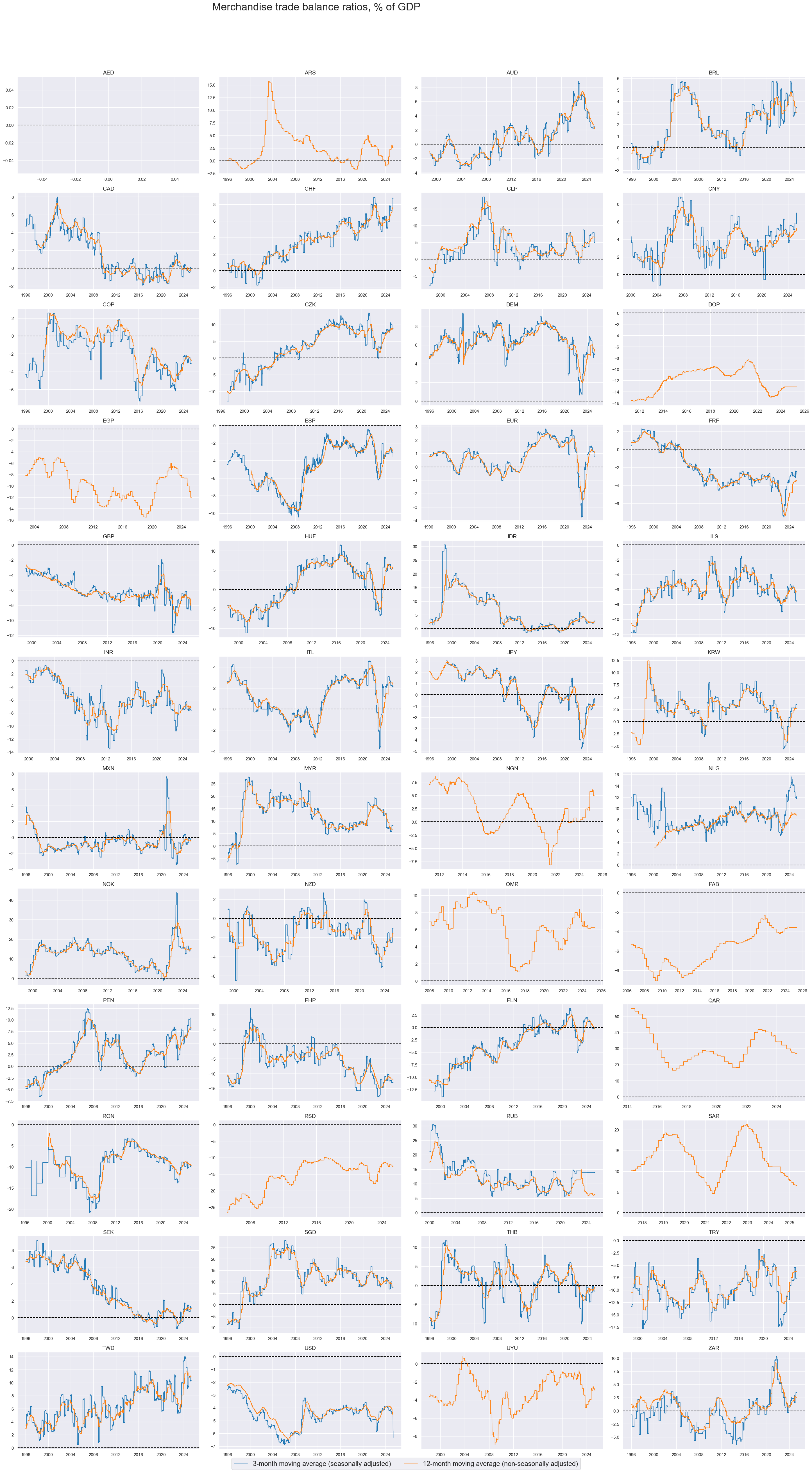
Merchandise trade balance ratios that are based only on a few months of seasonally adjusted data are typically leading the traditional 12-month ratios at the expense of ample added volatility. The short-term ratios are better indicators of external adjustments to economic shocks, while the longer-horizon ratios better reflect medium-term trends.
xcatx = ["MTBGDPRATIO_SA_3MMA", "MTBGDPRATIO_NSA_12MMA"]
cidx = cids

msp.view_timelines(
    dfd,
    xcats=xcatx,
    cids=cidx,
    start=start_date,
    title="Merchandise trade balance ratios, % of GDP",
    title_adj=1.02,
    title_xadj=0.39,
    title_fontsize=27,
    legend_fontsize=17,
    label_adj=0.075,
    xcat_labels=[
        "3-month moving average (seasonally adjusted)",
        "12-month moving average (non-seasonally adjusted)",
    ],
    ncol=4,
    same_y=False,
    size=(16, 8),
    aspect=1.7,
    all_xticks=True,
)
Net FDI ratios #
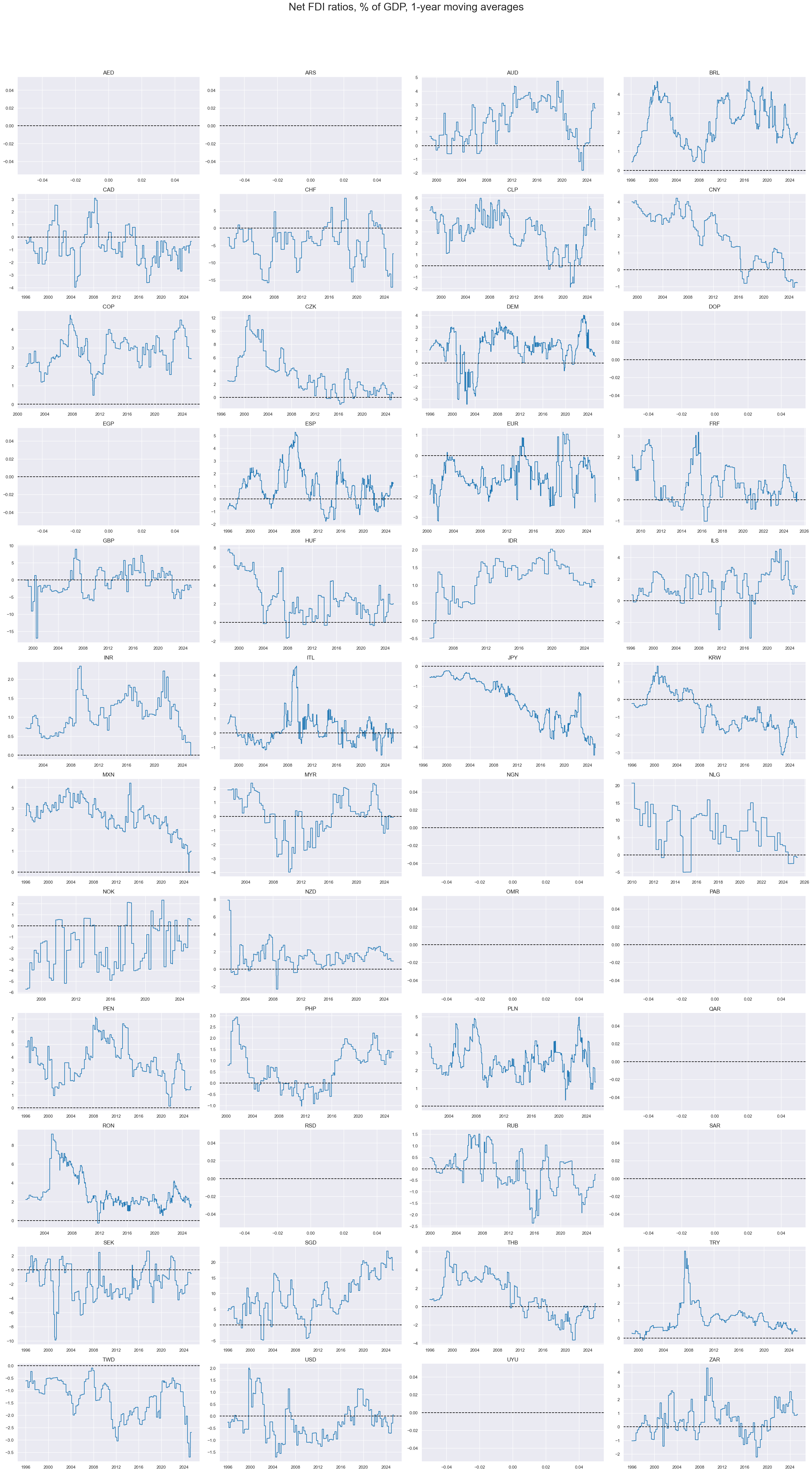
Net FDI ratios exhibit greater variability than trade balances, notwithstanding the exclusion of monthly outliers in our calculations. On balance, EM economies have been recipients of net currency demand for foreign direct investment purposes.
xcatx = ["NFDIGDPRATIO_NSA_12MMA"]
cidx = cids

msp.view_timelines(
    dfd,
    xcats=xcatx,
    cids=cidx,
    start=start_date,
    title="Net FDI ratios, % of GDP, 1-year moving averages",
    title_adj=1.02,
    title_fontsize=27,
    title_xadj=0.5,
    ncol=4,
    same_y=False,
    size=(16, 8),
    aspect=1.7,
    all_xticks=True,
)
Basic external balance ratios #
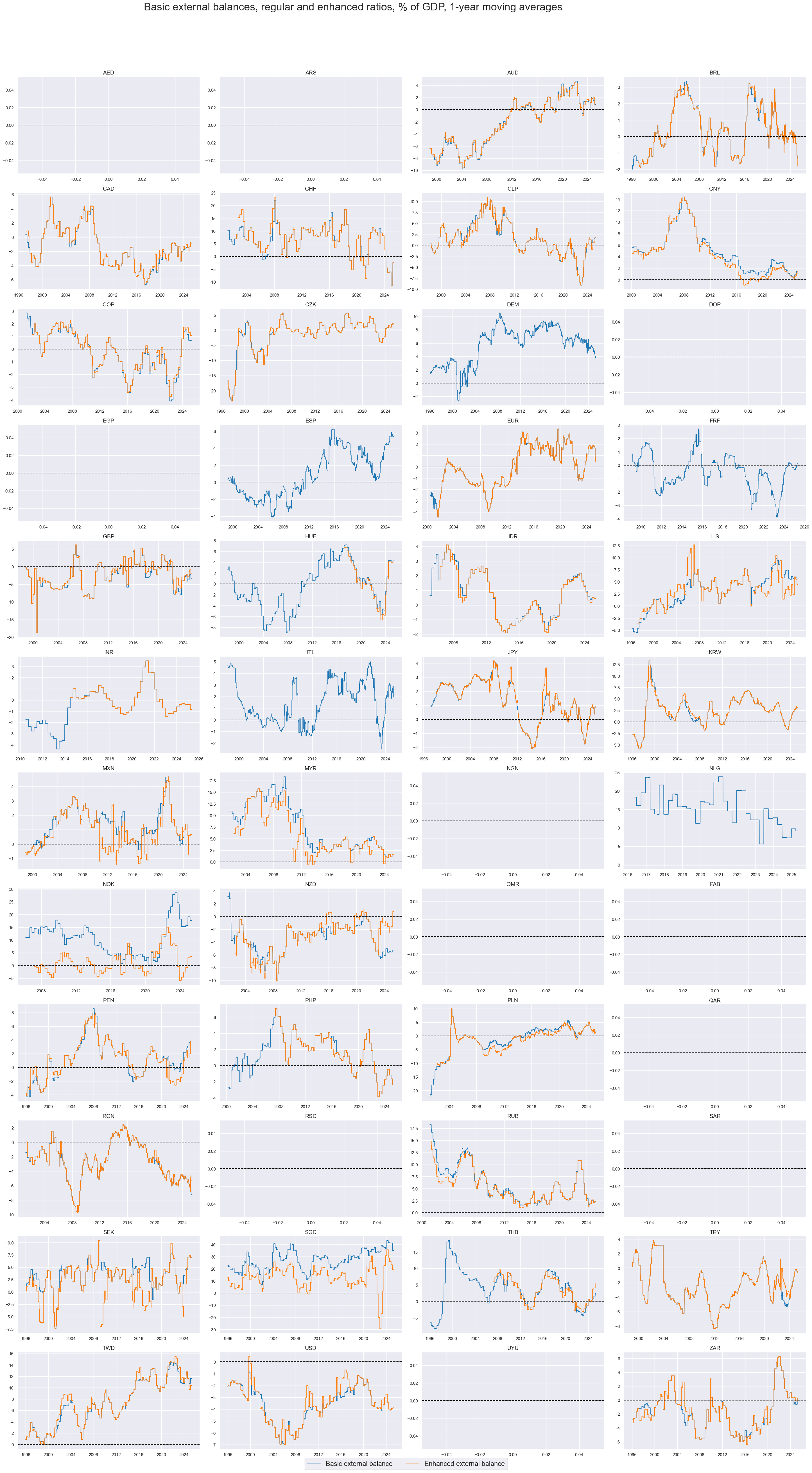
Basic external balances are the broadest concepts of external in and outflows. The enhanced concept does not only consider net foreign direct investments, but also stable flows from sovereign wealth funds and net errors and omissions. For most countries the effects of the enhancement are modest However, for Singapore, and Norway, enhanced external balances have deviated substantially from basic external balances in the long run. For others differences have been episodic.
xcatx = ["BXBGDPRATIO_NSA_12MMA", "BXBGDPRATIOE_NSA_12MMA"]
cidx = cids

msp.view_timelines(
    dfd,
    xcats=xcatx,
    cids=cidx,
    start=start_date,
    title="Basic external balances, regular and enhanced ratios, % of GDP, 1-year moving averages",
    xcat_labels=[
        "Basic external balance",
        "Enhanced external balance",
    ],
    title_adj=1.02,
    title_fontsize=27,
    legend_fontsize=17,
    title_xadj=0.435,
    label_adj=0.075,
    ncol=4,
    same_y=False,
    size=(16, 8),
    aspect=1.7,
    all_xticks=True,
)
Net foreign portfolio investment-to-GDP ratios #
Average net foreign portfolio investment-to-GDP ratios have been diverse across countries. Generally, countries with large external current account surpluses and sovereign wealth funds have recorded large outflows.
xcatx = ["NFPIGDPRATIO_NSA_4QMA"]
cidx = cids

msp.view_ranges(
    dfd,
    xcats=xcatx,
    cids=cidx,
    sort_cids_by="mean",
    start=start_date,
    title="Means and standard deviations of net foreign portfolio investment ratios since 1996",
    xcat_labels=["Net foreign portfolio investment, 4-quarter moving average",],
    kind="bar",
    size=(16, 8),
)
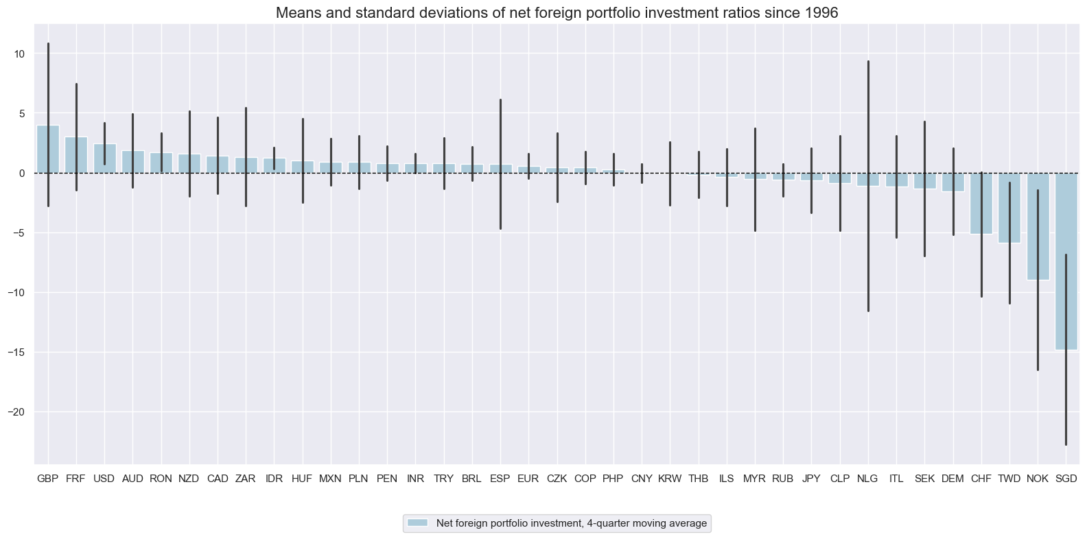
Although net external portfolio flows have been notoriously volatile, they also have displayed pronounced cycles and medium-term trends.
xcatx = ["NFPIGDPRATIO_NSA_4QMA", "NFPIGDPRATIO_NSA_2QMA", "NFPIGDPRATIO_NSA"]
cidx = cids

msp.view_timelines(
    dfd,
    xcats=xcatx,
    cids=cidx,
    start=start_date,
    title="Net foreign portfolio investment ratios, % of GDP",
    title_adj=1.02,
    title_fontsize=30,
    legend_fontsize=17,
    title_xadj=0.435,
    label_adj=0.075,
    ncol=4,
    same_y=False,
    size=(16, 8),
    xcat_labels=[
        "Net foreign portfolio investment, 4-quarter moving average",
        "Net foreign portfolio investment, 2-quarter moving average",
        "Net foreign portfolio investment",
    ],
    aspect=1.7,
    all_xticks=True,
)
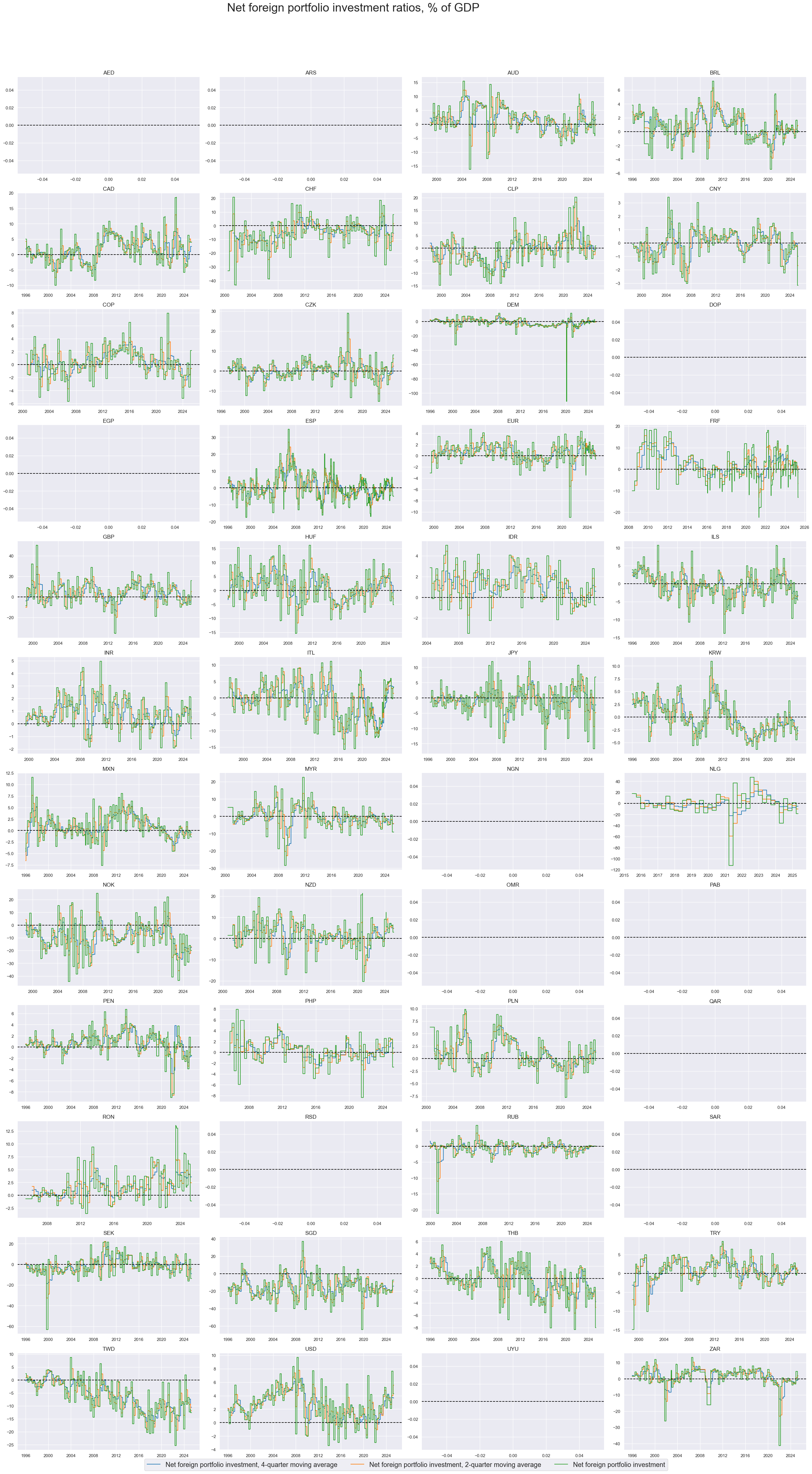
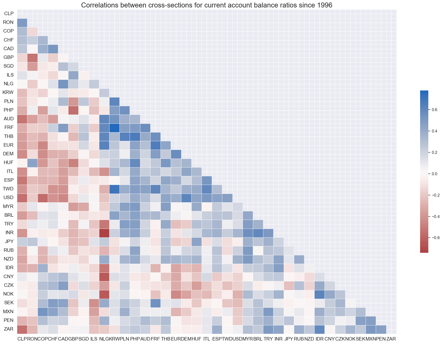
Correlations of net portfolio flows of countries have been very diverse, suggesting that this a diversifying factor in a global portfolio.
cidx = cids

msp.correl_matrix(
    dfd,
    xcats="NFPIGDPRATIO_NSA_4QMA",
    cids=cidx,
    size=(20, 14),
    title="Correlations between cross-sections for current account balance ratios since 1996",
    cluster=True,
)
Net foreign lending investment-to-GDP ratios #
The long-term averages in net lending have been less diverse than those for net portfolio investment and relative to volatility.
xcatx = ["NFLGDPRATIO_NSA_4QMA"]
cidx = cids

msp.view_ranges(
    dfd,
    xcats=xcatx,
    cids=cidx,
    sort_cids_by="mean",
    start=start_date,
    title="Means and standard deviations of net foreign lending ratios since 1996",
    xcat_labels=["Net foreign lending, 4-quarter moving average"],
    kind="bar",
    size=(16, 8),
)
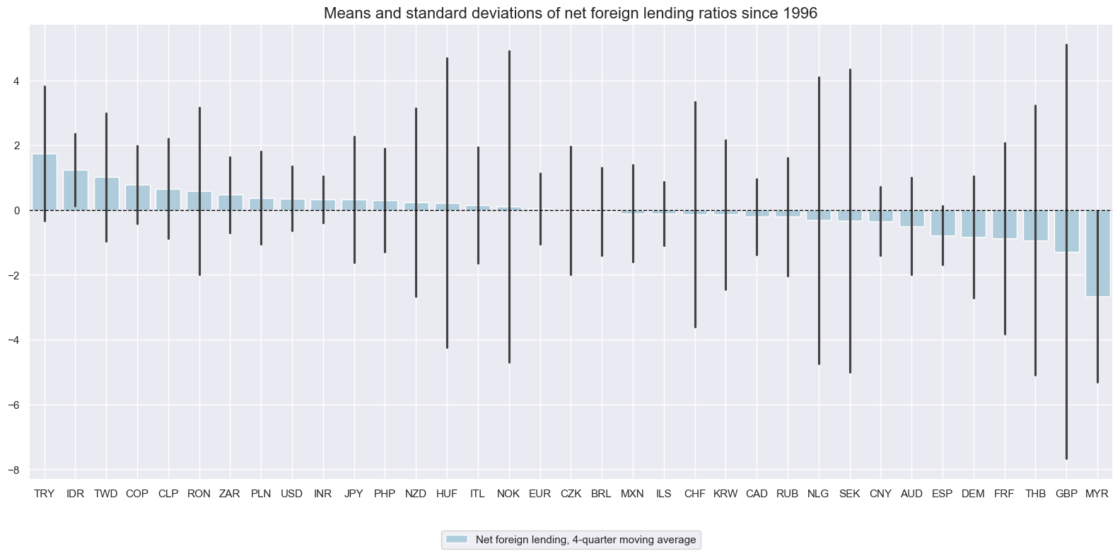
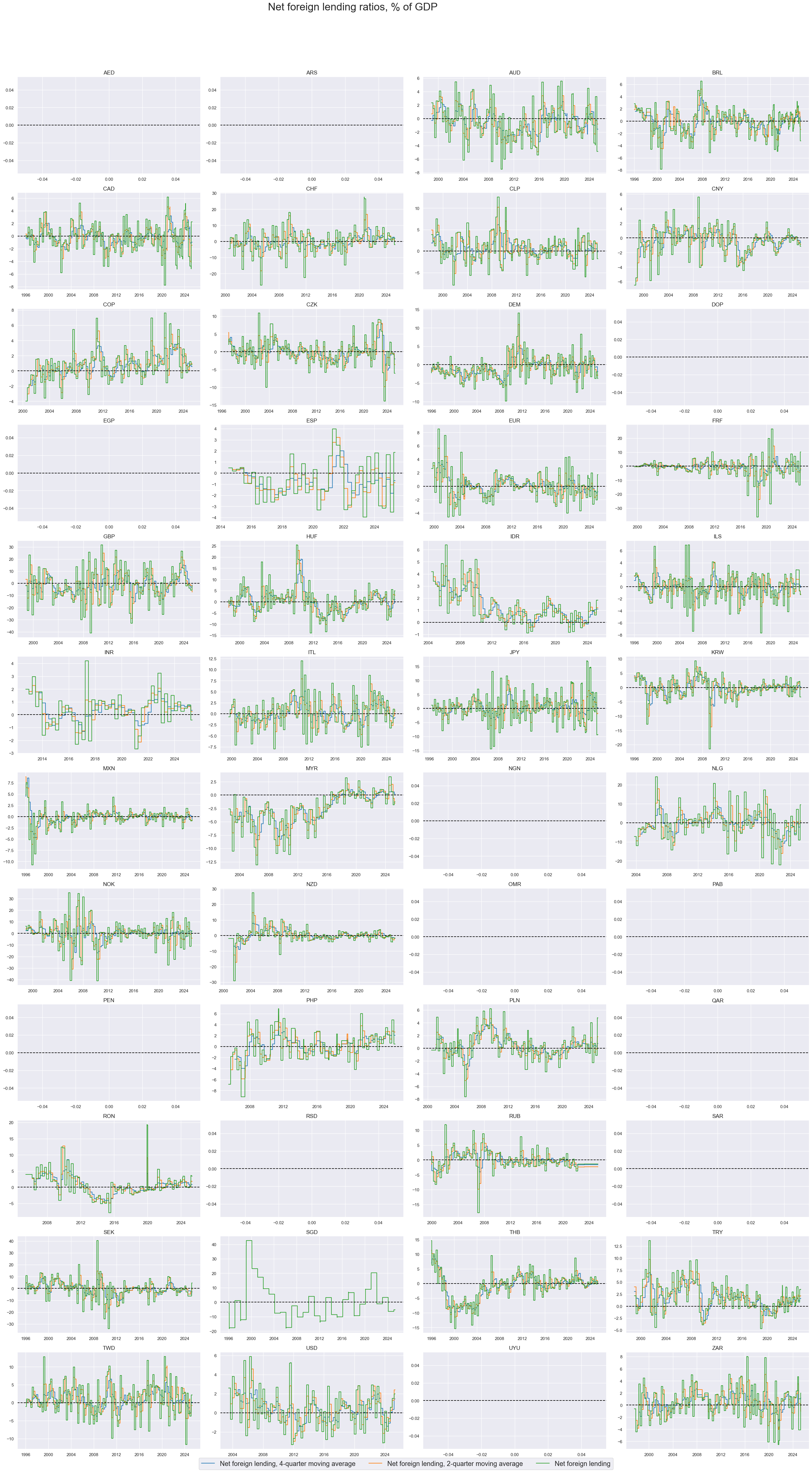
Beyond volatility, the net lending ratios have also displayed cycles and sometimes structural trends and shifts.
xcatx = ["NFLGDPRATIO_NSA_4QMA", "NFLGDPRATIO_NSA_2QMA", "NFLGDPRATIO_NSA"]

cidx = cids


msp.view_timelines(
    dfd,
    xcats=xcatx,
    cids=cidx,
    start=start_date,
    title="Net foreign lending ratios, % of GDP",
    title_adj=1.02,
    title_fontsize=27,
    legend_fontsize=17,
    title_xadj=0.435,
    label_adj=0.075,
    ncol=4,
    same_y=False,
    size=(16, 8),
    xcat_labels=[
        "Net foreign lending, 4-quarter moving average",
        "Net foreign lending, 2-quarter moving average",
        "Net foreign lending",
    ],

    aspect=1.7,
    all_xticks=True,

)
Importance #
Research links #
“Backtesting exercises show that although both metrics are noisy, the basic balance is a better leading indicator of FX returns than the current account balance, particularly in EM.” Chandan/JPMorgan
“External balance and FX carry (nominal or real) tend to be negatively correlated, so in effect, one is short carry when long surplus vs. deficit currencies. This provides diversification opportunities in a multi-factor context. Simply a combination of two factors—carry and growth or carry and external balances—is adequate to boost FX risk-adjusted returns.” Chandan, Duran-Vara/ JPMorgan
“Currency areas with negative external balances are – all other things equal – more vulnerable to financing shocks. Jumps in market price volatility often indicate such shocks. Realistically it takes a few days for the market to fully price the consequences of shocks consistently across currencies. Hence, the products of external balances-based “resilience scores” and volatility shocks are plausible indicators of “post-shock currency hazards”. This means that they should serve as signals for differences in currency returns after market volatility has surged or dropped. An empirical analysis based on 28 currencies since 2000 shows that a most simple “post-shock currency hazard” measure has significantly helped predict subsequent short-term returns and would have added positive PnL to FX trading strategies, particularly in times of turbulence.” Macrosynergy
“The current account occupies a central position in international economics and policy debates. Indeed, in G20 policy debates the term ‘global imbalances’ is treated as almost synonymous with ‘current account imbalances’.” Borio
“Countries whose currencies will be most vulnerable…are those that have the largest external financing needs. One simple gauge of this vulnerability is the size of the country’s basic external balance as a share of GDP, i.e., the current account deficit minus the stable sources of financing such as net FDI inflows and (for EU member countries) inflows of EU convergence and cohesion funds.” AllianceBernstein
“There is clear evidence that for emerging market economies that experience large bond outflows, their exchange rates subsequently depreciate significantly, generating large negative currency excess returns.” Hördahl, Valente BIS Working Papers
Empirical clues #
External deficits have historically been a counterweight to (real and nominal) FX carry. Often, high-carry countries compensate investors for helping them to sustain an elevated currency value in the face of external deficits and low-carry countries compensate investors for helping them to prevent currency appreciation in the face of external surpluses.
dfb = dfd[dfd["xcat"].isin(["FXTARGETED_NSA", "FXUNTRADABLE_NSA"])].loc[
    :, ["cid", "xcat", "real_date", "value"]
]
dfba = (
    dfb.groupby(["cid", "real_date"])
    .aggregate(value=pd.NamedAgg(column="value", aggfunc="max"))
    .reset_index()
)
dfba["xcat"] = "FXBLACK"
fxblack = msp.make_blacklist(dfba, "FXBLACK")
fxblack
{'BRL': (Timestamp('2012-12-03 00:00:00'), Timestamp('2013-09-30 00:00:00')),
 'CHF': (Timestamp('2011-10-03 00:00:00'), Timestamp('2015-01-30 00:00:00')),
 'CNY': (Timestamp('1999-01-01 00:00:00'), Timestamp('2025-05-07 00:00:00')),
 'CZK': (Timestamp('2014-01-01 00:00:00'), Timestamp('2017-07-31 00:00:00')),
 'ILS': (Timestamp('1999-01-01 00:00:00'), Timestamp('2005-12-30 00:00:00')),
 'INR': (Timestamp('1999-01-01 00:00:00'), Timestamp('2004-12-31 00:00:00')),
 'MYR_1': (Timestamp('1999-01-01 00:00:00'), Timestamp('2007-11-30 00:00:00')),
 'MYR_2': (Timestamp('2018-07-02 00:00:00'), Timestamp('2025-05-07 00:00:00')),
 'PEN': (Timestamp('2021-07-01 00:00:00'), Timestamp('2021-07-30 00:00:00')),
 'RON': (Timestamp('1999-01-01 00:00:00'), Timestamp('2005-11-30 00:00:00')),
 'RUB_1': (Timestamp('1999-01-01 00:00:00'), Timestamp('2005-11-30 00:00:00')),
 'RUB_2': (Timestamp('2022-02-01 00:00:00'), Timestamp('2025-05-07 00:00:00')),
 'SGD': (Timestamp('1999-01-01 00:00:00'), Timestamp('2025-05-07 00:00:00')),
 'THB': (Timestamp('2007-01-01 00:00:00'), Timestamp('2008-11-28 00:00:00')),
 'TRY_1': (Timestamp('1999-01-01 00:00:00'), Timestamp('2003-09-30 00:00:00')),
 'TRY_2': (Timestamp('2020-01-01 00:00:00'), Timestamp('2024-07-31 00:00:00'))}
cidx = cids_fx

cr = msp.CategoryRelations(
    dfd,
    xcats=["CABGDPRATIOE_NSA_12MMA", "FXCRR_NSA"],
    cids=cidx,
    blacklist=fxblack,
    freq="M",
    lag=0,
    xcat_aggs=["mean", "mean"],
    start=start_date,
    years=3,
)
cr.reg_scatter(
    title="Current account ratios and real FX forward carry across all countries, 3-year periods since 1996",
    labels=True,
    coef_box="upper right",
    ylab="Real 1-month forward-implied FX carry",
    xlab="Current account ratio as % of GDP, 1-year moving average",
    reg_robust=True,
  )
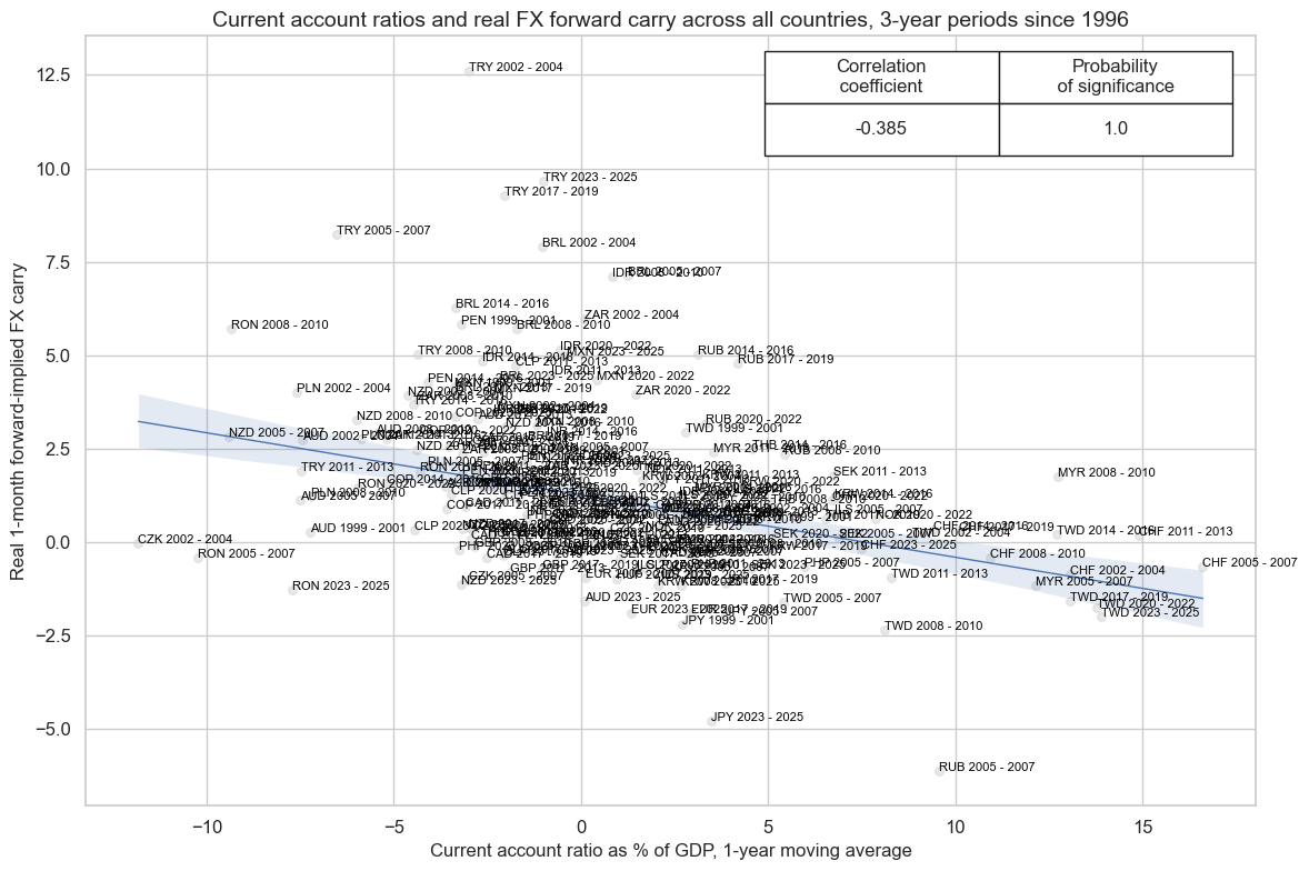
Pooled OLS regression shows a highly significant positive intercept, implying that the current account-to-GDP ratio has to be relatively large before the expected real 1-month FX forward carry is negative.
cr.ols_table()
                            OLS Regression Results
==============================================================================
Dep. Variable:              FXCRR_NSA   R-squared:                       0.148
Model:                            OLS   Adj. R-squared:                  0.144
Method:                 Least Squares   F-statistic:                     37.51
Date:                Thu, 08 May 2025   Prob (F-statistic):           4.24e-09
Time:                        16:50:22   Log-Likelihood:                -477.01
No. Observations:                 218   AIC:                             958.0
Df Residuals:                     216   BIC:                             964.8
Df Model:                           1
Covariance Type:            nonrobust
==========================================================================================
                             coef    std err          t      P>|t|      [0.025      0.975]
------------------------------------------------------------------------------------------
const                      1.4819      0.147     10.054      0.000       1.191       1.772
CABGDPRATIOE_NSA_12MMA    -0.1881      0.031     -6.125      0.000      -0.249      -0.128
==============================================================================
Omnibus:                       60.709   Durbin-Watson:                   1.215
Prob(Omnibus):                  0.000   Jarque-Bera (JB):              169.044
Skew:                           1.193   Prob(JB):                     1.96e-37
Kurtosis:                       6.594   Cond. No.                         4.82
==============================================================================

Notes:
[1] Standard Errors assume that the covariance matrix of the errors is correctly specified.
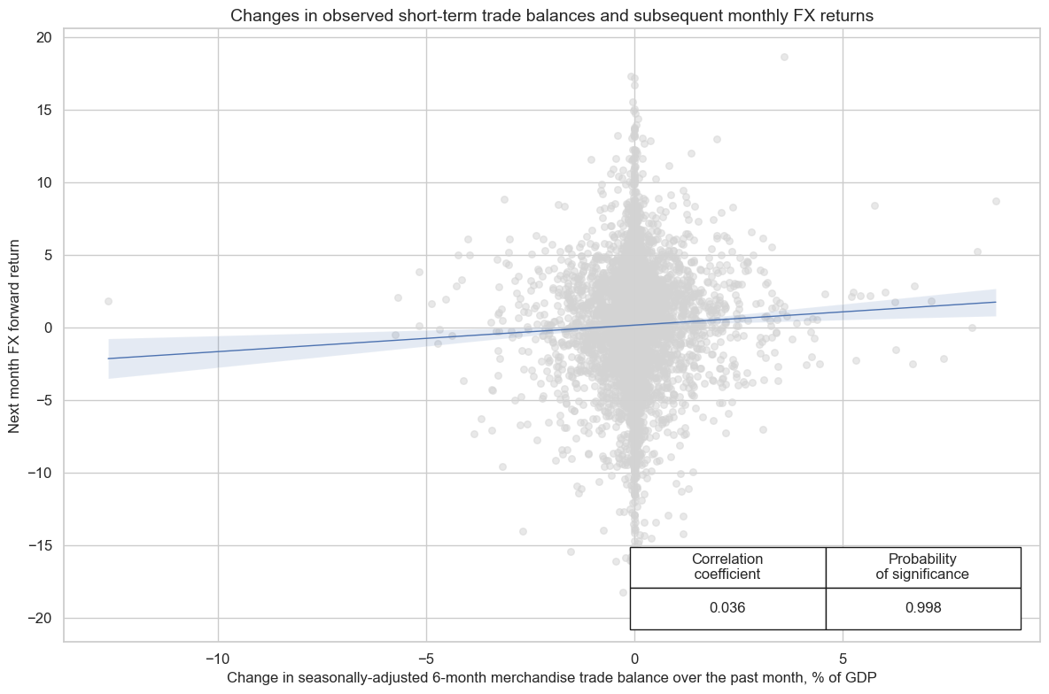
There has been a positive relation between changes in the observed short-term trade balance ratios and subsequent FX returns.
cidx = cids_fx

cr = msp.CategoryRelations(
    dfd,
    xcats=["MTBGDPRATIO_SA_6MMA", "FXXR_VT10"],
    cids=cidx,
    blacklist=fxblack,
    freq="M",
    lag=1,
    xcat_aggs=["last", "sum"],
    xcat1_chg="diff",
    xcat_trims=[20, 20],
    n_periods=1,
    start=start_date,
    years=None,
)
cr.reg_scatter(
    title="Changes in observed short-term trade balances and subsequent monthly FX returns",
    labels=False,
    coef_box="lower right",
    xlab="Change in seasonally-adjusted 6-month merchandise trade balance over the past month, % of GDP",
    ylab="Next month FX forward return",
    prob_est="map",
)
Focusing on a subset of ‘credit countries’ which include nations that are more exposed to credit defaults, positive account balance changes are strongly correlated with the performance of those countries’ foreign currency bond returns.
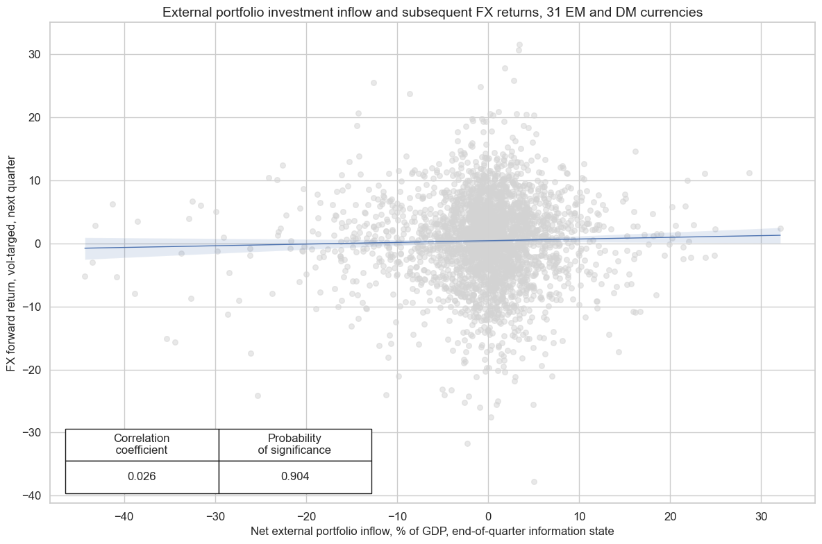
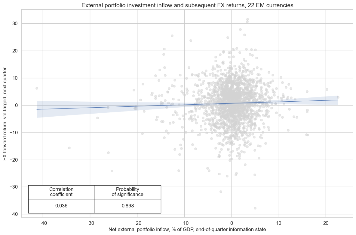
Net portfolio flows have displayed persistent medium-term trends in the past. As a result, we also see a subtle but statistically significant relation between net portfolio flows and subsequent (volatility-targeted) FX returns for a wide panel of 31 emerging and developed currency areas.
cidx = cids_fx

cr = msp.CategoryRelations(
    dfd,
    xcats=["NFPIGDPRATIO_NSA", "FXXR_VT10"],
    cids=cidx,
    blacklist=fxblack,
    freq="q",
    lag=1,
    xcat_aggs=["last", "sum"],
    start=start_date,
    years=None,
    xcat_trims=[50, 50],  # remove single return outlier
)

cr.reg_scatter(
    title="External portfolio investment inflow and subsequent FX returns, 31 EM and DM currencies",
    labels=False,
    coef_box="lower left",
    xlab="Net external portfolio inflow, % of GDP, end-of-quarter information state",
    ylab="FX forward return, vol-targed, next quarter",
    prob_est="map",
)
The predictive relation between net portfolio inflows and subsequent quarterly FX returns has been a bit stronger for the EM countries. It has been significant at the 10% level at both a monthly and quarterly frequency.
cidx = cids_em

cr = msp.CategoryRelations(
    dfd,
    xcats=["NFPIGDPRATIO_NSA", "FXXR_VT10"],
    cids=cidx,
    blacklist=fxblack,
    freq="q",
    lag=1,
    xcat_aggs=["last", "sum"],
    start=start_date,
    years=None,
    xcat_trims=[50, 50],
)

cr.reg_scatter(
    title="External portfolio investment inflow and subsequent FX returns, 22 EM currencies",
    labels=False,
    coef_box="lower left",
    xlab="Net external portfolio inflow, % of GDP, end-of-quarter information state",
    ylab="FX forward return, vol-targed, next quarter",
    prob_est="map"
)
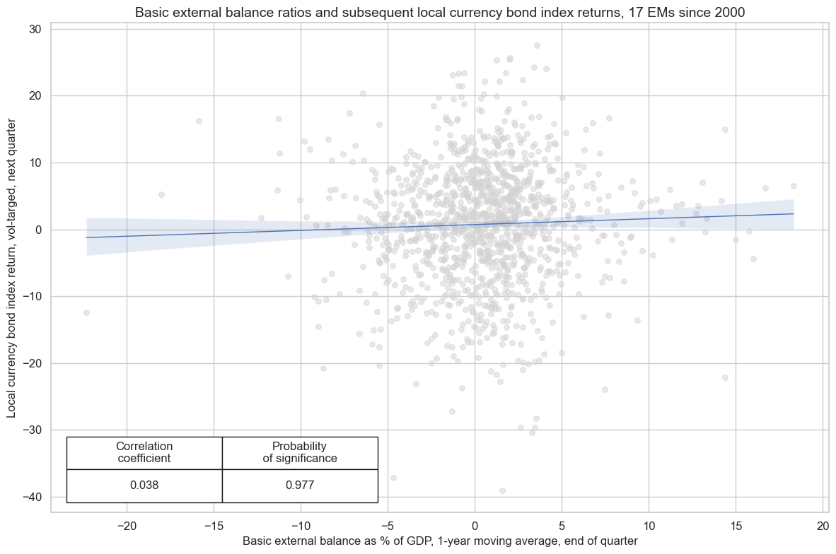
External surpluses often add to appreciation pressure or central bank interventions with related local liquidity supply. Hence, there should be a positive relation between external surpluses and subsequent local bond returns. Indeed, there are modest signs of positive predictive power of basic external balance ratios for subsequent EM local currency bond (index) returns across countries and intertemporally.
feat = "BXBGDPRATIO_NSA_12MMA"
targ = "LCBIXR_VT10"

cidx = msm.common_cids(dfd, xcats=[feat, targ])
print(f"There are {len(cidx)} common cids: \n {cidx}")
sdate = "2000-01-01"

cr = msp.CategoryRelations(
    dfd,
    xcats=[feat, targ],
    cids=cidx,
    blacklist=fxblack,
    freq="q",
    lag=1,
    xcat_aggs=["last", "sum"],
    start=sdate,
    xcat_trims=[40, 40],
)

cr.reg_scatter(
    title="Basic external balance ratios and subsequent local currency bond index returns, 17 EMs since 2000",
    labels=False,
    coef_box="lower left",
    xlab="Basic external balance as % of GDP, 1-year moving average, end of quarter",
    ylab="Local currency bond index return, vol-targed, next quarter",
    prob_est="map"
)
There are 17 common cids:
 ['BRL', 'CLP', 'CNY', 'COP', 'CZK', 'HUF', 'IDR', 'MXN', 'MYR', 'PEN', 'PHP', 'PLN', 'RON', 'RUB', 'THB', 'TRY', 'ZAR']
The enhanced external balance ratio reveals the statistical significant negative correlation between external balances and CDS returns for EM.
feat = "BXBGDPRATIOE_NSA_12MMA"
targ = "CDS02YXR_VT10"

cidx = cids_em
print(f"There are {len(cidx)} common cids: \n {cidx}")
sdate = "2000-01-01"

cr = msp.CategoryRelations(
    dfd,
    xcats=[feat, targ],
    cids=cidx,
    freq="q",
    lag=1,
    xcat_aggs=["last", "sum"],
    start=sdate,
    xcat_trims=[40, 40],
)

cr.reg_scatter(
    title="Enhanced external balance ratios and subsequent sovereign CDS returns, 17 EMs since 2000",
    labels=False,
    coef_box="lower left",
    xlab="Enhanced external balance as % of GDP, 1-year moving average, end of quarter",
    ylab="Sovereign CDS return, vol-targed, next quarter",
    prob_est="map"
)
There are 22 common cids:
 ['BRL', 'COP', 'CLP', 'MXN', 'PEN', 'CZK', 'HUF', 'ILS', 'PLN', 'RON', 'RUB', 'TRY', 'ZAR', 'CNY', 'IDR', 'INR', 'KRW', 'MYR', 'PHP', 'SGD', 'THB', 'TWD']
CDS02YXR_VT10 misses: ['INR', 'SGD', 'TWD'].
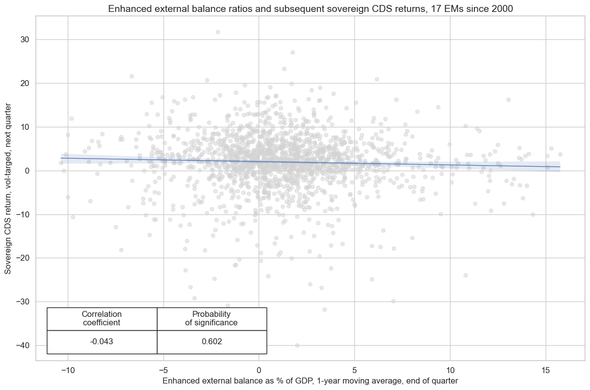
Enhanced external balances or one important aspect of the risk to sovereign credit. Typically countries with high external deficits are more vulnerable to external funding shocks and more prone to sudden currency depreciation, which would reduce a government’s revenue base relative to its foreign-currency debt stock. By itself greater macro risk is ambiguous as a predictor of returns. High deficits indicate high risk but also high premia being paid for those who are invested. However, looking at macro risk in conjunction with priced risk, here in form of spreads, is a legitimate predictor of excess risk premia in the market.
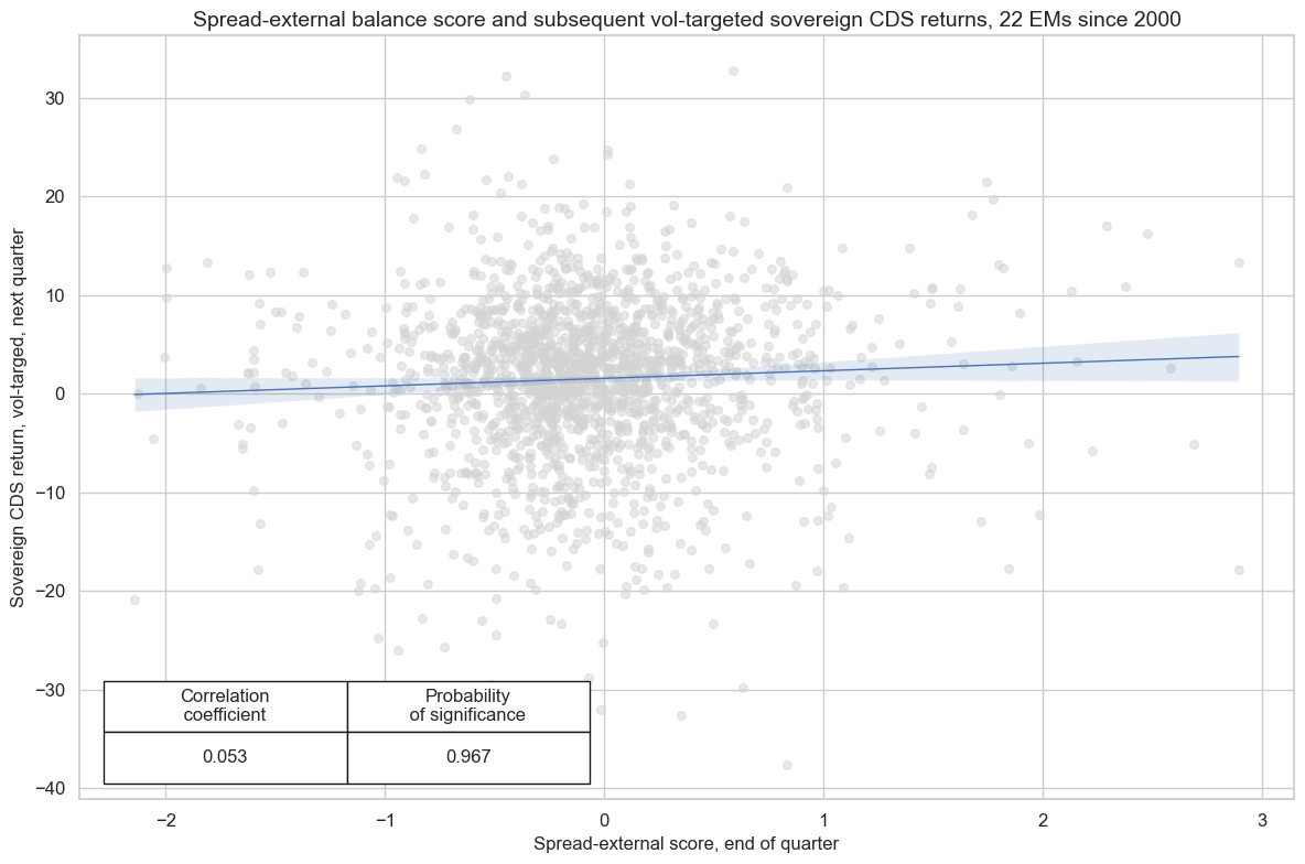
Here we built a spread-external balance score that normalizes spreads and the enhanced basic external balances and then takes the difference between spread scores and external deficit scores. The difference is an unbiased estimate of excess premia. Following it is not just a reach for yield (as would be the spread or deficit score alone) but a legitimate criterion of gaps between market prices and fundamentals.
There has indeed been a significant positive relation between spread-external balance scores and subsequent excess returns, whether vol-targeted or not, at both a monthly and quarterly frequency.
#Creating z-scores for CDS spreads and enhanced external balance
xcatxx = ["BXBGDPRATIOE_NSA_12MMA", "CDS05YSPRD_NSA"]
neutral_dict = {"CDS05YSPRD_NSA": "mean", "BXBGDPRATIOE_NSA_12MMA": "zero"}
cidx = cids_em

for xc in xcatxx:
        dfa = msp.make_zn_scores(
            dfd,
            xcat=xc,
            cids=cidx,
            sequential=True,
            min_obs=261 * 3,
            neutral=neutral_dict[xc],
            pan_weight=1,
            thresh=3,
            postfix="_ZN",
            est_freq="m",
        )
        dfd = msm.update_df(dfd, dfa)
# Calculating the spread-external balance score
cidx = cids_em
xcatx = ["CDS05YSPRD_NSA_ZN", "BXBGDPRATIOE_NSA_12MMA_ZN"]

dfa = msp.linear_composite(
    df=dfd,
    xcats=xcatx,
    signs=[1, 1],
    cids=cidx,
    complete_xcats=False,
    new_xcat="CDS05YSPRD_BXBGDPRATIOE",
)

dfd = msm.update_df(dfd, dfa)
feat = "CDS05YSPRD_BXBGDPRATIOE"
targ = "CDS05YXR_VT10"

cidx = cids_em
print(f"There are {len(cidx)} common cids: \n {cidx}")
sdate = "2000-01-01"

cr = msp.CategoryRelations(
    dfd,
    xcats=[feat, targ],
    cids=cidx,
    freq="q",
    lag=1,
    xcat_aggs=["last", "sum"],
    start=sdate,
    xcat_trims=[40, 40],  # removes single outlier
)

cr.reg_scatter(
    title="Spread-external balance score and subsequent vol-targeted sovereign CDS returns, 22 EMs since 2000",
    labels=False,
    coef_box="lower left",
    xlab="Spread-external score, end of quarter",
    ylab="Sovereign CDS return, vol-targed, next quarter",
    prob_est="map"
)
There are 22 common cids:
 ['BRL', 'COP', 'CLP', 'MXN', 'PEN', 'CZK', 'HUF', 'ILS', 'PLN', 'RON', 'RUB', 'TRY', 'ZAR', 'CNY', 'IDR', 'INR', 'KRW', 'MYR', 'PHP', 'SGD', 'THB', 'TWD']
CDS05YXR_VT10 misses: ['INR', 'SGD', 'TWD'].
Appendices #
Appendix 1: Seasonal adjustment procedure #
We deploy the state-of-the-art US Census X-13 algorithm to handle seasonality in economic series. There are two characteristics of the model worth noting in connection to the point-in-time estimation JPMaQS is delivering:
-
The underlying econometric model is a seasonal ARIMA model leveraging a two-sided filter. As both the earliest and latest observations are included in the historical seasonal component estimation, JPMaQS forces the model (and seasonal component) to being re-estimated for each release date’s time-series. This ensures that only information available at a given point-in-time is used, avoiding leakage of future information.
-
The algorithm has an embedded endogenous model specification using an Akaike Information Criteria, ensuring the parameters are dynamically chosen using only information available at each point-in-time.
For our seasonally adjustment of the Merchandise Trade Balances , we sequentially apply the multiplicative method of the U.S. Census X-13 algorithm to the levels of imports and exports respectively for each of their vintages. We then subtract the imports from the exports to get the seasonally adjusted merchandise trade balances, and take ratios to nominal GDP at the end. This contrast with the Current Account Balances , were we first take the ratio to GDP to deal deal with non-stationarity in the data, and then apply the additive X-13 method to these ratios for each release date. As current account balances can be both in surplus and deficit, we cannot use the multiplicative method to deal with the non-stationarity of the data.
Appendix 2: Notes on OECD data integration #
Some indicators in this notebook are constructed using vintages provided by the OECD’s Revision Analysis Dataset in addition to national sources series’. The integration of the OECD datasets follows the following rules:
-
The following priority order is applied for combining vintages. First, JPMaQS uses seasonally and calendar adjusted original vintages from national sources. Beyond that JPMaQS uses OECD vintages.
-
OECD vintages inform on the month of release but not the exact date. Actual release dates for these vintages are estimated based on release days of subsequent vintages.
-
Inconsistencies, data errors and missing values in the OECD vintages have been corrected for JPMaQS.
OECD data is seasonally adjusted and denominated in native currency. No such consistency is found in national sources. Often figures are stated in a foreign denomination (EUR or USD) and no seasonal adjustment has been applied. To integrate these two data sources we first currency convert national sources into their native currency and then apply seasonal adjustment.
Appendix 3: Currency symbols #
The word ‘cross-section’ refers to currencies, currency areas or economic areas. In alphabetical order, these are AED (Emirates dirham), ARS (Argentine Peso), AUD (Australian dollar), BRL (Brazilian real), CAD (Canadian dollar), CHF (Swiss franc), CLP (Chilean peso), CNY (Chinese yuan renminbi), COP (Colombian peso), CZK (Czech Republic koruna), DEM (German mark), DOP (Dominican Peso), EGP (Egyptian Pound), ESP (Spanish peseta), EUR (Euro), FRF (French franc), GBP (British pound), HKD (Hong Kong dollar), HUF (Hungarian forint), IDR (Indonesian rupiah), ITL (Italian lira), JPY (Japanese yen), KRW (Korean won), MXN (Mexican peso), MYR (Malaysian ringgit), NGN (Nigerian Naira), NLG (Dutch guilder), NOK (Norwegian krone), NZD (New Zealand dollar), OMR (Omani Rial), PAB (Panamanian balboa), PEN (Peruvian sol), PHP (Phillipine peso), PLN (Polish zloty), QAR (Qatari riyal), RON (Romanian leu), RSD (Serbian Dinar), RUB (Russian ruble), SAR (Saudi riyal), SEK (Swedish krona), SGD (Singaporean dollar), THB (Thai baht), TRY (Turkish lira), TWD (Taiwanese dollar), USD (U.S. dollar), UYU (Uruguayan peso), VEF (Venezuelan bolívar), ZAR (South African rand).
Appendix 4: Stable flows in net errors and omissions (NEO) #
As described by Collin, M. (2019) : “One of the most common ways of estimating illicit flows relies on methods developed in the capital flight literature. Researchers often use macroeconomic identities, specifically balance-of-payment statistics, to determine when capital is shifting overseas. […] The “hot-money-narrow method” focuses only on the net errors and omissions (NEOs) entry in balance-of-payment statistics, and occasionally also on flows of short-term capital. The underlying argument is that because NEOs are unexplained, they are more likely to capture hidden flows.”
Based on the “Hot-Money-Narrow” method, we identify stable flows of net errors and omissions (NEO) and incorporate their value into the basic external balance calculation. Since legitimate errors and omissions should, in principle, be equally likely to be positive or negative, we classify NEO flows as stable if they have remained consistently positive or negative for at least 18 out of the past 24 months. When this criterion is met, NEO flows are included in the enhanced external balance calculation.