Government debt ownership #
This category group contains point-in-time information states of central government debt ownership shares by domestic and foreign institutional investors. The data is sourced from a variety of national and international organisations.
Imports #
Only the standard Python data science packages and the specialized
macrosynergy
package are needed.
import os
import pandas as pd

import macrosynergy.management as msm
import macrosynergy.panel as msp
import macrosynergy.visuals as msv

from macrosynergy.download import JPMaQSDownload

from timeit import default_timer as timer
from datetime import timedelta, date

import warnings

warnings.simplefilter("ignore")
The
JPMaQS
indicators we consider are downloaded using the J.P. Morgan Dataquery API interface within the
macrosynergy
package. This is done by specifying
ticker strings
, formed by appending an indicator category code
<category>
to a currency area code
<cross_section>
. These constitute the main part of a full quantamental indicator ticker, taking the form
DB(JPMAQS,<cross_section>_<category>,<info>)
, where
<info>
denotes the time series of information for the given cross-section and category.
The following types of information are available:
-
valuegiving the latest available values for the indicator -
eop_lagreferring to days elapsed since the end of the observation period -
mop_lagreferring to the number of days elapsed since the mean observation period -
gradedenoting a grade of the observation, giving a metric of real time information quality.
After instantiating the
JPMaQSDownload
class within the
macrosynergy.download
module, one can use the
            download(tickers,


            start_date,


            metrics)
method to obtain the data. Here
tickers
is an array of ticker strings,
start_date
is the first release date to be considered and
metrics
denotes the types of information requested.
# Cross-sections of interest
debt_cids = sorted([
    "GBP", "JPY", "USD", "DEM", "FRF", "ITL", "ESP", "NLG", "AUD", "CAD", "CHF", "NZD", "SEK",

])
support_cids = ["EUR"]  # for Duration indicators

cids = debt_cids + support_cids
# Quantamental categories of interest
main = [
    f"{c}{at}"
    for c in [
        "CGCBHDSRATIO",
        "CGFOHDSRATIO",
        "CGPIHDSRATIO",
        "CGFREEFLOATDSRATIO",
        "CGCBHDSGDPRATIO",
        "CGFOHDSGDPRATIO",
        "CGPIHDSGDPRATIO",
        "CGFREEFLOATDSGDPRATIO",
    ]
    for at in [
        "_NSA",
        "_NSA_3MMA",
        "_NSA_D1M1ML1",
        "_NSA_D3M3ML3",
        "_NSA_D1M1ML12",
        "_NSA_3MMA_D1M1ML12",
    ]
]

econ = [
    # Monetary base level and growth (real)
    "MBASEGDP_SA_D1M1ML3",

    "RMBROAD_SJA_P1M1ML12",
    "RMNARROW_SJA_P1M1ML12",

    "RMBROAD_SJA_P3M3ML3AR",
    "RMNARROW_SJA_P3M3ML3AR",

    # Intervention liquidity
    "INTLIQGDP_NSA_D1M1ML3",

    # Duration Carry
    "DU02YCRY_NSA",
    "DU05YCRY_NSA",
    "DU02YCRY_VT10",
    "DU05YCRY_VT10",

    # Government bond carry
    "GB02YCRY_NSA",
    "GB05YCRY_NSA",
    "GB02YCRY_VT10",
    "GB05YCRY_VT10",

    # Government bond yields - real
    "GB02YRYLD_VT10",
    "GB05YRYLD_VT10"
]  # economic context

mark = [
    # Duration returns
    "DU02YXR_NSA",
    "DU05YXR_NSA",
    "DU10YXR_NSA",
    "DU02YXR_VT10",
    "DU05YXR_VT10",
    "DU10YXR_VT10",
    # Government bonds
    "GB02YXR_NSA",
    "GB05YXR_NSA",
    "GB10YXR_NSA",
    "GB02YXR_VT10",
    "GB05YXR_VT10",
    "GB10YXR_VT10",
]  # market links

xcats = main + econ + mark
# Download series from J.P. Morgan DataQuery by tickers

start_date = "2000-01-01"
tickers = [cid + "_" + xcat for cid in cids for xcat in xcats]
print(f"Maximum number of tickers is {len(tickers)}")

# Retrieve credentials

client_id: str = os.getenv("DQ_CLIENT_ID")
client_secret: str = os.getenv("DQ_CLIENT_SECRET")

# Download from DataQuery

with JPMaQSDownload(client_id=client_id, client_secret=client_secret) as downloader:
    start = timer()
    df = downloader.download(
        tickers=tickers,
        start_date=start_date,
        metrics=["value", "eop_lag", "mop_lag", "grading"],
        suppress_warning=True,
        show_progress=True,
    )
    end = timer()

dfd = df

print("Download time from DQ: " + str(timedelta(seconds=end - start)))
Maximum number of tickers is 1064
Downloading data from JPMaQS.
Timestamp UTC:  2025-04-29 16:20:16
Connection successful!
Requesting data: 100%|███████████████████████████████████████████████████████████████| 213/213 [00:47<00:00,  4.47it/s]
Downloading data: 100%|██████████████████████████████████████████████████████████████| 213/213 [01:10<00:00,  3.01it/s]
Some expressions are missing from the downloaded data. Check logger output for complete list.
800 out of 4256 expressions are missing. To download the catalogue of all available expressions and filter the unavailable expressions, set `get_catalogue=True` in the call to `JPMaQSDownload.download()`.
Some dates are missing from the downloaded data.
2 out of 6609 dates are missing.
Download time from DQ: 0:02:10.487885
Availability #
cids_exp = debt_cids  # cids expected in category panels
msm.missing_in_df(dfd, xcats=main, cids=cids_exp)
No missing XCATs across DataFrame.
Missing cids for CGCBHDSGDPRATIO_NSA:                      []
Missing cids for CGCBHDSGDPRATIO_NSA_3MMA:                 []
Missing cids for CGCBHDSGDPRATIO_NSA_3MMA_D1M1ML12:        []
Missing cids for CGCBHDSGDPRATIO_NSA_D1M1ML1:              []
Missing cids for CGCBHDSGDPRATIO_NSA_D1M1ML12:             []
Missing cids for CGCBHDSGDPRATIO_NSA_D3M3ML3:              []
Missing cids for CGCBHDSRATIO_NSA:                         []
Missing cids for CGCBHDSRATIO_NSA_3MMA:                    []
Missing cids for CGCBHDSRATIO_NSA_3MMA_D1M1ML12:           []
Missing cids for CGCBHDSRATIO_NSA_D1M1ML1:                 []
Missing cids for CGCBHDSRATIO_NSA_D1M1ML12:                []
Missing cids for CGCBHDSRATIO_NSA_D3M3ML3:                 []
Missing cids for CGFOHDSGDPRATIO_NSA:                      []
Missing cids for CGFOHDSGDPRATIO_NSA_3MMA:                 []
Missing cids for CGFOHDSGDPRATIO_NSA_3MMA_D1M1ML12:        []
Missing cids for CGFOHDSGDPRATIO_NSA_D1M1ML1:              []
Missing cids for CGFOHDSGDPRATIO_NSA_D1M1ML12:             []
Missing cids for CGFOHDSGDPRATIO_NSA_D3M3ML3:              []
Missing cids for CGFOHDSRATIO_NSA:                         []
Missing cids for CGFOHDSRATIO_NSA_3MMA:                    []
Missing cids for CGFOHDSRATIO_NSA_3MMA_D1M1ML12:           []
Missing cids for CGFOHDSRATIO_NSA_D1M1ML1:                 []
Missing cids for CGFOHDSRATIO_NSA_D1M1ML12:                []
Missing cids for CGFOHDSRATIO_NSA_D3M3ML3:                 []
Missing cids for CGFREEFLOATDSGDPRATIO_NSA:                []
Missing cids for CGFREEFLOATDSGDPRATIO_NSA_3MMA:           []
Missing cids for CGFREEFLOATDSGDPRATIO_NSA_3MMA_D1M1ML12:  []
Missing cids for CGFREEFLOATDSGDPRATIO_NSA_D1M1ML1:        []
Missing cids for CGFREEFLOATDSGDPRATIO_NSA_D1M1ML12:       []
Missing cids for CGFREEFLOATDSGDPRATIO_NSA_D3M3ML3:        []
Missing cids for CGFREEFLOATDSRATIO_NSA:                   []
Missing cids for CGFREEFLOATDSRATIO_NSA_3MMA:              []
Missing cids for CGFREEFLOATDSRATIO_NSA_3MMA_D1M1ML12:     []
Missing cids for CGFREEFLOATDSRATIO_NSA_D1M1ML1:           []
Missing cids for CGFREEFLOATDSRATIO_NSA_D1M1ML12:          []
Missing cids for CGFREEFLOATDSRATIO_NSA_D3M3ML3:           []
Missing cids for CGPIHDSGDPRATIO_NSA:                      ['CHF']
Missing cids for CGPIHDSGDPRATIO_NSA_3MMA:                 ['CHF']
Missing cids for CGPIHDSGDPRATIO_NSA_3MMA_D1M1ML12:        ['CHF']
Missing cids for CGPIHDSGDPRATIO_NSA_D1M1ML1:              ['CHF']
Missing cids for CGPIHDSGDPRATIO_NSA_D1M1ML12:             ['CHF']
Missing cids for CGPIHDSGDPRATIO_NSA_D3M3ML3:              ['CHF']
Missing cids for CGPIHDSRATIO_NSA:                         ['CHF']
Missing cids for CGPIHDSRATIO_NSA_3MMA:                    ['CHF']
Missing cids for CGPIHDSRATIO_NSA_3MMA_D1M1ML12:           ['CHF']
Missing cids for CGPIHDSRATIO_NSA_D1M1ML1:                 ['CHF']
Missing cids for CGPIHDSRATIO_NSA_D1M1ML12:                ['CHF']
Missing cids for CGPIHDSRATIO_NSA_D3M3ML3:                 ['CHF']
For the explanation of currency symbols, which are related to currency areas or countries for which categories are available, please view Appendix 1 .
xcatx = [xc for xc in main if xc.endswith("_NSA")]
cidx = debt_cids

dfx = msm.reduce_df(dfd, xcats=xcatx, cids=cidx)
dfs = msm.check_startyears(
    dfx,
)
msm.visual_paneldates(dfs, size=(20, 6))

print("Last updated:", date.today())
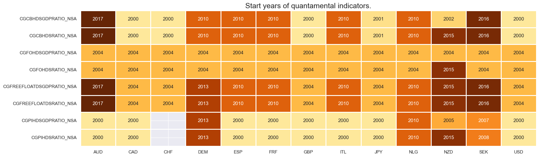
Last updated: 2025-04-29
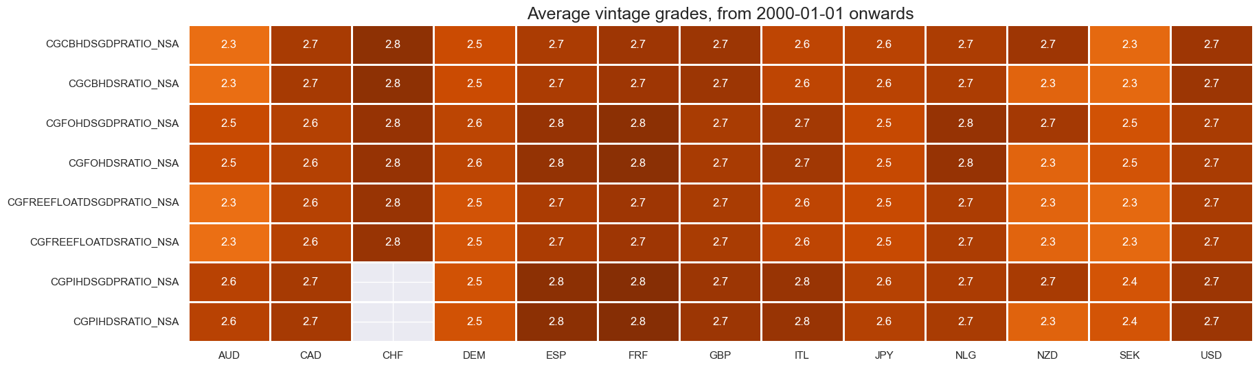
Average grades are on the low side at the moment, as electronic vintage records are not yet easily available. This, in turn, reflects that these surveys are not as carefully watched as other indicator.
xcatx = [xc for xc in main if xc.endswith("_NSA")]
cidx = debt_cids

plot = msp.heatmap_grades(
    dfd,
    xcats=xcatx,
    cids=cidx,
    start=start_date,
    size=(20, 6),
    title=f"Average vintage grades, from {start_date} onwards",
)
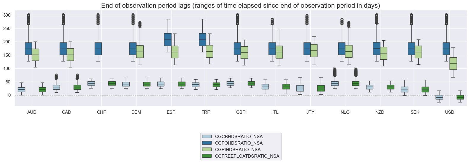
Timeliness of reporting versus the declared observation period is quite different across countries. This may partly reflect different labeling conventions, however.
USD central bank holdings ratio and, as a consequence, free-float ratios are updated at weekly frequency: this is the reason behind these indicators’ negative value for end-of-period lag.
xcatx = [
    "CGCBHDSRATIO_NSA",
    "CGFOHDSRATIO_NSA",
    "CGPIHDSRATIO_NSA",
    "CGFREEFLOATDSRATIO_NSA",
]
cidx = debt_cids

msp.view_ranges(
    dfd,
    xcats=xcatx,
    cids=cidx,
    val="eop_lag",
    title="End of observation period lags (ranges of time elapsed since end of observation period in days)",
    start="2000-01-01",
    kind="box",
    size=(16, 6),
)
History #
Security holdings as shares of outstanding #
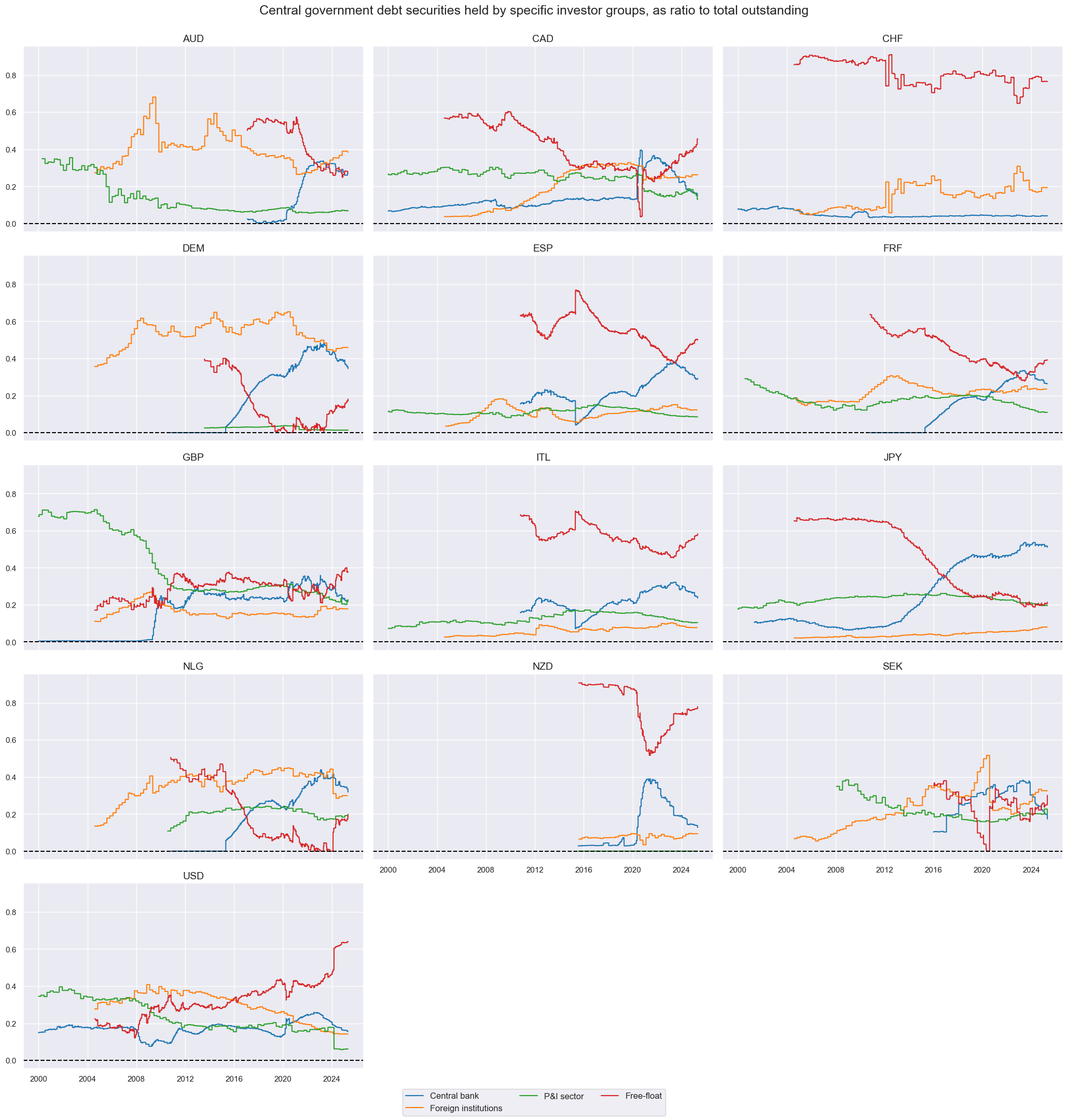
The shares of free-floating government securities are vastly different across countries. Also, medium-term dynamics have been quite different.
xcatx = [
    "CGCBHDSRATIO_NSA",
    "CGFOHDSRATIO_NSA",
    "CGPIHDSRATIO_NSA",
    "CGFREEFLOATDSRATIO_NSA",
]

msp.view_timelines(
    dfd,
    xcats=xcatx,
    cids=debt_cids,
    start=start_date,
    title="Central government debt securities held by specific investor groups, as ratio to total outstanding",
    xcat_labels=[
        "Central bank",
        "Foreign institutions",
        "P&I sector",
        "Free-float"
    ],
    ncol=3,
    same_y=True,
    all_xticks=False,
)
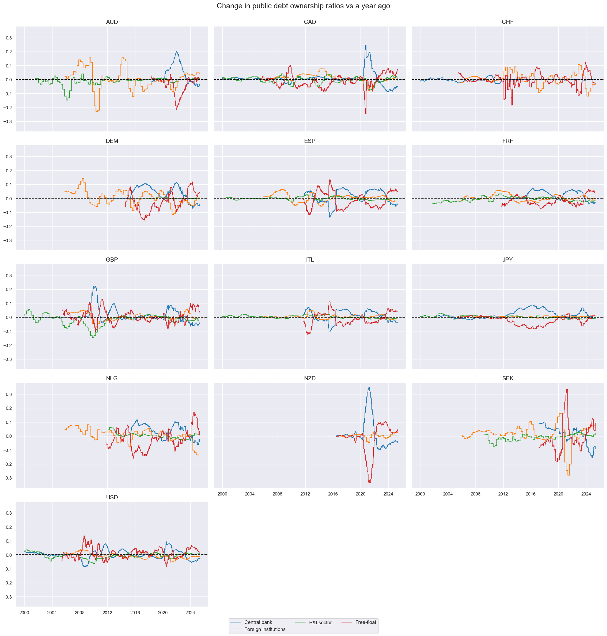
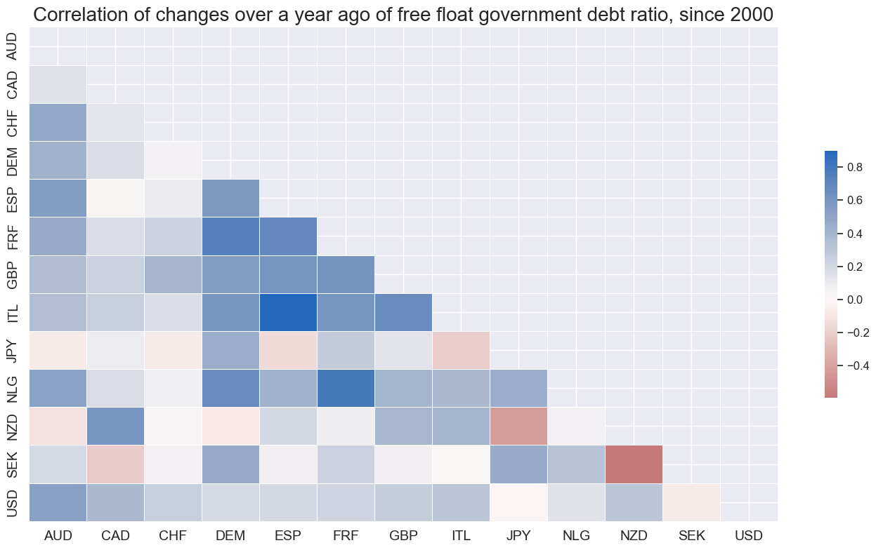
Changes in government securities holding shares #
Changes in free-floating government securities shares have been positively correlated over the past two decades, reflecting similar monetary policies across countries.
xcatx = [
    "CGCBHDSRATIO_NSA_3MMA_D1M1ML12",
    "CGFOHDSRATIO_NSA_3MMA_D1M1ML12",
    "CGPIHDSRATIO_NSA_3MMA_D1M1ML12",
    "CGFREEFLOATDSRATIO_NSA_3MMA_D1M1ML12",
]
cidx = debt_cids

msp.view_timelines(
    dfd,
    xcats=xcatx,
    cids=cidx,
    start=start_date,
    title="Change in public debt ownership ratios vs a year ago",
    ncol=3,
    same_y=True,
    all_xticks=False,
    xcat_labels=[
        "Central bank",
        "Foreign institutions",
        "P&I sector",
        "Free-float"
    ]
)
msp.correl_matrix(
    dfd,
    xcats="CGFREEFLOATDSRATIO_NSA_3MMA_D1M1ML12",
    cids=debt_cids,
    start=start_date,
    title="Correlation of changes over a year ago of free float government debt ratio, since 2000",
)
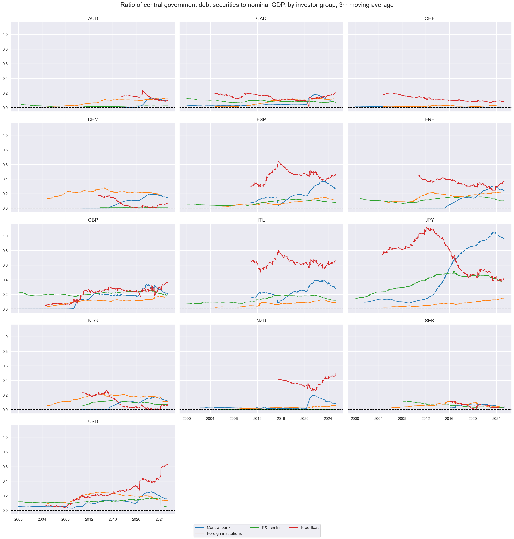
Ratios to nominal GDP #
Differences in free-floating debt securities ratios reflect largely differences in outstanding government debt. The relative dynamics of the U.S. (medium-term increase) and Japan (medium-term decrease) have been striking.
xcatx = [
    "CGCBHDSGDPRATIO_NSA_3MMA",
    "CGFOHDSGDPRATIO_NSA_3MMA",
    "CGPIHDSGDPRATIO_NSA_3MMA",
    "CGFREEFLOATDSGDPRATIO_NSA_3MMA",
]

msp.view_timelines(
    dfd,
    xcats=xcatx,
    cids=debt_cids,
    start=start_date,
    title="Ratio of central government debt securities to nominal GDP, by investor group, 3m moving average",
    xcat_labels=[
        "Central bank",
        "Foreign institutions",
        "P&I sector",
        "Free-float"
    ],
    ncol=3,
    same_y=True,
    all_xticks=False,
)
Importance #
Research links #
“Domestic financial institutions allocated a larger share of government securities in their portfolios, as Japan has done since its crisis in the 1990s. Increases in the share held by institutional investors or non-residents by 10 percentage points are associated with a reduction in yields by about 25 or 40 basis points, respectively.” IMF 2012
“The paper proposes a framework—sovereign funding shock scenarios (FSS)—to conduct forward-looking analysis to assess sovereigns’ vulnerability to sudden investor outflows, which can be used along with standard debt sustainability analyses (DSA). It also introduces two risk indices—investor base risk index (IRI) and foreign investor position index (FIPI)—to assess sovereigns’ vulnerability to shifts in investor behavior.” IMF 2012a
“Institutions exhibit substantial heterogeneity in trading behavior. Although many studies consider their investment horizon or portfolio concentration in isolation, we propose a two-way investor classification that jointly accounts for both characteristics. Our conceptual framework provides an intuitive account of each institutional investor group’s trading and the ensuing impact on market price dynamics, offering fresh insights into seemingly mixed findings in the literature. Our results indicate that a short investment horizon and a high portfolio concentration are both proxies for an informational advantage.” Kim et al. 2021
Empirical clues #
Data preparation #
We are interested in relating various aspects of macroeconomic balance sheets with asset returns for the majority of the countries where financial instruments are available.
In order to do this, we associate JPMaQS quantamental indicators available for the aggregate Euro area to each of the single European countries. This includes various measures of interest rate swap returns and carry.
dfx = df.copy(deep=True)
eur_df = dfx.loc[(dfx["cid"] == "EUR") & (dfx["xcat"].isin([
    "DU02YXR_NSA",
    "DU05YXR_NSA",
    "DU10YXR_NSA",
    "DU02YXR_VT10",
    "DU05YXR_VT10",
    "DU10YXR_VT10",
    "DU02YCRY_NSA",
    "DU05YCRY_NSA",
    "DU02YCRY_VT10",
    "DU05YCRY_VT10",
    "MBASEGDP_SA_D1M1ML3",
    "RMBROAD_SJA_P1M1ML12",
    "RMNARROW_SJA_P1M1ML12",
    "RMBROAD_SJA_P3M3ML3AR",
    "RMNARROW_SJA_P3M3ML3AR",
    "INTLIQGDP_NSA_D1M1ML3",
]))]

dfx = pd.concat([dfx] + [
    eur_df.drop(columns="cid").assign(cid=cc) for cc in ["DEM", "FRF", "ITL", "NLG", "ESP"]
], ignore_index=True, axis=0)

dfx = dfx.sort_values(by=["cid", "xcat", "real_date"])
Sovereign debt ownership changes and asset swap returns #
We compute returns for an asset swap position across all countries where both government bond and IRS returns are available. The asset swap buyer is long a bond and hedges the interest rate (duration) risk by paying fixed and receiving floating in an interest rate swap
By virtue of calculation methodology of JPMaQS duration returns and generic government bond returns , the asset swap spread reflects sovereign credit risk, liquidity risk, repurchase agreement conditions, supply and demand imbalances, and clearing house collateral standards.
cidx = debt_cids

calcs = [
    f"ASSETSWAP{tenor}YXR_{adj} = GB{tenor}YXR_{adj} - DU{tenor}YXR_{adj}"
    for tenor in ["02", "05", "10"]
    for adj in ["NSA", "VT10"]
]

dfa = msp.panel_calculator(dfx, calcs=calcs, cids=cidx)
dfx = msm.update_df(dfx, dfa)
xcatx = [
    f"ASSETSWAP{tenor}YXR_{adj}" for tenor in ["02", "05", "10"] for adj in ["NSA", "VT10"]
]
cidx = debt_cids

msm.missing_in_df(dfx, xcats=xcatx, cids=cidx)
No missing XCATs across DataFrame.
Missing cids for ASSETSWAP02YXR_NSA:   ['CAD', 'CHF', 'NLG', 'SEK']
Missing cids for ASSETSWAP02YXR_VT10:  ['CAD', 'CHF', 'NLG', 'SEK']
Missing cids for ASSETSWAP05YXR_NSA:   ['CAD', 'CHF', 'NLG', 'SEK']
Missing cids for ASSETSWAP05YXR_VT10:  ['CAD', 'CHF', 'NLG', 'SEK']
Missing cids for ASSETSWAP10YXR_NSA:   ['CAD', 'CHF', 'NLG', 'SEK']
Missing cids for ASSETSWAP10YXR_VT10:  ['CAD', 'CHF', 'NLG', 'SEK']
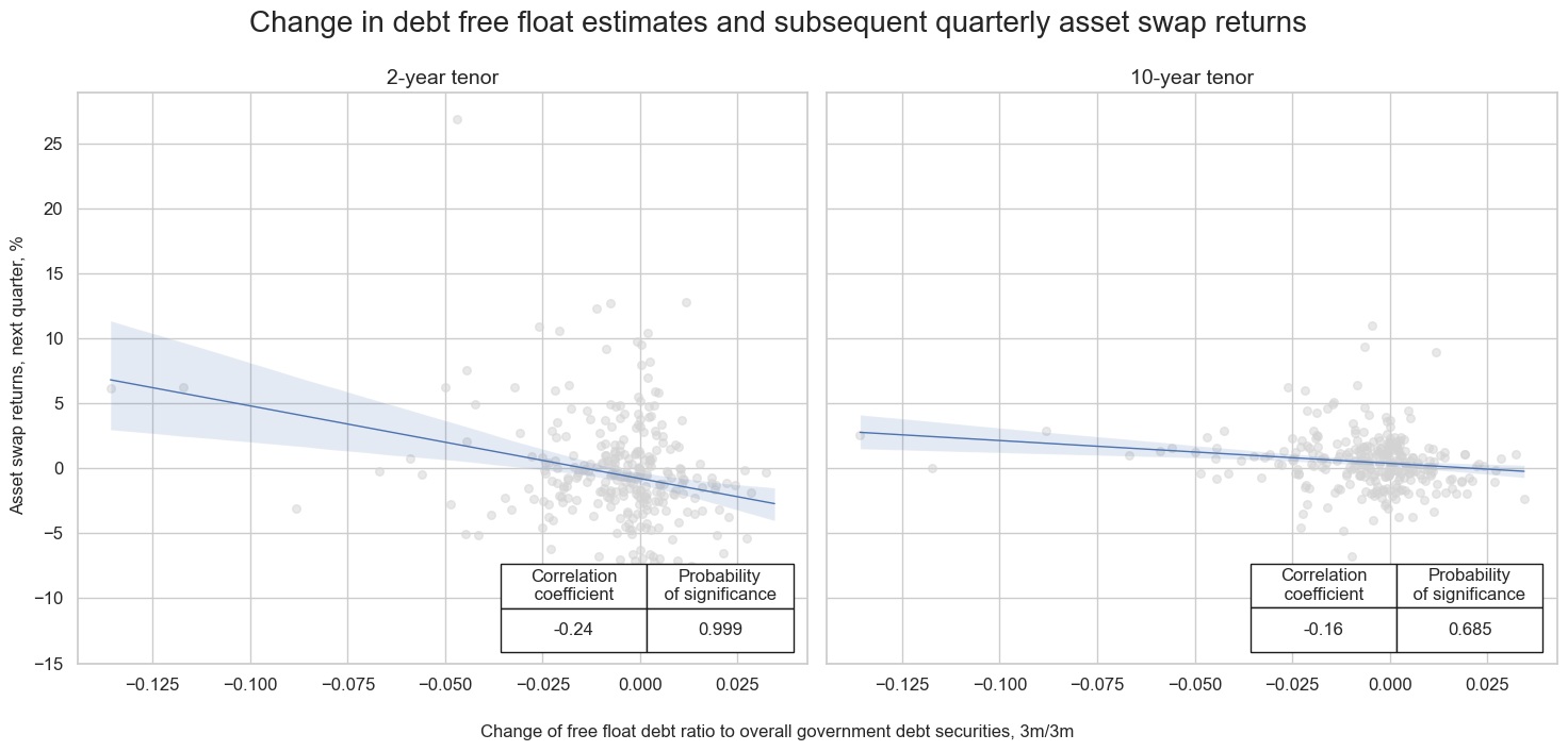
Plausibly a reduction in government debt securities available to the broad market should, by itself, reduce swap spreads, as it reduces the specific supply of the asset.
Empirically, a reduction in free-floating government securities’ share of total securities or of GDP has negatively predicted asset swap returns. At shorter-maturities the relation is highly significant.
cidx = ["AUD", "DEM", "GBP", "JPY", "NZD", "USD"] # only the relevant cross-sections
sdate = "2010-01-01"


qcr_2y10yas = {
   target_cat: msp.CategoryRelations(
    dfx,
    xcats=["CGFREEFLOATDSRATIO_NSA_D3M3ML3", target_cat],
    cids=cidx,
    freq="Q",
    start=sdate,
    lag=1,
    slip=1,
    years=None,
    xcat_aggs=["last", "sum"]
   )
   for target_cat in ["ASSETSWAP02YXR_VT10", "ASSETSWAP10YXR_VT10"]
}

msv.multiple_reg_scatter(
    cat_rels=list(qcr_2y10yas.values()),
    ncol=2, nrow=1,
    figsize=(15, 7),
    title='Change in debt free float estimates and subsequent quarterly asset swap returns',
    xlab='Change of free float debt ratio to overall government debt securities, 3m/3m',
    ylab='Asset swap returns, next quarter, %',
    fit_reg=True,
    coef_box="lower right",
    coef_box_size=(0.4, 2.5),
    prob_est='map',
    separator=None,
    single_chart=False,
    subplot_titles=[
       "2-year tenor", "10-year tenor"
    ],
)
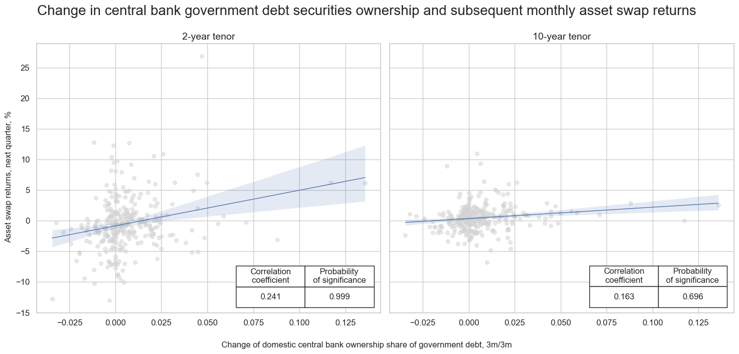
The central banks’ actions seem to have strongest predictive power, partly because in past decades quantitative and qualitative easing has been a major policy and partly because information of their actions is available with only short publication delays.
cidx = ["AUD", "DEM", "GBP", "JPY", "NZD", "USD"] # only the relevant cross-sections
sdate = "2010-01-01"


qcr_cb2y10yas = {
   target_cat: msp.CategoryRelations(
    dfx,
    xcats=["CGCBHDSRATIO_NSA_D3M3ML3", target_cat],
    cids=cidx,
    freq="Q",
    start=sdate,
    lag=1,
    slip=1,
    years=None,
    xcat_aggs=["last", "sum"]
   )
   for target_cat in ["ASSETSWAP02YXR_VT10", "ASSETSWAP10YXR_VT10"]
}

msv.multiple_reg_scatter(
    cat_rels=list(qcr_cb2y10yas.values()),
    ncol=2, nrow=1,
    figsize=(15, 7),
    title='Change in central bank government debt securities ownership and subsequent monthly asset swap returns',
    xlab='Change of domestic central bank ownership share of government debt, 3m/3m',
    ylab='Asset swap returns, next quarter, %',
    fit_reg=True,
    coef_box="lower right",
    coef_box_size=(0.4, 2.5),
    prob_est='map',
    separator=None,
    single_chart=False,
    subplot_titles=[
        "2-year tenor", "10-year tenor"
    ],
)
Appendices #
Appendix 1: Currency symbols #
The word ‘cross-section’ refers to currencies, currency areas or economic areas. In alphabetical order, these are AUD (Australian dollar), BRL (Brazilian real), CAD (Canadian dollar), CHF (Swiss franc), CLP (Chilean peso), CNY (Chinese yuan renminbi), COP (Colombian peso), CZK (Czech Republic koruna), DEM (German mark), ESP (Spanish peseta), EUR (Euro), FRF (French franc), GBP (British pound), HKD (Hong Kong dollar), HUF (Hungarian forint), IDR (Indonesian rupiah), ITL (Italian lira), JPY (Japanese yen), KRW (Korean won), MXN (Mexican peso), MYR (Malaysian ringgit), NLG (Dutch guilder), NOK (Norwegian krone), NZD (New Zealand dollar), PEN (Peruvian sol), PHP (Phillipine peso), PLN (Polish zloty), RON (Romanian leu), RUB (Russian ruble), SEK (Swedish krona), SGD (Singaporean dollar), THB (Thai baht), TRY (Turkish lira), TWD (Taiwanese dollar), USD (U.S. dollar), ZAR (South African rand).