Private consumption

This category group contains information states of trends and conditions related to private consumption. At present this includes real-time standardized and seasonally adjusted measures of private consumption, consumer confidence and retail sales growth. Survey vintages are standardized by using historical means and standard deviations on the survey level. The purpose of standardization based on expanding samples is to replicate the market’s information on what was considered normal in terms of level and deviation and to make metrics more intuitive and comparable across countries.

Private consumption growth

Ticker : RPCONS_SA_P1Q1QL4 / _P1M1ML12 / _P1M1ML12_3MMA

Label : Real Private consumption, sa: % oya (q) / % oya / % oya, 3mma

Definition : Real Private consumption, seasonally adjusted: percentage over a year ago (quarterly) / percentage over a year ago / percentage over a year ago, 3-month moving average

Notes :

• The underlying data is sourced from national accounts. Most countries release quarterly data except for USA (USD) which produces a separate monthly-frequency data.

• China (CNY) does not produce quarterly private consumption data

Private consumption trends

Ticker : RPCONS_SA_P1Q1QL1AR / _P2Q2QL2AR / _P3M3ML3AR / _P6M6ML6AR

Label : Real Private consumption, sa: % 1q/1q ar / % 2q/2q ar / % 3m/3m ar / % 6m/6m ar

Definition : Real Private consumption, seasonally adjusted: % of latest quarter over previous quarter at annualized rate / % of latest 2 quarters over previous 2 quarters at an annualized rate / % of latest 3 months over previous 3 months at annualized rate / % of latest 6 months over previous 6 months at an annualized rate

Notes :

• See notes for private consumption growth

Consumer confidence scores

Ticker : CCSCORE_SA / _3MMA

Label : Consumer confidence, sa: z-score / z-score, 3mma

Definition : Consumer confidence, seasonally adjusted: z-score / z-score, 3-month moving average

Notes :

• The underlying data is sourced from national statistical offices and business groups. Most countries release monthly-frequency data. The exceptions are the following currency areas which produce quarterly data: Switzerland(CHF), New Zealand (NZD), the Phillipines (PHP), Russia (RUB) and South Africa (ZAR).

• Confidence levels are seasonally adjusted, either at the source or by JPMaQS, on a rolling and out-of-sample basis.

• Peru (PEN), Romania (RON) and Singapore (SGD) do not release publicly available consumer surveys, hence they are excluded from this set.

• For in-depth explanation of how the z-scores are computed, please read Appendix 2 .

Consumer confidence scores trends

Ticker : CCSCORE_SA_D1M1ML1 / _D3M3ML3 / _D1Q1QL1 / _D6M6ML6 / _D2Q2QL2 / _D1M1ML12 / _3MMA_D1M1ML12 / _D1Q1QL4

Label : Consumer confidence, sa, z-score: diff m/m / diff 3m/3m / diff q/q / diff 6m/6m / diff 2q/2q / diff oya (m) / diff oya, 3mma / diff oya (q)

Definition : Consumer confidence, seasonally adjusted, z-score: difference over 1 month / difference of last 3 months over previous 3 months / difference of last quarter over previous quarter / difference of last 6 months over previous 6 months / difference of last 2 quarters over previous 2 quarters / difference over a year ago, monthly values / difference over a year ago, 3-month moving average / difference over a year ago, quarterly values

Notes :

• See notes for consumer confidence scores

Retail sales growth

Ticker : NRSALES_SA_P1M1ML12 / _P1M1ML12_3MMA / _P1Q1QL4

Label : Nominal retail sales, sa: % oya / % oya, 3mma / % oya (q)

Definition : Nominal retail sales, seasonally adjusted: percentage over a year ago / percentage over a year ago, 3-month moving average / percentage over a year ago (quarterly)

Notes :

• Chile (CLP), Indonesia (IDR), Isreal (ILS), Mexico (MXN), Malaysia (MYR), Romania (RON), Singpore (SGD) and Taiwan (TWD) only produce real retail sales information and they are not part of this category set.

• Australia (AUD), New Zealand (NZD) and Philippines (PHP) only produce quarterly data.

Ticker : RRSALES_SA_P1M1ML12 / _P1M1ML12_3MMA / _P1Q1QL4

Label : Real retail sales, sa: % oya / % oya, 3mma / % oya (q)

Definition : Real retail sales, seasonally adjusted: percentage over a year ago / percentage over a year ago, 3-month moving average / percentage over a year ago (quarterly)

Notes :

• India (IDR) does not produce official retail trade statisitcs for real or nominal data.

• Australia (AUD), New Zealand (NZD) and Philippines (PHP) only produce quarterly data.

• China (CNY), Thailand (THB) and USA (USD) do not produce real retail sales, to calculate this we take the ratio of nominal retail sales and a form of CPI. For Thailand we use headline CPI, for the USA we use goods CPI and for China we use both as the series for Goods CPI only started being produced in 2011.

• Peru (PEN) we also estimate the real retail sales but as the offical nominal series only produces yearly changes, to estimate this we take the yearly change in nominal retail sales and subtract it from the change in headline CPI.

Imports

Only the standard Python data science packages and the specialized macrosynergy package are needed.

import os
import numpy as np
import pandas as pd
import matplotlib.pyplot as plt
import seaborn as sns

import macrosynergy.management as msm
import macrosynergy.panel as msp
import macrosynergy.signal as mss
import macrosynergy.pnl as msn
import macrosynergy.visuals as msv

from macrosynergy.download import JPMaQSDownload

from timeit import default_timer as timer
from datetime import timedelta, date, datetime

import warnings

warnings.simplefilter("ignore")

The JPMaQS indicators we consider are downloaded using the J.P. Morgan Dataquery API interface within the macrosynergy package. This is done by specifying ticker strings, formed by appending an indicator category code to a currency area code <cross_section>. These constitute the main part of a full quantamental indicator ticker, taking the form DB(JPMAQS,<cross_section>_ , ), where denotes the time series of information for the given cross-section and category.

The following types of information are available:

value giving the latest available values for the indicator eop_lag referring to days elapsed since the end of the observation period mop_lag referring to the number of days elapsed since the mean observation period grade denoting a grade of the observation, giving a metric of real time information quality. After instantiating the JPMaQSDownload class within the macrosynergy.download module, one can use the download(tickers, start_date, metrics) method to obtain the data. Here tickers is an array of ticker strings, start_date is the first release date to be considered and metrics denotes the types of information requested.

# Cross-sections of interest

cids_dmca = [
    "AUD",
    "CAD",
    "CHF",
    "EUR",
    "GBP",
    "JPY",
    "NOK",
    "NZD",
    "SEK",
    "USD",
]  # DM currency areas
cids_dmec = ["DEM", "ESP", "FRF", "ITL", "NLG"]  # DM euro area countries
cids_latm = ["BRL", "COP", "CLP", "MXN", "PEN"]  # Latam countries
cids_emea = ["CZK", "HUF", "ILS", "PLN", "RON", "RUB", "TRY", "ZAR"]  # EMEA countries
cids_emas = [
    "CNY",
    "HKD",
    "IDR",
    "INR",
    "KRW",
    "MYR",
    "PHP",
    "SGD",
    # "THB",
    "TWD",
]  # EM Asia countries

cids_dm = cids_dmca + cids_dmec
cids_em = cids_latm + cids_emea + cids_emas

cids = sorted(cids_dm + cids_em)

# FX cross-sections lists (for research purposes)

cids_nofx = ["EUR", "USD", "SGD"] + cids_dmec
cids_fx = list(set(cids) - set(cids_nofx))

cids_dmfx = set(cids_dm).intersection(cids_fx)
cids_emfx = set(cids_em).intersection(cids_fx)

cids_eur = ["CHF", "CZK", "HUF", "NOK", "PLN", "RON", "SEK"]  # trading against EUR
cids_eud = ["GBP", "RUB", "TRY"]  # trading against EUR and USD
cids_usd = list(set(cids_fx) - set(cids_eur + cids_eud))



cids_exp = sorted(list(set(cids) - set(cids_dmec)))  # cids expected in category panels excluding high yield and investment grade returns

# Sectorial equity index returns
cids_dmeq = ['AUD', 'CAD', 'CHF', 'EUR', 'GBP', 'HKD', 'ILS', 'JPY', 'NOK', 'NZD', 'SEK', 'SGD', 'USD']
cids_eueq = ["DEM", "ESP", "FRF", "ITL", "NLG"]


#cids = sorted(cids_dmeq + cids_eueq + cids_aseq + cids_eeeq + cids_laeq)
sector_cids = sorted(cids_dmeq + cids_eueq)

# Quantamental categories of interest

confs = [
    "CCSCORE_SA",
    "CCSCORE_SA_3MMA",
    "CCSCORE_SA_D1M1ML1",
    "CCSCORE_SA_D3M3ML3",
    "CCSCORE_SA_D1Q1QL1",
    "CCSCORE_SA_D6M6ML6",
    "CCSCORE_SA_D2Q2QL2",
    "CCSCORE_SA_3MMA_D1M1ML12",
    "CCSCORE_SA_D1M1ML12",
    "CCSCORE_SA_D1Q1QL4",
]

sales = [
    "NRSALES_SA_P1M1ML12",
    "NRSALES_SA_P1M1ML12_3MMA",
    "NRSALES_SA_P1Q1QL4",
    "RRSALES_SA_P1M1ML12",
    "RRSALES_SA_P1M1ML12_3MMA",
    "RRSALES_SA_P1Q1QL4",

]

rpcons = [
    "RPCONS_SA_P1M1ML12",
    "RPCONS_SA_P1M1ML12_3MMA",
    "RPCONS_SA_P1Q1QL4",
    "RPCONS_SA_P1Q1QL1AR",
    "RPCONS_SA_P2Q2QL2AR",
    "RPCONS_SA_P3M3ML3AR",
    "RPCONS_SA_P6M6M6AR",
]

main = confs + sales + rpcons

econ = ["RGDP_SA_P1Q1QL4", ]  # economic context

mark = [
    "DU02YXR_VT10",
    "DU05YXR_VT10",
    "EQXR_VT10",
    "FXXR_NSA",
    "FXXR_VT10", 
    "FXTARGETED_NSA",
    "FXUNTRADABLE_NSA",
]  # market links


sector_labels = {
    "ALL": "All sectors", 
    "COD": "Cons. discretionary",
    "COS": "Cons. staples",
    "CSR": "Communication services",
    "ENR": "Energy",
    "FIN": "Financials",
    "HLC": "Healthcare",
    "IND": "Industrials",
    "ITE": "Information tech",
    "MAT": "Materials",
    "REL": "Real estate",
    "UTL": "Utilities",
}
sectors = list(sector_labels.keys())
cids_secs = list(sector_labels.keys())[1:]

vt_xrets = ["EQC" + sec + "XR_VT10" for sec in sectors] 
untradable = ['EQC' + sec + 'UNTRADABLE_NSA' for sec in sectors]

eqret = vt_xrets + untradable #+ simple_xrets

xcats = main + mark + econ + eqret

# Download series from J.P. Morgan DataQuery by tickers

start_date = "1990-01-01"

tickers = [cid + "_" + xcat for cid in cids for xcat in xcats] 

print(f"Maximum number of tickers is {len(tickers)}")

# Retrieve credentials

client_id: str = os.getenv("DQ_CLIENT_ID")
client_secret: str = os.getenv("DQ_CLIENT_SECRET")

# Download from DataQuery

with JPMaQSDownload(client_id=client_id, client_secret=client_secret) as downloader:
    start = timer()
    df = downloader.download(
        tickers=tickers,
        start_date=start_date,
        metrics=["value", "eop_lag", "mop_lag", "grading"],
        suppress_warning=True,
        show_progress=True,
    )
    end = timer()


print("Download time from DQ: " + str(timedelta(seconds=end - start)))

Maximum number of tickers is 2035
Downloading data from JPMaQS.
Timestamp UTC:  2025-01-20 16:30:36
Connection successful!

Requesting data: 100%|████████████████████████████████████████████████████████████████████████████████████████████████████████████████████████████████████████████████████████████████████████████████████████████████████████████████████████████████████████████████████████████████████████████████████████████████████████████████| 407/407 [01:41<00:00,  4.03it/s]
Downloading data: 100%|███████████████████████████████████████████████████████████████████████████████████████████████████████████████████████████████████████████████████████████████████████████████████████████████████████████████████████████████████████████████████████████████████████████████████████████████████████████████| 407/407 [01:07<00:00,  6.03it/s]

Some expressions are missing from the downloaded data. Check logger output for complete list.
3560 out of 8140 expressions are missing. To download the catalogue of all available expressions and filter the unavailable expressions, set `get_catalogue=True` in the call to `JPMaQSDownload.download()`.
Some dates are missing from the downloaded data. 
2 out of 9148 dates are missing.
Download time from DQ: 0:03:09.703469

Availability

basics = [
    "CCSCORE_SA",
    "NRSALES_SA_P1M1ML12",
    "RRSALES_SA_P1M1ML12",
    "RPCONS_SA_P1Q1QL4"
]
msm.missing_in_df(df, xcats=basics, cids=cids)

No missing XCATs across DataFrame.
Missing cids for CCSCORE_SA:           ['HKD', 'PEN', 'RON', 'SGD']
Missing cids for NRSALES_SA_P1M1ML12:  ['AUD', 'CLP', 'HKD', 'IDR', 'ILS', 'INR', 'MXN', 'MYR', 'NZD', 'PHP', 'RON', 'SGD', 'TWD']
Missing cids for RPCONS_SA_P1Q1QL4:    ['CNY', 'HKD', 'USD']
Missing cids for RRSALES_SA_P1M1ML12:  ['AUD', 'HKD', 'INR', 'NZD', 'PHP']

In most countries quantamental indicators of real private consumption are available from the mid-1990s or early 2000s. Late starters with data beginning after 2008 include Colombia, Indonesia, Malaysia and Peru. The U.S. is the only country with monthly data, while all others have quarterly data.

xcatx = rpcons
cidx = cids

msm.check_availability(
    df,
    xcats=xcatx,
    cids=cidx,
    missing_recent=False,
)

print("Last updated:", date.today())

Last updated: 2025-01-20

Consumer condidence indicators in most countries are available back to the early-1990s. Canada, Israel and India are late starters.

For the explanation of currency symbols, which are related to currency areas or countries for which categories are available, please view Appendix 1 .

xcatx = confs
cidx = cids

dfa = msm.reduce_df(df, xcats=xcatx, cids=cidx)
dfs = msm.check_startyears(dfa)
msm.visual_paneldates(dfs, size=(18, 4))

print("Last updated:", date.today())

Last updated: 2025-01-20

In most countries quantamental indicators of retail sales growth are available from the mid-1990s or early 2000s. Late starters with data beginning after 2010 include Malaysia, Peru, Poland, and Turkey.

xcatx = sales
cidx = cids

msm.check_availability(
    df,
    xcats=xcatx,
    cids=cidx,
    missing_recent=False,
)

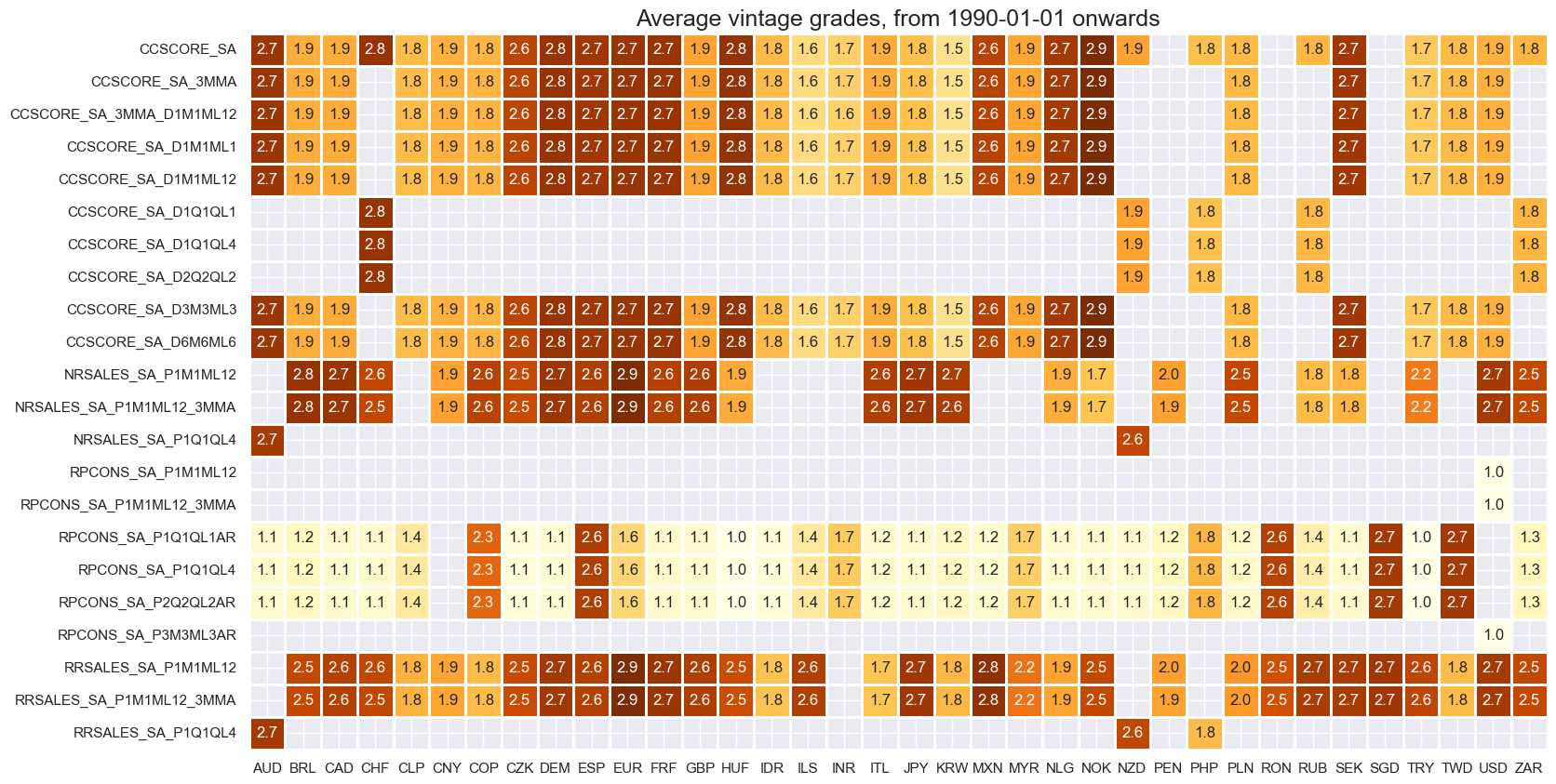
Average grades are currently quite mixed across countries and times. This reflects the availability of survey’s vintages and the use of multiple surveys used in some countries (USD for example).

xcatx = main
cidx = cids

plot = msp.heatmap_grades(
    df,
    xcats=xcatx,
    cids=cidx,
    start=start_date,
    size=(18, 10),
    title=f"Average vintage grades, from {start_date} onwards",
)

For graphical representation, it is helpful to rename some quarterly dynamics into an equivalent monthly dynamics.

dfx = df.copy()

dict_repl = {
    "CCSCORE_SA_D1Q1QL1": "CCSCORE_SA_D3M3ML3",
    "CCSCORE_SA_D2Q2QL2": "CCSCORE_SA_D6M6ML6",
    "CCSCORE_SA_D1Q1QL4": "CCSCORE_SA_3MMA_D1M1ML12",
    "NRSALES_SA_P1Q1QL4": "RRSALES_SA_3MMA_P1M1ML12",
    "RRSALES_SA_P1Q1QL4": "RRSALES_SA_3MMA_P1M1ML12",
    "RPCONS_SA_P1Q1QL4":  "RPCONS_SA_P1M1ML12_3MMA",   
    "RPCONS_SA_P1Q1QL1AR":"RPCONS_SA_P3M3ML3AR",
    "RPCONS_SA_P2Q2QL2AR":"RPCONS_SA_P6M6ML6AR",

}

for key, value in dict_repl.items():
    dfx["xcat"] = dfx["xcat"].str.replace(key, value)

History

Private consumption growth

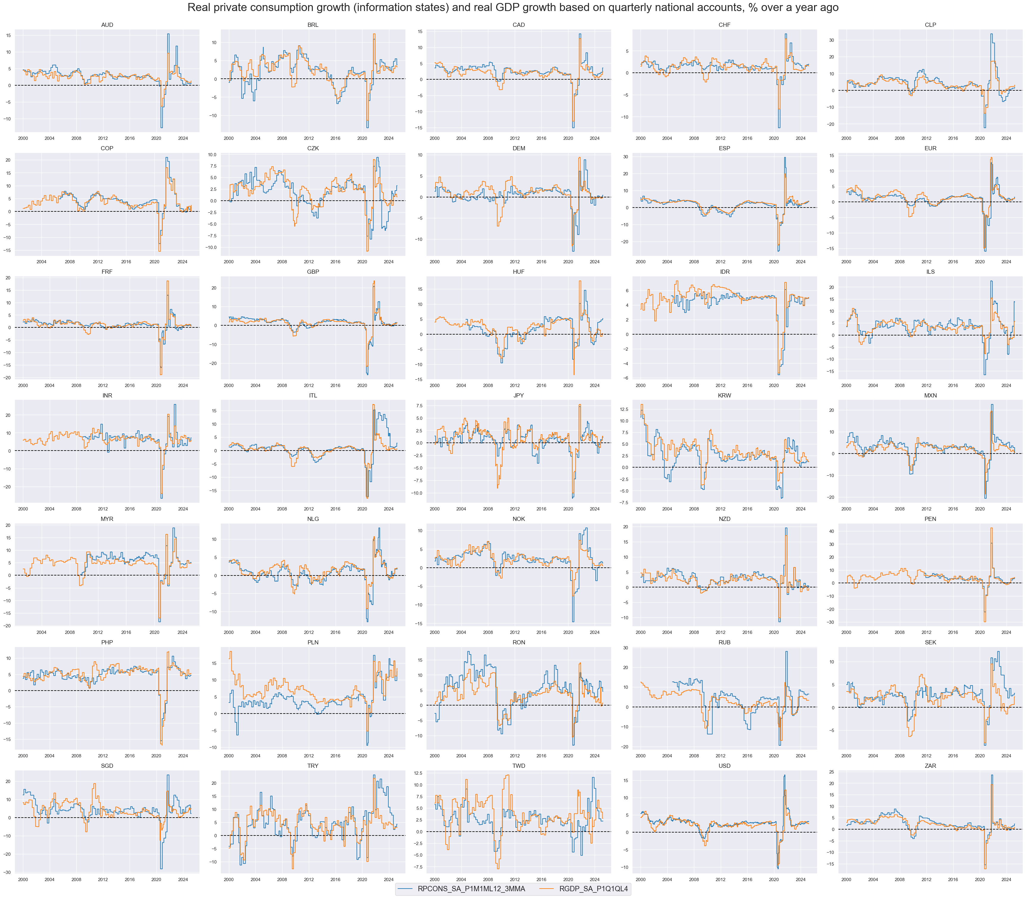
In developed countries real private consumption growth has historically been more stable than GDP growth. By contrast, in developed countries household spending post large fluctuations in crises and recoveries. Also the COVID pandemic has triggered outsized fluctuations of private consumption in almost all countries.

cidx = list(set(cids)- set(["CNY"]))  # exclude countries with monthly release
xcatx = [
    "RPCONS_SA_P1M1ML12_3MMA",
    "RGDP_SA_P1Q1QL4"
]

msp.view_timelines(
    dfx,
    xcats=xcatx,
    cids=cidx,
    start=start_date,
    title="Real private consumption growth (information states) and real GDP growth based on quarterly national accounts, % over a year ago",
    ncol=5,
    same_y=False,
    legend_fontsize=17,
    title_fontsize=27,
    size=(12, 7),
    all_xticks=True,
    legend_ncol=2,
 )

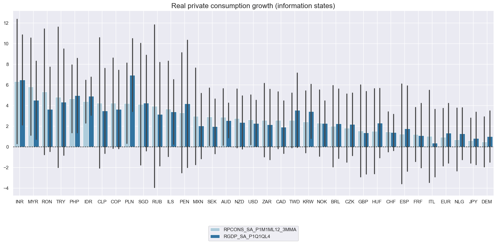
msp.view_ranges(
    dfx,
    xcats=xcatx,
    cids=cidx,
    sort_cids_by = "mean",
    start=start_date,
    title="Real private consumption growth (information states)",
    
 )

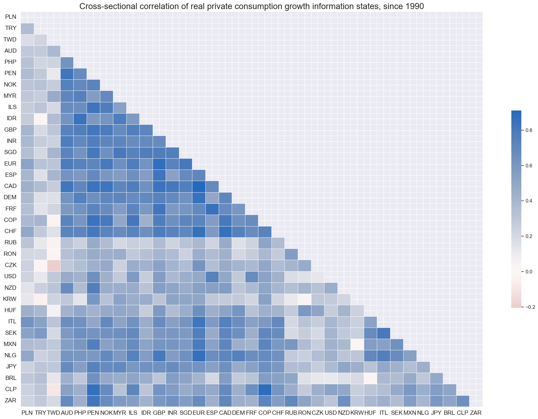
Reported private consumption growth has been positively correlated across almost all country pairs. Unlike for other economic indicators, the U.S. is the not the center of gravity for private consumption growth, probably reflecting the greater timeliness of the U.S. data.

msp.correl_matrix(
    dfx,
    xcats="RPCONS_SA_P1M1ML12_3MMA",
    cids=cids,
    size=(20, 14),
    start=start_date,
    freq="m",
    title="Cross-sectional correlation of real private consumption growth information states, since 1990",
    cluster=True,
)

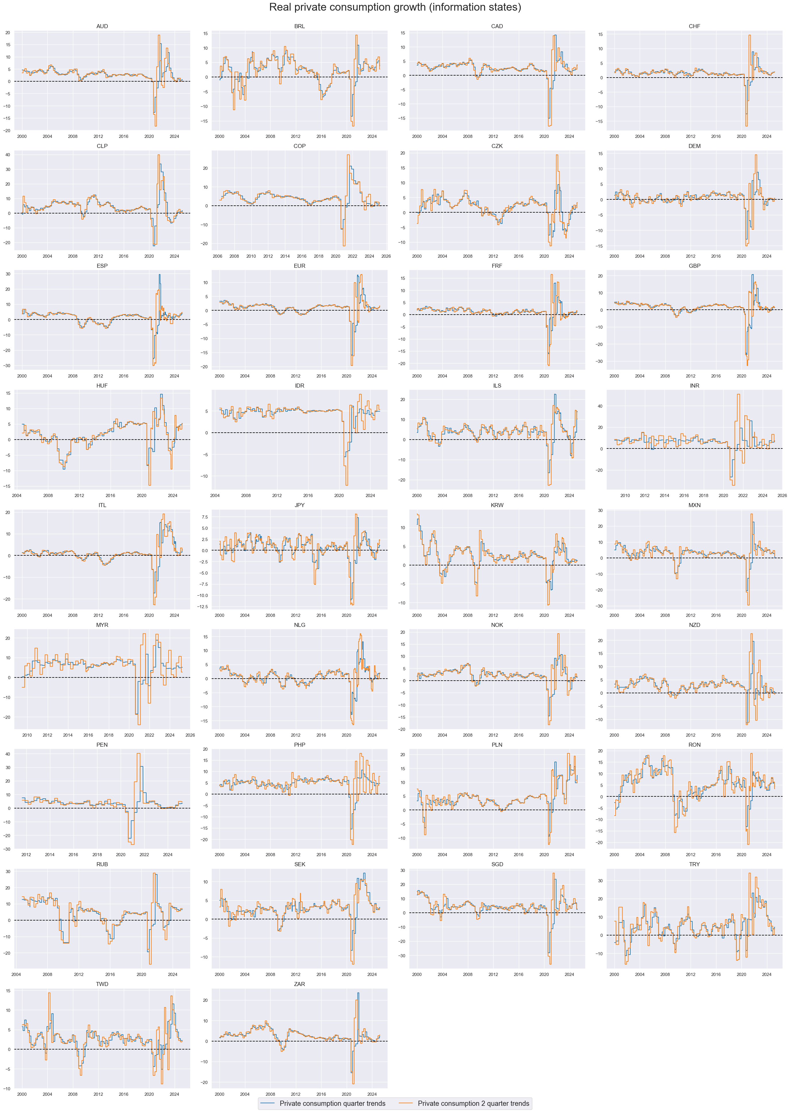
Quaterly and semi-annual consumption growth rates can be quite volatile, but still track broad business cycles.

cidx = list(set(cids) - set(["USD","CNY"]))  # exclude countries with quarterly surveys
xcatx = [
    "RPCONS_SA_P1M1ML12_3MMA",
    "RPCONS_SA_P6M6ML6AR",
]

msp.view_timelines(
    dfx,
    xcats=xcatx,
    cids=cidx,
    start=start_date,
    title="Real private consumption growth (information states)",
    xcat_labels=[
        "Private consumption quarter trends",
        "Private consumption 2 quarter trends",
    ],
    ncol=4,
    same_y=False,
    legend_fontsize=17,
    title_fontsize=27,
    size=(12, 7),
    all_xticks=True,
    legend_ncol=2,
)

Consumer confidence scores

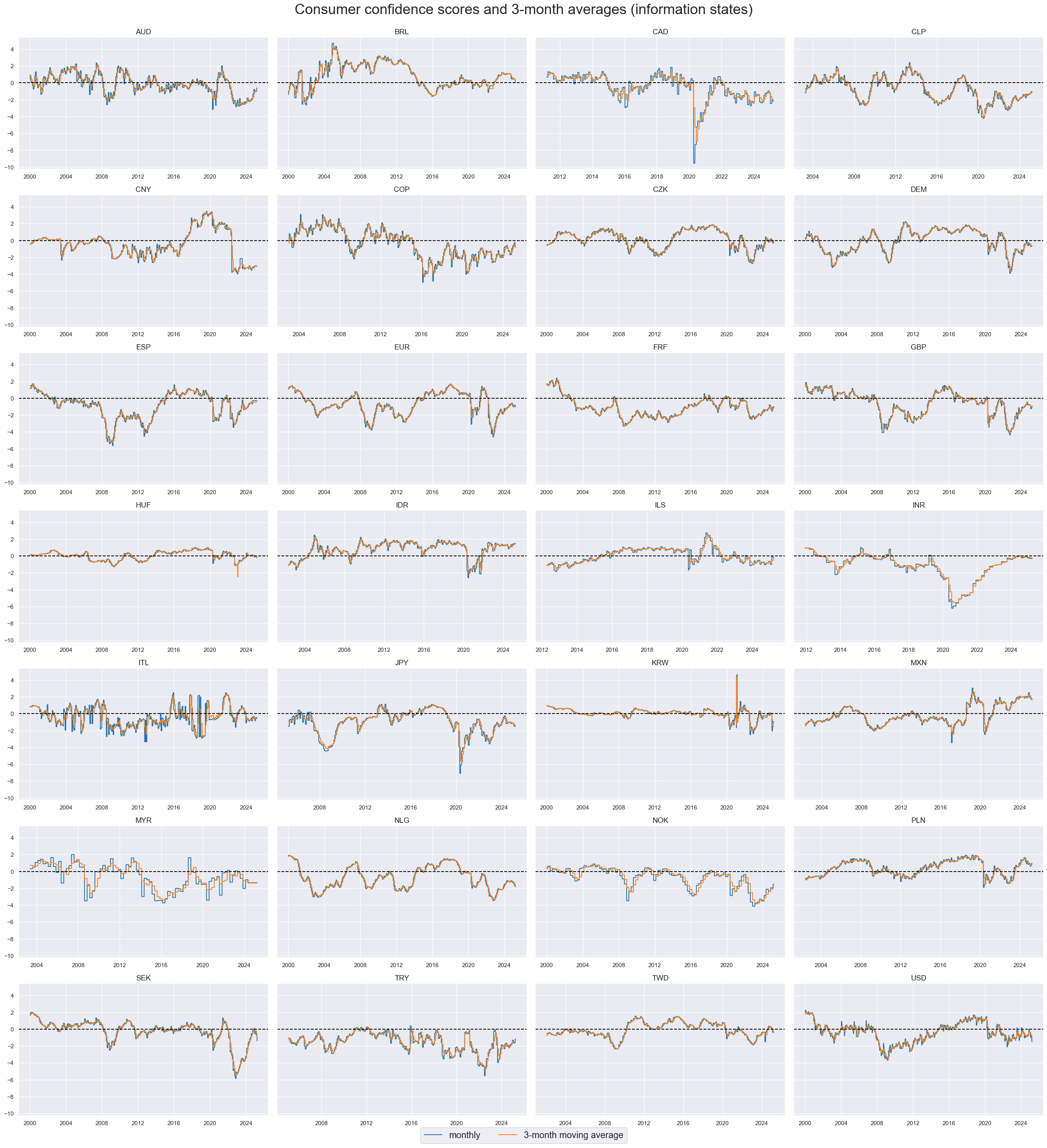
Consumer confidence level typically swing from positive to negative in multi-year cycles. Looking at 3-month moving average significantly adds to the stability of the indicators.

cidx = list(
    set(cids) - set(["CHF", "NZD", "PHP", "RUB", "ZAR","HKD","RON","SGD","PEN"])
)  # exclude countries with quarterly surveys
xcatx = ["CCSCORE_SA", "CCSCORE_SA_3MMA"]

msp.view_timelines(
    dfx,
    xcats=xcatx,
    cids=cidx,
    start=start_date,
    title="Consumer confidence scores and 3-month averages (information states)",
    xcat_labels=[
        "monthly",
        "3-month moving average",
    ],
    ncol=4,
    same_y=True,
    legend_fontsize=17,
    title_fontsize=27,
    size=(12, 7),
    all_xticks=True,
)

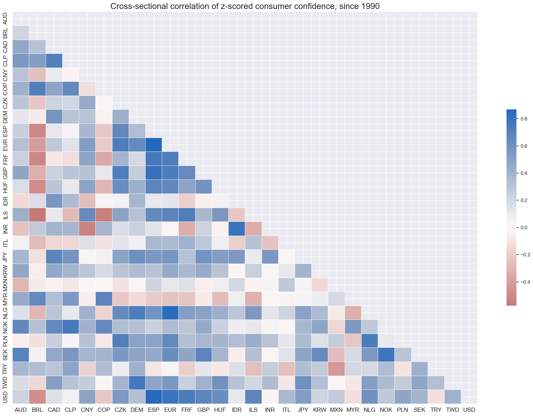
Correlation across (information states of) consumer confidence has not been uniformly positive around the world, with many emerging countries posting idiosyncratic dynamics, even vis-a-vis the dominant economies of the U.S. and the Euro area.

cidx = list(
    set(cids) - set(["CHF", "NZD", "PHP", "RUB", "ZAR", "HKD", "RON", "SGD", "PEN"])
)

msp.correl_matrix(

    dfx,

    xcats="CCSCORE_SA",
    cids=cidx,

    size=(20, 14),

    start=start_date,

    title="Cross-sectional correlation of z-scored consumer confidence, since 1990",
    freq="m",
)

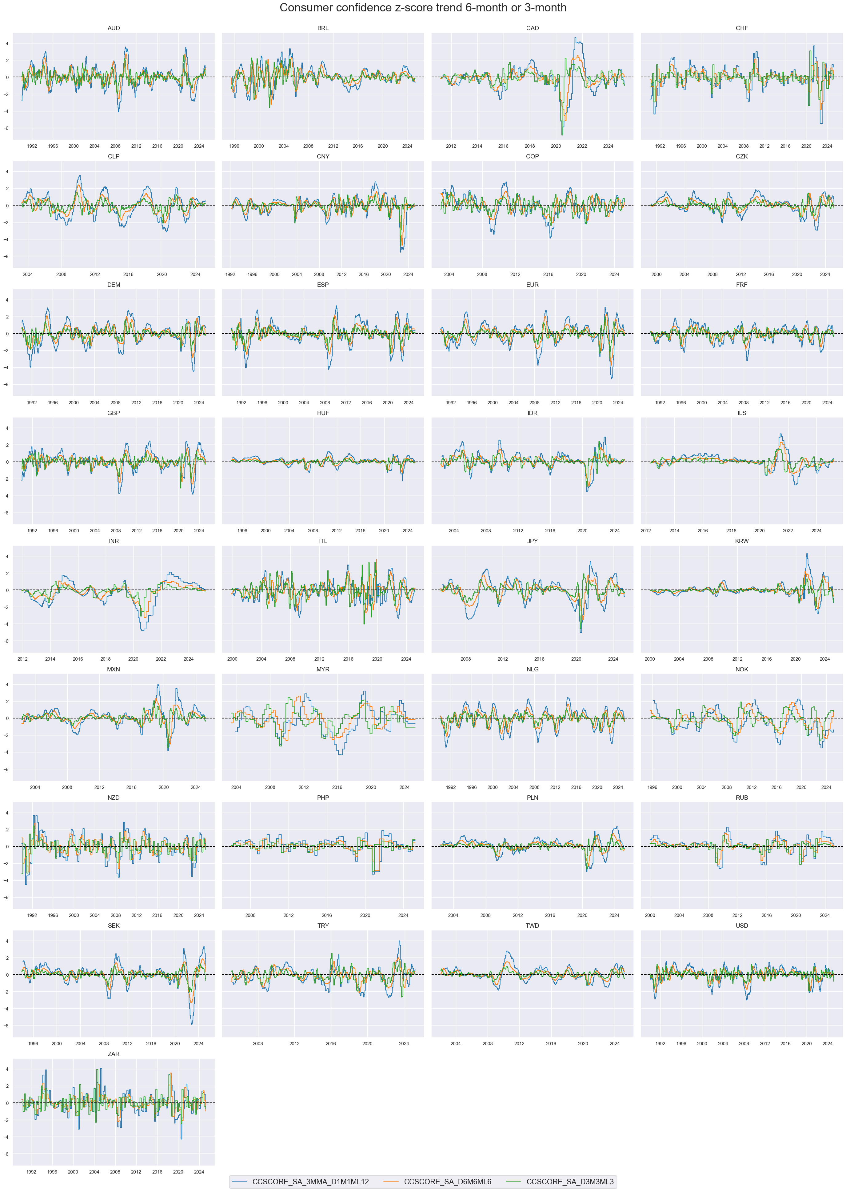
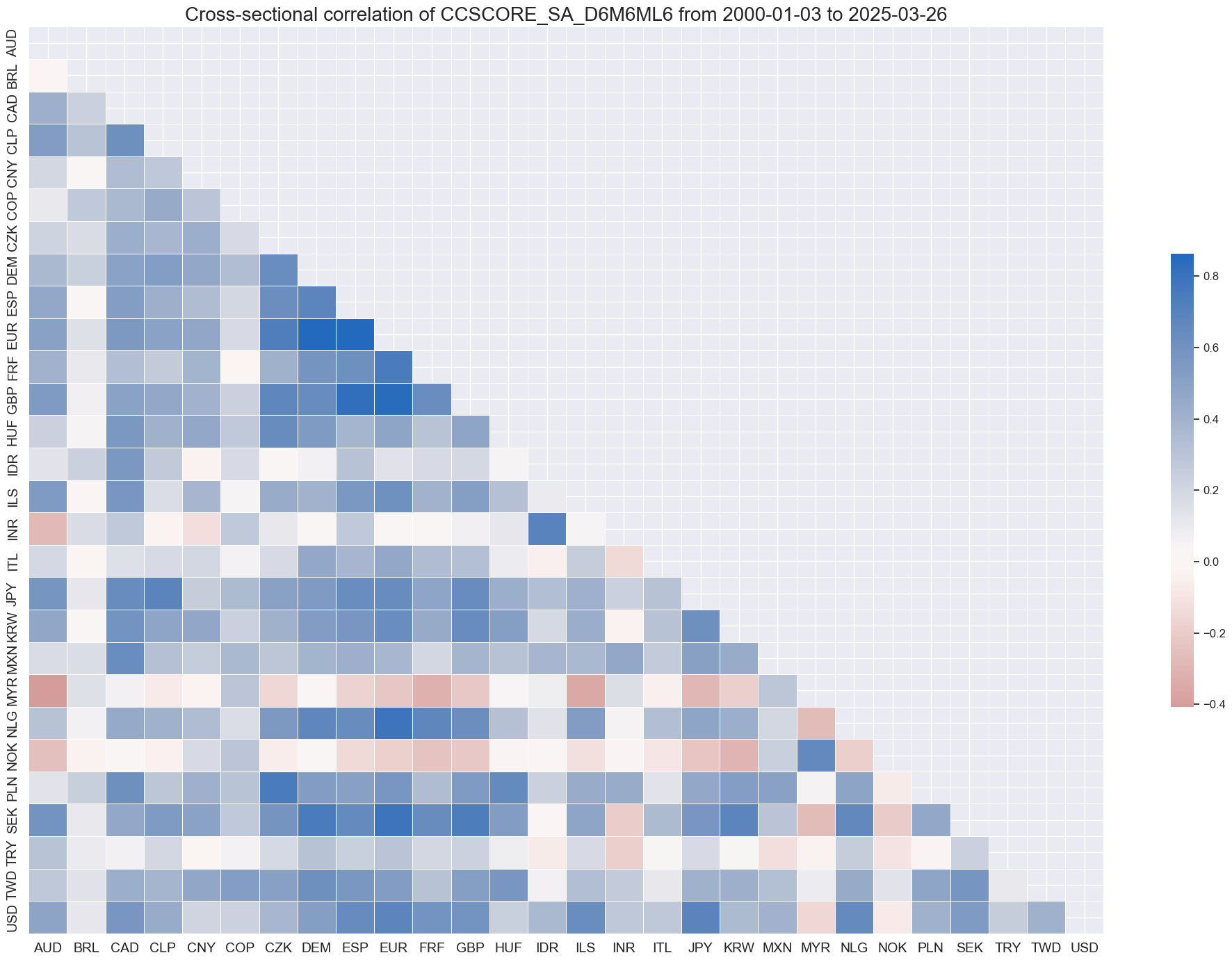
Consumer confidence score dynamics

Annual changes and changes of 6-month periods over the previous 6 months still seem to be consistent with business cycle fluctuations. Changes of the last three months over the previous three months can be quite volatile.

xcatx = ["CCSCORE_SA_3MMA_D1M1ML12", "CCSCORE_SA_D6M6ML6", "CCSCORE_SA_D3M3ML3"]
cidx = cids

msp.view_timelines(
    dfx,
    xcats=xcatx,
    cids=cidx,
    start=start_date,
    title="Consumer confidence z-score trend 6-month or 3-month",
    legend_fontsize=17,
    title_fontsize=27,
    ncol=4,
    same_y=True,
    size=(12, 7),
    all_xticks=True,
)

Interestingly, changes in consumer confidence are more correlated across countries than the levels themselves.

msp.correl_matrix(df, xcats="CCSCORE_SA_D6M6ML6", cids=cidx, size=(20, 14))

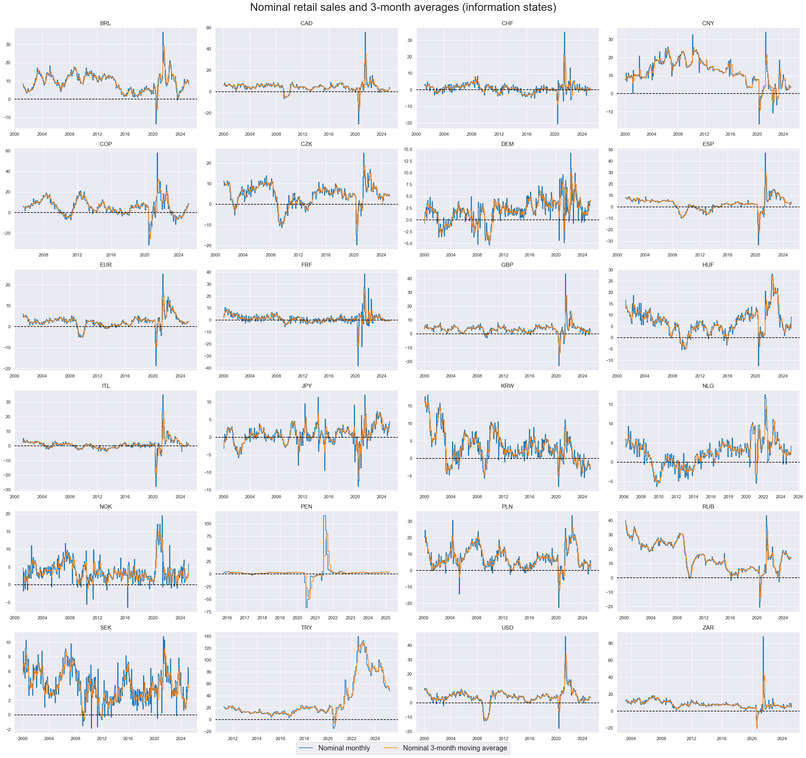
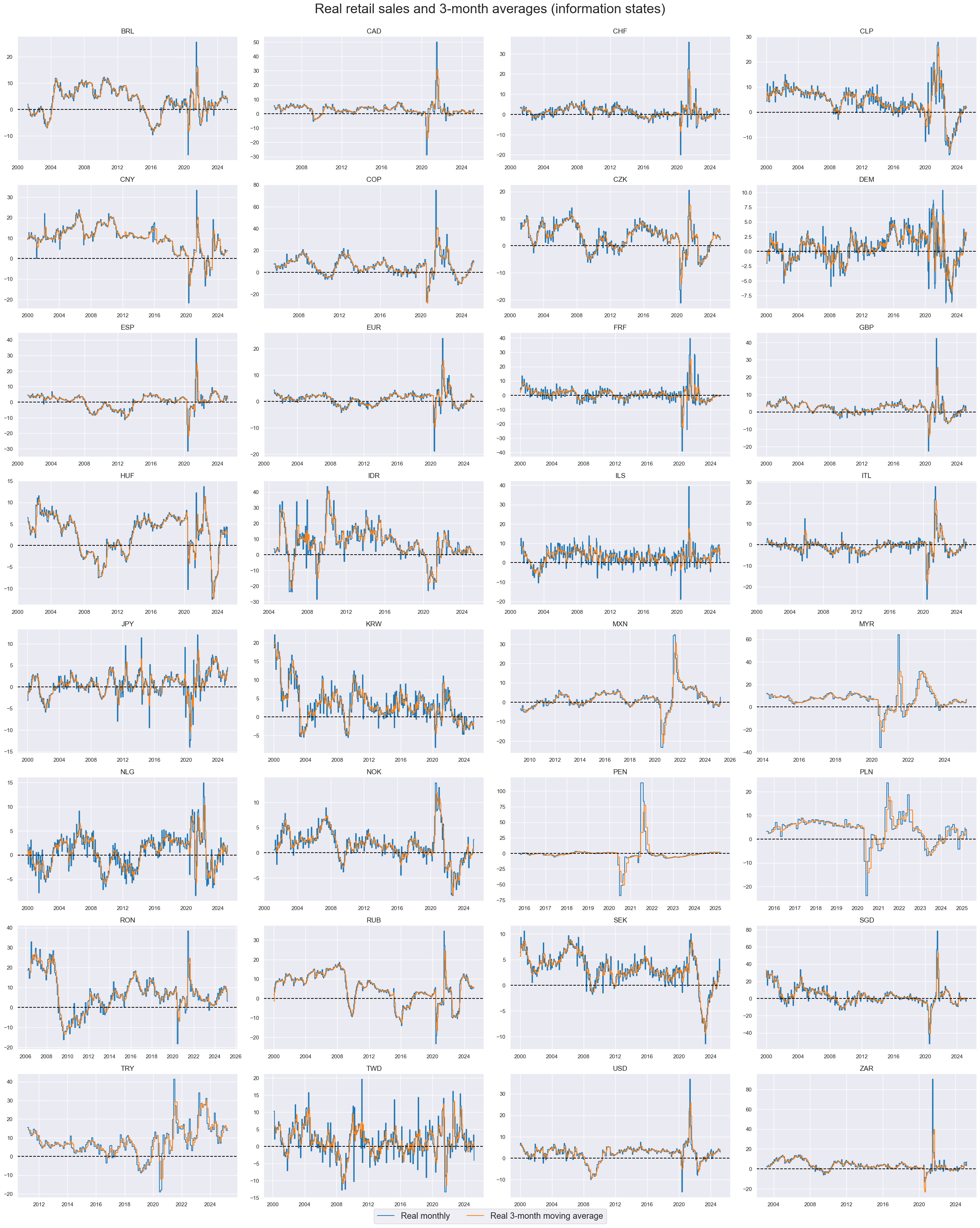
Retail sales growth

Averaging of monthly growth rates of nominal or real retail sales gorwth is very useful for detecting information states of more stable trends. In countries with escalating inflation, such as Turkey in the early 2020s, CPI growth dominates volume dynamics.

cidx = list(set(cids) - set(["NZD", "AUD"]))  # exclude countries with quarterly surveys
xcatx = [
    "NRSALES_SA_P1M1ML12",
    "NRSALES_SA_P1M1ML12_3MMA",
]

msp.view_timelines(
    dfx,
    xcats=xcatx,
    cids=cidx,
    start=start_date,
    title="Nominal retail sales and 3-month averages (information states)",
    xcat_labels=[
        "Nominal monthly",
        "Nominal 3-month moving average",
    ],
    ncol=4,
    same_y=False,
    legend_fontsize=17,
    title_fontsize=27,
    size=(12, 7),
    all_xticks=True,
    legend_ncol=2,
)

cidx = list(set(cids) - set(["NZD", "AUD"]))  # exclude countries with quarterly surveys
xcatx = ["RRSALES_SA_P1M1ML12", "RRSALES_SA_P1M1ML12_3MMA"]

msp.view_timelines(
    dfx,
    xcats=xcatx,
    cids=cidx,
    start=start_date,
    title="Real retail sales and 3-month averages (information states)",
    xcat_labels=[
        "Real monthly",
        "Real 3-month moving average"],
    ncol=4,
    same_y=False,
    legend_fontsize=17,
    title_fontsize=27,
    size=(12, 7),
    all_xticks=True,
    legend_ncol=2,
)

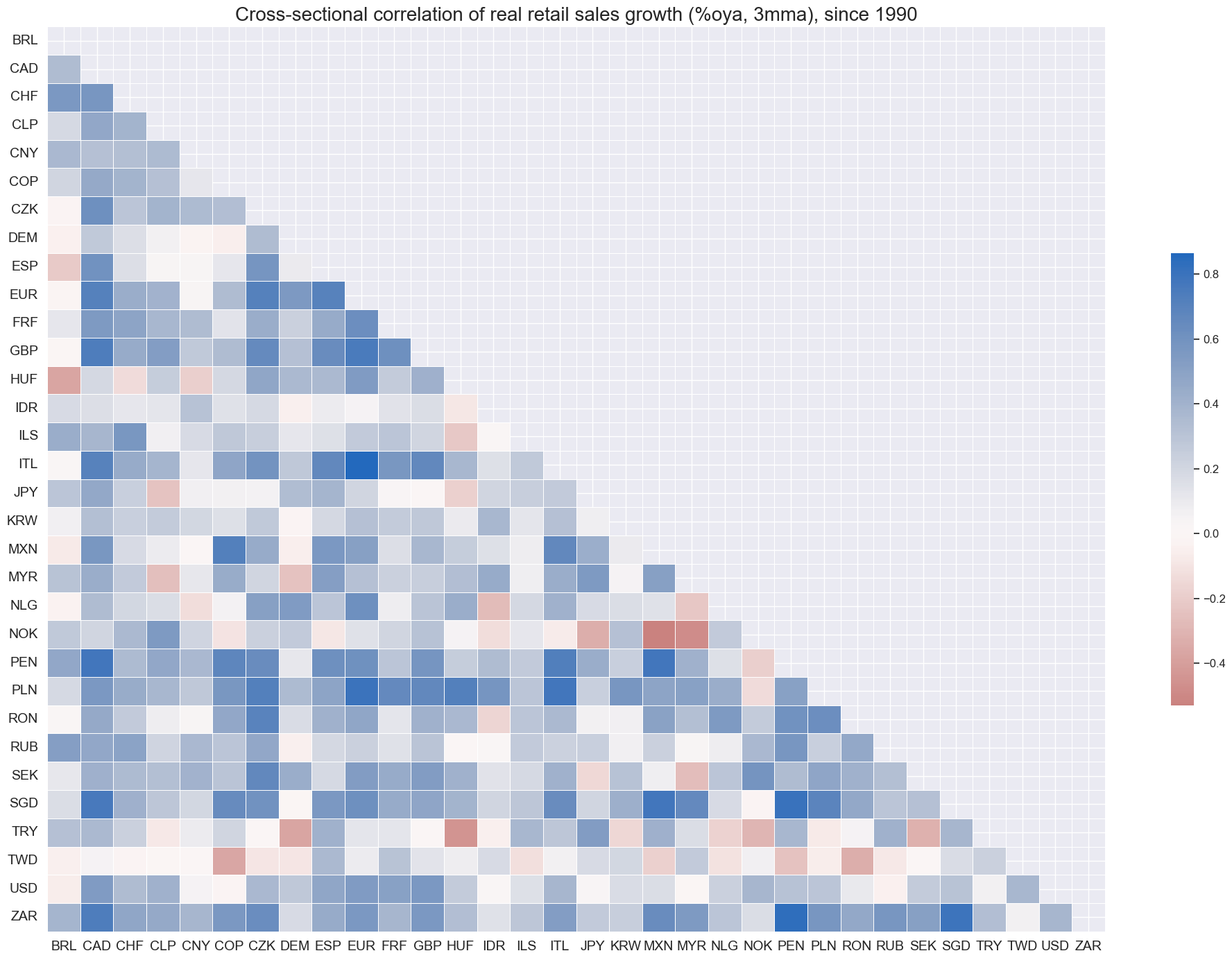
Retail sales growth is mostly positively correlated across most countries.

msp.correl_matrix(
    dfx,
    xcats="RRSALES_SA_P1M1ML12_3MMA",
    cids=cidx,
    size=(20, 14),
    start=start_date,
    title="Cross-sectional correlation of real retail sales growth (%oya, 3mma), since 1990",
)

Importance

Research links

“The interaction between the macroeconomy and asset markets is central to a variety of modern theories of the business cycle. Much recent work emphasizes the joint nature of the consumption decision and the portfolio allocation decision.” Mankiw and Shapiro

on consumption and stock returns

“… consumption-based predictive variable, called cyclical consumption … captures a significant fraction of variation in expected stock returns” Atanasov, Vinther Moeller and Priestley

“… the marginal utility of consumption, when suitably modeled, can explain the trade-off between risk and returnreflected in the size premium, the value premium, and the time-varying equity” M Yogo

“… Using U.S. quarterly stock market data, we find that these fluctuations in the consumption-wealth ratio are strong predictors of both real stock returns and excess returns over a Treasury bill rate” Lettau and Ludvigson

“When consumption falls, expected returns, return volatility, and the price of risk rise, and price/dividend ratios decline. “ Campbell and Cochrane

on consumption and bond returns

“We find that, for our sample, the risk related to long run prospects in future consumption plays a crucial role in pricing nominal US government bonds. Risk premium related to that source or risk if found to be positive and statistically significant.” Abhyankar, Klinkowska and Lee

“… a positive shock to consumption volatility move the expected excess bond returns and the yield-spread in the same direction” Bansaland Shaliastovich

on consumption and currency returns

“We find a strong link between currency excess returns and the relative strength of the business cycle. Buying currencies of strong economies and selling currencies of weak economies generates high returns both in the cross-section and time series of countries.” Colacito, Riddiough and Sarno

on consumption and commodity returns

“Our empirical analysis shows that changes in consumption and inventory are strongly related, but that under certain conditions, consumption changes have direct effects on futures prices and volatility that are not mediated through changes in inventory.” Sklibosios Nikitopoulos, Squires, Thorp and Yeung

“Empirical studies have documented the time-varying correlation between returns on the market portfolio of stocks and those on long-term (5-10 years) nominal Treasury bonds. This correlation was positive before 2000 but turned negative afterwards (see chart below). At the same time, the correlation between consumption growth and inflation also changed sign around 2000 from negative to positive.” Li, Tao, Ji and Hao, 2021

Empirical clues new

Private consumption as a predictor of IRS returns

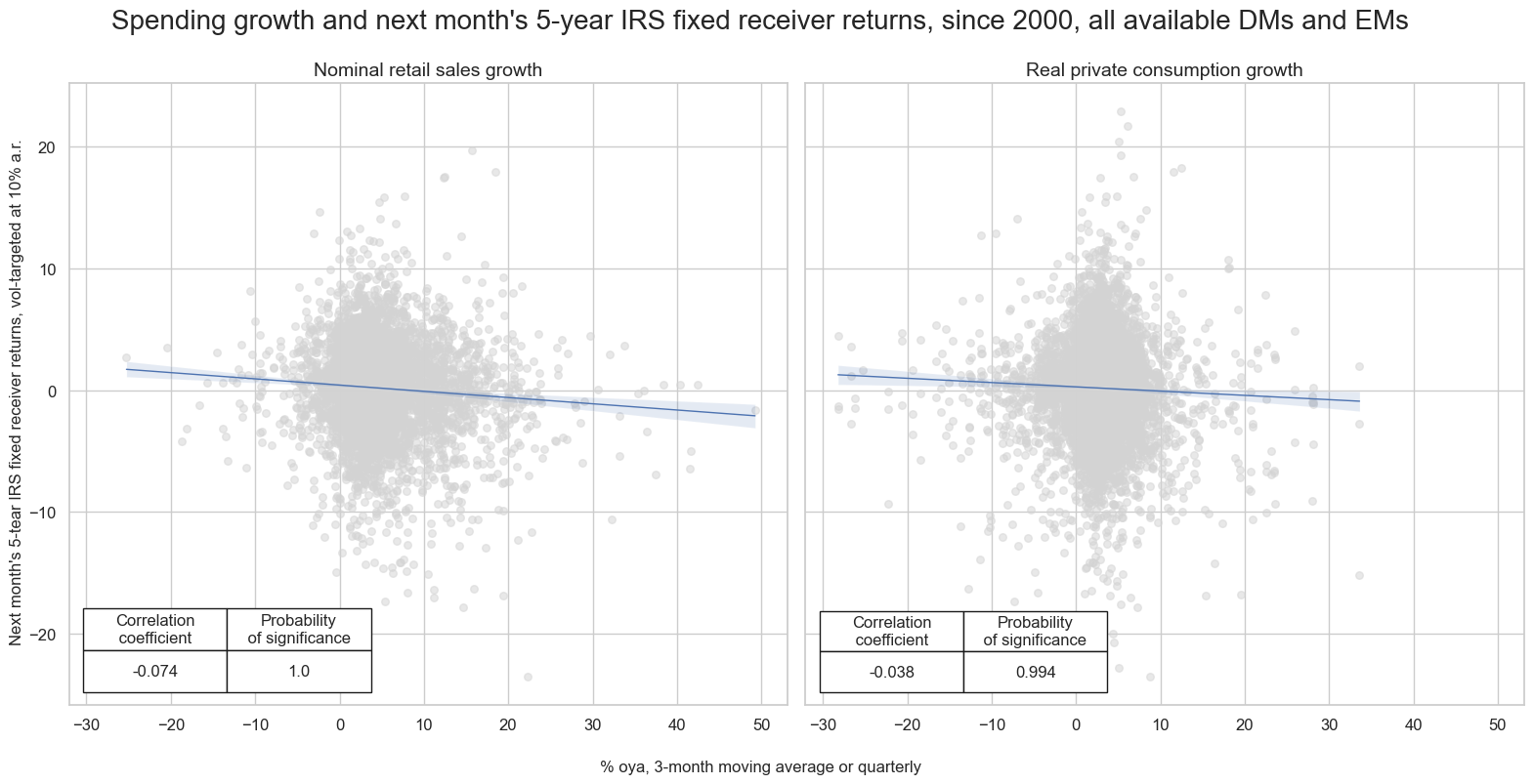
Point-in-time information states of both nominal retail sales growth and real private consumption growth have been highly significant negative predictors of subsequent monthly duration returns across developed and emerging markets, both across countries and across time This is consistent with standard economic theory that posits that central bank will seek to stabilize final sales growth in the economy in order to pursue inflation and economic growth objectives. The predictive power of nominal retail sales growth is particularly strong, reflecting that this indicator contains information on both the volume and price of goods sold.

targ = "DU05YXR_VT10"
cidx = cids_dmca + cids_em

cr_rs = msp.CategoryRelations(
    dfx,
    xcats=["NRSALES_SA_P1M1ML12_3MMA", targ],
    cids=cidx,
    freq="m",
    lag=1,
    xcat_aggs=["last", "sum"],
    start="2000-01-01",
    xcat_trims=(50, 25)  # for plot focus
)

cr_co = msp.CategoryRelations(
    dfx,
    xcats=["RPCONS_SA_P1M1ML12_3MMA", targ],
    cids=cidx,
    freq="m",
    lag=1,
    xcat_aggs=["last", "sum"],
    start="2000-01-01",
    xcat_trims=(50, 25)  # for plot focus
)


msv.multiple_reg_scatter(
        [cr_rs, cr_co],
        title="Spending growth and next month's 5-year IRS fixed receiver returns, since 2000, all available DMs and EMs" ,
        xlab="% oya, 3-month moving average or quarterly",
        ylab="Next month's 5-tear IRS fixed receiver returns, vol-targeted at 10% a.r.",
        ncol=2,
        nrow=1,
        figsize=(16, 8),
        prob_est="map",
        coef_box="lower left", 
        subplot_titles=["Nominal retail sales growth", "Real private consumption growth"],
     )

NRSALES_SA_P1M1ML12_3MMA misses: ['AUD', 'CLP', 'HKD', 'IDR', 'ILS', 'INR', 'MXN', 'MYR', 'NZD', 'PHP', 'RON', 'SGD', 'TWD'].
DU05YXR_VT10 misses: ['PEN', 'PHP', 'RON'].
RPCONS_SA_P1M1ML12_3MMA misses: ['CNY', 'HKD'].
DU05YXR_VT10 misses: ['PEN', 'PHP', 'RON'].

Consumer confidence as a predictor of equity returns

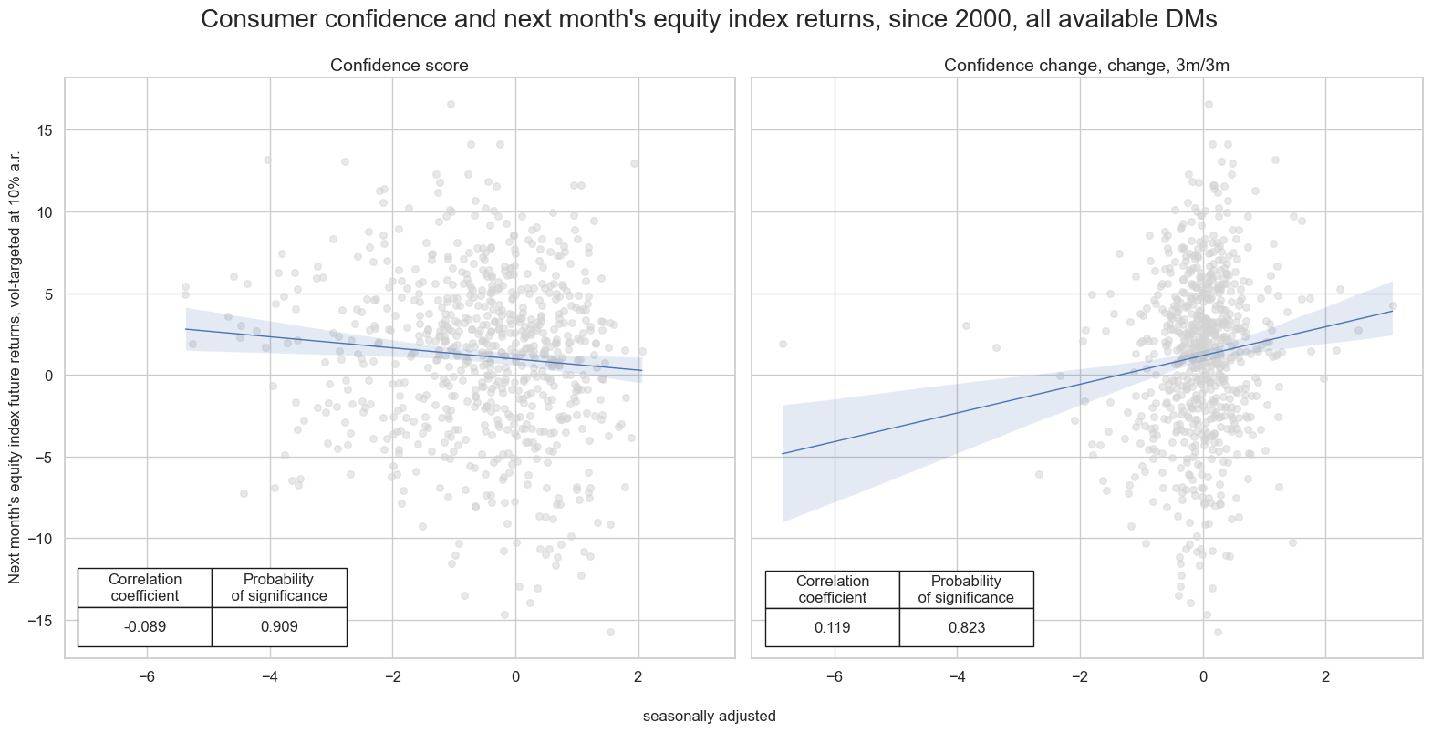
In the developed markets there has been a “double relation” between the information state of consumer confidence and subsequent returns. The level of confidence has negatively predicted returns, while short-term changes have been a positive signal. This may reflect that confidence level mostly reflect the state of the business cycle (with high levels calling for policy tightening), while changes indicate actual sentiment shifts (with increases supporting positive sentiment in financial markets)

targ = "EQXR_VT10"
cidx = cids_dmeq

cr_cs = msp.CategoryRelations(
    dfx,
    xcats=["CCSCORE_SA", targ],
    cids=cidx,
    freq="q",
    lag=1,
    xcat_aggs=["last", "sum"],
    start="2000-01-01",
)

cr_cd = msp.CategoryRelations(
    dfx,
    xcats=["CCSCORE_SA_D3M3ML3", targ],
    cids=cidx,
    freq="q",
    lag=1,
    xcat_aggs=["last", "sum"],
    start="2000-01-01",
)


msv.multiple_reg_scatter(
        [cr_cs, cr_cd],
        title="Consumer confidence and next month's equity index returns, since 2000, all available DMs" ,
        xlab="seasonally adjusted",
        ylab="Next month's equity index future returns, vol-targeted at 10% a.r.",
        ncol=2,
        nrow=1,
        figsize=(16, 8),
        prob_est="map",
        coef_box="lower left", 
        subplot_titles=["Confidence score", "Confidence change, change, 3m/3m"],
     )

CCSCORE_SA misses: ['HKD', 'SGD'].
EQXR_VT10 misses: ['ILS', 'NOK', 'NZD'].
CCSCORE_SA_D3M3ML3 misses: ['HKD', 'SGD'].
EQXR_VT10 misses: ['ILS', 'NOK', 'NZD'].

Private consumption as a predictor of equity sector returns

# Adjusting by untradability flag: where flag=1 values are set to NaNs

# support column for the category match
dfx['sector'] = dfx['xcat'].str[0:6]

# finding untradable category
untradable_df = dfx.loc[dfx['xcat'].str.endswith('UNTRADABLE_NSA'), :]
# finding return categories
ret_df = dfx.loc[dfx['xcat'].isin(eqret), :]

# excluding it from the target dataset
dfx = dfx.loc[
    (~dfx['xcat'].str.endswith('UNTRADABLE_NSA')) & (~dfx['xcat'].isin(eqret))
]
# merging the two
ret_df = ret_df.merge(
    untradable_df.loc[:, ['real_date', 'cid', 'sector', 'value']].rename(columns={'value': 'untrad'}), 
    on=['real_date', 'cid', 'sector'], 
    how='left'
)

# finding where indices have no constituents
mask = (ret_df['untrad'] == 1)
ret_df.loc[mask, 'value'] = np.NaN

# cleaning
ret_df = ret_df.drop(columns=['untrad', 'sector'])

# re-adding the returns back into dfd
dfx = msm.update_df(dfx, ret_df)
#xcats = list(set(xcats) - set(untradable))

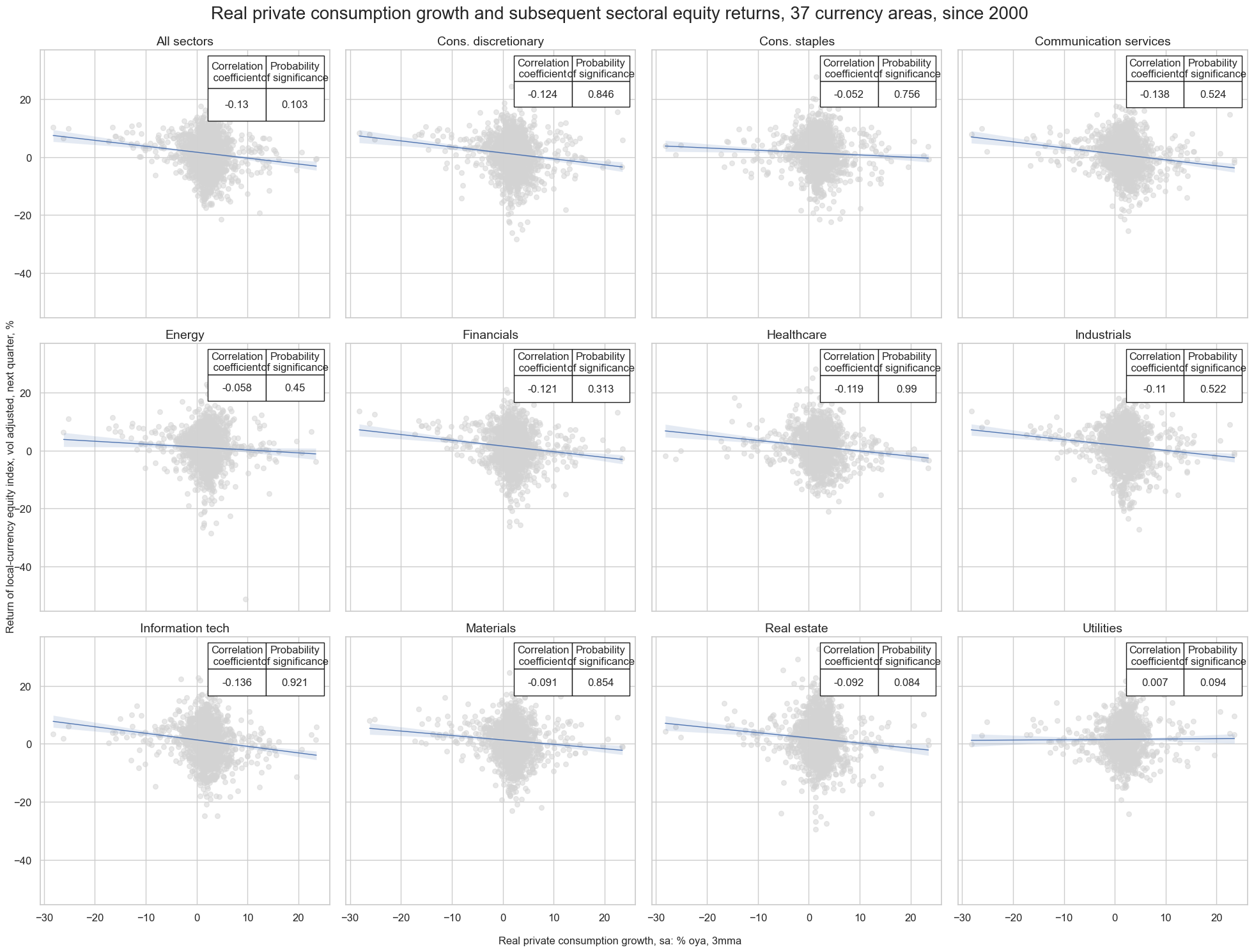
The predictive relationship between private consumption growth and equity returns has been negative across most sectos, except for (highly regulated) utilities sector.

#cidx = list(set(cids_dmeq) - set(["HKD"]))

start_date = "2000-01-01"

sector_dict = {}

for sector in sectors:
    # Define the category pair
    xcatx = ["RPCONS_SA_P1M1ML12_3MMA", f"EQC{sector}XR_VT10"]
    
    # Compute category relations for the sector
    sector_cr = msp.CategoryRelations(
        dfx,
        xcats=xcatx,
        cids=list(set(sector_cids) - set(["HKD"])),  # HKD not available
        freq="Q",
        lag=1,
        xcat_aggs=["last", "sum"],
        start=start_date
    )
    
    # Store the result in the dictionary
    sector_dict[sector] = sector_cr

msv.multiple_reg_scatter(
    cat_rels=list(sector_dict.values()),
    ncol=4,
    nrow=3,
    figsize=(20, 15),
    title=f"Real private consumption growth and subsequent sectoral equity returns, {len(cids)} currency areas, since 2000",
    title_fontsize=20,
    xlab="Real private consumption growth, sa: % oya, 3mma",
    ylab="Return of local-currency equity index, vol adjusted, next quarter, %",
    coef_box="upper right",
    prob_est="map",
    single_chart=True,
    subplot_titles=[sector_labels[sector] for sector in sectors]
)

EQCENRXR_VT10 misses: ['CHF'].

Private consumption and FX returns

dfb = df[df["xcat"].isin(["FXTARGETED_NSA", "FXUNTRADABLE_NSA"])].loc[
    :, ["cid", "xcat", "real_date", "value"]
]
dfba = (
    dfb.groupby(["cid", "real_date"])
    .aggregate(value=pd.NamedAgg(column="value", aggfunc="max"))
    .reset_index()
)
dfba["xcat"] = "FXBLACK"
fxblack = msp.make_blacklist(dfba, "FXBLACK")
fxblack

{'BRL': (Timestamp('2012-12-03 00:00:00'), Timestamp('2013-09-30 00:00:00')),
 'CHF': (Timestamp('2011-10-03 00:00:00'), Timestamp('2015-01-30 00:00:00')),
 'CNY': (Timestamp('1999-01-01 00:00:00'), Timestamp('2024-12-16 00:00:00')),
 'CZK': (Timestamp('2014-01-01 00:00:00'), Timestamp('2017-07-31 00:00:00')),
 'HKD': (Timestamp('1999-01-01 00:00:00'), Timestamp('2024-12-16 00:00:00')),
 'ILS': (Timestamp('1999-01-01 00:00:00'), Timestamp('2005-12-30 00:00:00')),
 'INR': (Timestamp('1999-01-01 00:00:00'), Timestamp('2004-12-31 00:00:00')),
 'MYR_1': (Timestamp('1999-01-01 00:00:00'), Timestamp('2007-11-30 00:00:00')),
 'MYR_2': (Timestamp('2018-07-02 00:00:00'), Timestamp('2024-12-16 00:00:00')),
 'PEN': (Timestamp('2021-07-01 00:00:00'), Timestamp('2021-07-30 00:00:00')),
 'RON': (Timestamp('1999-01-01 00:00:00'), Timestamp('2005-11-30 00:00:00')),
 'RUB_1': (Timestamp('1999-01-01 00:00:00'), Timestamp('2005-11-30 00:00:00')),
 'RUB_2': (Timestamp('2022-02-01 00:00:00'), Timestamp('2024-12-16 00:00:00')),
 'SGD': (Timestamp('1999-01-01 00:00:00'), Timestamp('2024-12-16 00:00:00')),
 'TRY_1': (Timestamp('1999-01-01 00:00:00'), Timestamp('2003-09-30 00:00:00')),
 'TRY_2': (Timestamp('2020-01-01 00:00:00'), Timestamp('2024-07-31 00:00:00'))}

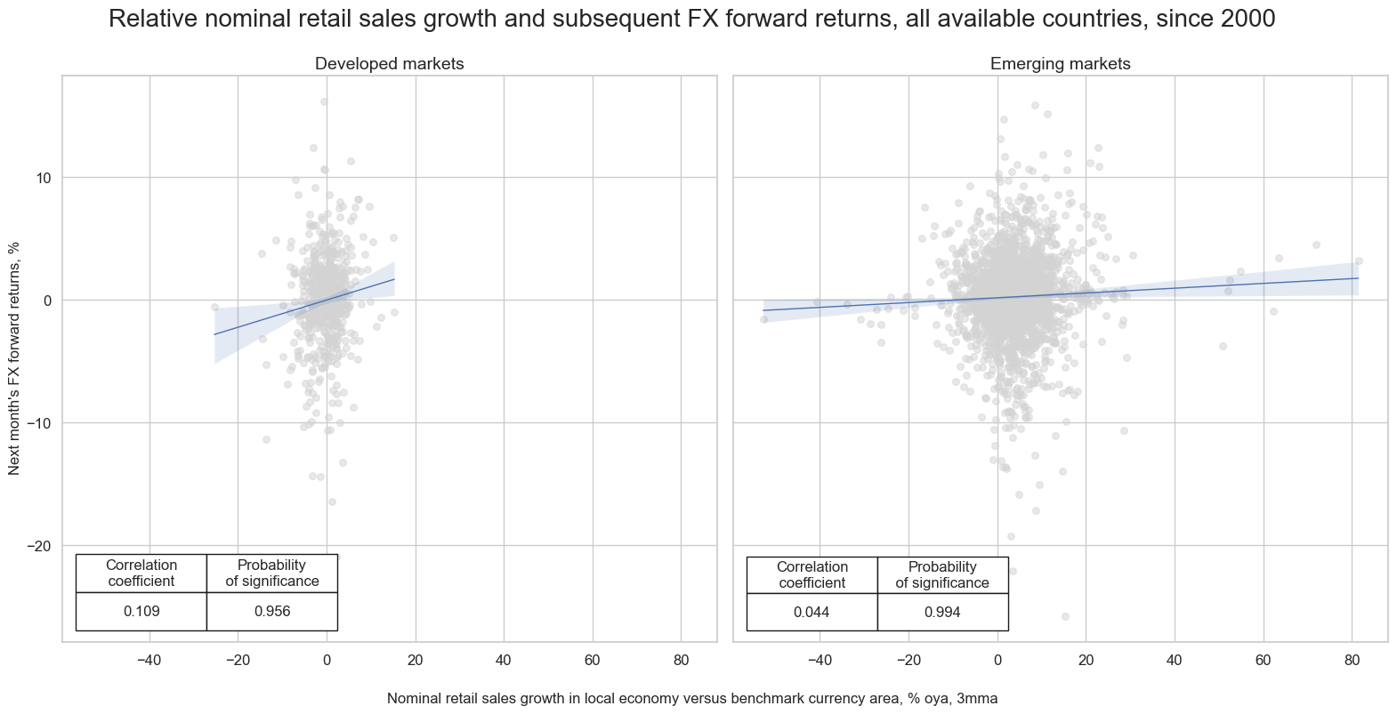
Differentials of (nominal) retail sales growth in local economies and benchmark currency areas (i.e., U.S. and Euro area) have been a significant predictor of subsequent FX returns. This holds true for both developed and emerging economies and is consistent with the idea that most central banks will seek to stabilize nominal final sales growth in the economy in order to pursue inflation and economic growth objectives.

xcatx = ["NRSALES_SA_P1M1ML12_3MMA"]
         
dfa = pd.DataFrame(columns=list(dfx.columns))


for xc in xcatx:
    calc_eur = [f"{xc}vBM = {xc} - iEUR_{xc}"]
    calc_usd = [f"{xc}vBM = {xc} - iUSD_{xc}"]
    calc_eud = [f"{xc}vBM = {xc} - 0.5 * ( iEUR_{xc} + iUSD_{xc} )"]

    dfa_eur = msp.panel_calculator(dfx, calcs=calc_eur, cids=cids_eur)
    dfa_usd = msp.panel_calculator(dfx, calcs=calc_usd, cids=cids_usd)
    dfa_eud = msp.panel_calculator(dfx, calcs=calc_eud, cids=cids_eud)

    dfa = msm.update_df(dfa, pd.concat([dfa_eur, dfa_usd, dfa_eud]))

dfx = msm.update_df(dfx, dfa)

cidx = cids_dmca

cr_dm = msp.CategoryRelations(
    dfx,
    xcats=["NRSALES_SA_P1M1ML12_3MMAvBM", "FXXR_NSA"],
    cids=cids_dmfx,
    freq="q",
    lag=1,
    xcat_aggs=["last", "sum"],
    start="2000-01-01",
    blacklist=fxblack,
)

cr_em = msp.CategoryRelations(
    dfx,
    xcats=["NRSALES_SA_P1M1ML12_3MMAvBM", "FXXR_NSA"],
    cids=cids_emfx,
    freq="m",
    lag=1,
    xcat_aggs=["last", "sum"],
    start="2000-01-01",
    blacklist=fxblack,
)

msv.multiple_reg_scatter(
        [cr_dm, cr_em],
        title="Relative nominal retail sales growth and subsequent FX forward returns, all available countries, since 2000" ,
        xlab="Nominal retail sales growth in local economy versus benchmark currency area, % oya, 3mma",
        ylab="Next month's FX forward returns, %",
        ncol=2,
        nrow=1,
        figsize=(16, 8),
        prob_est="map",
        coef_box="lower left", 
        subplot_titles=["Developed markets", "Emerging markets"],
     )

NRSALES_SA_P1M1ML12_3MMAvBM misses: ['AUD', 'NZD'].
NRSALES_SA_P1M1ML12_3MMAvBM misses: ['CLP', 'HKD', 'IDR', 'ILS', 'INR', 'MXN', 'MYR', 'PHP', 'RON', 'TWD'].
FXXR_NSA misses: ['HKD'].

Appendices

Appendix 1: Currency symbols

The word ‘cross-section’ refers to currencies, currency areas or economic areas. In alphabetical order, these are AUD (Australian dollar), BRL (Brazilian real), CAD (Canadian dollar), CHF (Swiss franc), CLP (Chilean peso), CNY (Chinese yuan renminbi), COP (Colombian peso), CZK (Czech Republic koruna), DEM (German mark), ESP (Spanish peseta), EUR (Euro), FRF (French franc), GBP (British pound), HKD (Hong Kong dollar), HUF (Hungarian forint), IDR (Indonesian rupiah), ITL (Italian lira), JPY (Japanese yen), KRW (Korean won), MXN (Mexican peso), MYR (Malaysian ringgit), NLG (Dutch guilder), NOK (Norwegian krone), NZD (New Zealand dollar), PEN (Peruvian sol), PHP (Phillipine peso), PLN (Polish zloty), RON (Romanian leu), RUB (Russian ruble), SEK (Swedish krona), SGD (Singaporean dollar), THB (Thai baht), TRY (Turkish lira), TWD (Taiwanese dollar), USD (U.S. dollar), ZAR (South African rand).

Appendix 2: Methodology of scoring

Survey confidence values are transformed into z-scores based on past expanding data samples in order to replicate the market’s information state on survey readings relative to what is considered as “normal”.

The underlying economic data used to develop the above indicators comes in the form of diffusion index or derivatives thereof. They are either seasonally adjusted at the source or by JPMaQS. This statistic is typically used to summarise surveys results with focus on the direction of conditions (extensive margin) rather than the quantity (intensive margin).

In order to standardise different survey indicators, we apply a custom z-scoring methodology to each survey’s vintage based on the principle of a sliding scale for the weights of empirical versus theoretical neutral level:

• We first determine a theoretical nominal neutral level, defined by the original formula used by the publishing institution. This is typically one of 0, 50, or 100.

• We compute the measure of central tendency: for the first 5 years this is a weighted average of neutral level and realised median. As time progresses, the weight of the historical median increases and the weight of the notional neutral level decreases until it reaches zero at the end of the 5-year period.,

• We compute the mean absolute deviation to normalize deviations of confidence levels from their presumed neutral level. We require at least 12 observations to estimate it.

We finally calculate the z-score for the vintage values as

\[ Z_{i, t} = \frac{X_{i, t} - \bar{X_i|t}}{\sigma_i|t} \]

where \(X_{i, t}\) is the value of the indicator for country \(i\) at time \(t\) , \(\bar{X_i|t}\) is the measure of central tendency for country \(i\) at time \(t\) based on information up to that date, and \(\sigma_i|t\) is the mean absolute deviation for country \(i\) at time \(t\) based on information up to that date. Whenever a country / currency area has more than one representative survey, we average the z-scores by observation period (month or quarter).

We want to maximise the use of information set at each point in time, so we devised a back-casting algorithm to estimate a z-scored diffusion index in case another survey has already released some data for the latest observation period. Put simply, as soon as one survey for a month has been published we estimated the value for the other(s) in order to derive a new monthly observation.

Appendix 3: Survey details

surveys = pd.DataFrame(
    [
        {
            "country": "Australia",
            "source": "Melbourne Institute of Applied Economic & Social Research",
            "details": "Australian Consumer Sentiment Index Total SA Index",
        },
        {
            "country": "Brazil",
            "source": "FecomercioSP",
            "details": "Consumer Confidence Index Total SA Index",
        },
        {
            "country": "Canada",
            "source": "Refinitiv/Ipsos",
            "details": "Consumer Confidence Canada",
        },
        {
            "country": "Switzerland",
            "source": "Swiss State Secretariat for Economic Affairs",
            "details": "Consumer Confidence, Total, SA",
        },
        {
            "country": "Chile",
            "source": "Central Bank of Chile",
            "details": "Business Confidence Index Manufacturing Industries Assessment Manufacturing Index",
        },
        {
            "country": "Chile",
            "source": "Development University of Chile",
            "details": "Economic Perception Index Total",
        },
        {
            "country": "China",
            "source": "China Economic Monitoring & Analysis Centre (CEMAC)",
            "details": "Consumer Confidence Index Total",
        },
        {
            "country": "Colombia",
            "source": "Foundation for Higher Education & Development (Fedesarrollo)",
            "details": "Consumer Confidence Index",
        },
        {
            "country": "Czech Republic",
            "source": "Czech Statistical Office",
            "details": "Consumer Confidence, Total, SA",
        },
        {
            "country": "Germany",
            "source": "European Commission (DG ECFIN)",
            "details": "Consumer Confidence Balance SA",
        },
        {
            "country": "Spain",
            "source": "Spanish Minsitry of Economy & Buisness",
            "details": "Consumer Confidence Indicator SA",
        },
        {
            "country": "Euro Area",
            "source": "European Commission (DG ECFIN)",
            "details": "Consumer Confidence Balance SA",
        },
        {
            "country": "France",
            "source": "INSEE",
            "details": "Consumer Confidence Index SA Index",
        },
        {
            "country": "United Kingdom",
            "source": "GFK Group",
            "details": "GFK Consumer Confidence Index",
        },
        {
            "country": "Hungary",
            "source": "GKI Economic Research",
            "details": "Consumer Confidence Indicator SA Index",
        },
        {
            "country": "Indonesia",
            "source": "Bank Indonesia",
            "details": "Consumer Confidence Index",
        },
        {
            "country": "Israel",
            "source": "Isreal Central Bureau of Statistics",
            "details": "Consumer Confidence Indicator, Total, Weighted",
        },
        {
            "country": "India",
            "source": "Reserve Bank of India",
            "details": "Consumer Confidence Index",
        },
        {
            "country": "Italy",
            "source": "ISTAT",
            "details": "Consumer Confidence Indicator SA Index",
        },
        {
            "country": "Japan",
            "source": "Japanese Cabinet Office",
            "details": "Consumer Confidence Index, Total, All",
        },
        {
            "country": "South Korea",
            "source": " Bank of Korea",
            "details": " Consumer Opinion Surveys, SA",
        },
        {
            "country": "Mexico",
            "source": "INEGI National Institute of Geography & Statistics",
            "details": "Consumer Confidence Total SA",
        },
        {
            "country": "Malaysia",
            "source": "Malaysian Institute of Economic Research",
            "details": "Consumer Sentiment Index",
        },
        {
            "country": "Netherlands",
            "source": "Statistics Netherlands",
            "details": "Consumer Confidence Index Balance SA",
        },
        {
            "country": "Norway",
            "source": "KANTAR TNS",
            "details": "Consumer Confidence Indicator",
        },
        {
            "country": "New Zealand",
            "source": "Westpac - McDermott Miller",
            "details": "Consumer Confidence Index",
        },
        {
            "country": "Philippines",
            "source": "Central Bank of the Philippines",
            "details": "Consumer Confidence Index",
        },
        {
            "country": "Poland",
            "source": "European Commission (DG ECFIN)",
            "details": "Consumer Confidence Balance SA",
        },
        {
            "country": "Russia",
            "source": "Rosstat",
            "details": "Consumer Confidence Indicator",
        },
        {
            "country": "Sweden",
            "source": "Swedish National Institute of Economic Research",
            "details": "The Consumer Confidence Indicator (CCI)",
        },
        {
            "country": "Thailand",
            "source": "University of the Thai Chamber of Commerce",
            "details": "Consumer Confidence Index",
        },
        {
            "country": "Turkey",
            "source": "TurkStat",
            "details": "Consumer Confidence Index",
        },
        {
            "country": "Taiwan",
            "source": "National Central University of Taiwan",
            "details": "Consumer Confidence Index, Expecatation Total Index",
        },
        {
            "country": "United States",
            "source": "University of Michigan",
            "details": "Consumer Sentiment Index",
        },
        {
            "country": "United States",
            "source": "Conference Board",
            "details": "Consumer Confidence Index",
        },
        {
            "country": "South Africa",
            "source": "BER",
            "details": "Consumer Confidence Index",
        },
    ]
)

from IPython.display import HTML

HTML(surveys.to_html(index=False))

country	source	details
Australia	Melbourne Institute of Applied Economic & Social Research	Australian Consumer Sentiment Index Total SA Index
Brazil	FecomercioSP	Consumer Confidence Index Total SA Index
Canada	Refinitiv/Ipsos	Consumer Confidence Canada
Switzerland	Swiss State Secretariat for Economic Affairs	Consumer Confidence, Total, SA
Chile	Central Bank of Chile	Business Confidence Index Manufacturing Industries Assessment Manufacturing Index
Chile	Development University of Chile	Economic Perception Index Total
China	China Economic Monitoring & Analysis Centre (CEMAC)	Consumer Confidence Index Total
Colombia	Foundation for Higher Education & Development (Fedesarrollo)	Consumer Confidence Index
Czech Republic	Czech Statistical Office	Consumer Confidence, Total, SA
Germany	European Commission (DG ECFIN)	Consumer Confidence Balance SA
Spain	Spanish Minsitry of Economy & Buisness	Consumer Confidence Indicator SA
Euro Area	European Commission (DG ECFIN)	Consumer Confidence Balance SA
France	INSEE	Consumer Confidence Index SA Index
United Kingdom	GFK Group	GFK Consumer Confidence Index
Hungary	GKI Economic Research	Consumer Confidence Indicator SA Index
Indonesia	Bank Indonesia	Consumer Confidence Index
Israel	Isreal Central Bureau of Statistics	Consumer Confidence Indicator, Total, Weighted
India	Reserve Bank of India	Consumer Confidence Index
Italy	ISTAT	Consumer Confidence Indicator SA Index
Japan	Japanese Cabinet Office	Consumer Confidence Index, Total, All
South Korea	Bank of Korea	Consumer Opinion Surveys, SA
Mexico	INEGI National Institute of Geography & Statistics	Consumer Confidence Total SA
Malaysia	Malaysian Institute of Economic Research	Consumer Sentiment Index
Netherlands	Statistics Netherlands	Consumer Confidence Index Balance SA
Norway	KANTAR TNS	Consumer Confidence Indicator
New Zealand	Westpac - McDermott Miller	Consumer Confidence Index
Philippines	Central Bank of the Philippines	Consumer Confidence Index
Poland	European Commission (DG ECFIN)	Consumer Confidence Balance SA
Russia	Rosstat	Consumer Confidence Indicator
Sweden	Swedish National Institute of Economic Research	The Consumer Confidence Indicator (CCI)
Thailand	University of the Thai Chamber of Commerce	Consumer Confidence Index
Turkey	TurkStat	Consumer Confidence Index
Taiwan	National Central University of Taiwan	Consumer Confidence Index, Expecatation Total Index
United States	University of Michigan	Consumer Sentiment Index
United States	Conference Board	Consumer Confidence Index
South Africa	BER	Consumer Confidence Index