Wage growth

This category group contains real-time measures of wages or salary growth across many countries. Local conventions and importances of these data vary greatly across countries and the category group focuses on the most representative and commonly used local measures. Where more than one measure is widely watched, the growth rates of all of these are averaged into a single indicator.

Markets do not pay as much attention to wage data as they do to CPI or economic activity data. That reflects long publication lags and a lower weight in the monetary policy decision making process. However, wage growth matters for the inflation outlook and for broad trends of corporate profitability in the economy.

Ticker : WAGES_NSA_P1M1ML12 / _P1M1ML12_3MMA / _P1M1ML12_6MMA / _P1Q1QL4 / _P1Q1QL4_2QMA

Label : Main local wage measure: %oya / %oya, 3mma / %oya, 6mma / %oya (q) / %oya, 2qma

Definition : Main measure of local wages, salaries or similar: % over a year ago / % over a year ago, 3-month moving average / % over a year ago, 6-month moving average / % over a year ago (quarterly) / % over a year ago 2-quarter moving average

Notes :

• Where available, monthly-frequency wages are used. Otherwise quarterly series are used. This is why there are monthly and quarterly transformation conventions.

• There is no common international standard for the higher-frequency wage data series that are mostly watched by the market. Wages levels and their volatility are not easily comparable.

• See Appendix 1 for country-specific notes.

Short-term wage growth

Ticker : WAGES_SA_P3M3ML3AR / _P6M6ML6AR / _P1Q1QL1AR / _P2Q2QL2AR

Label : Main local wage measure, sa: % 3m/3m ar / % 6m/6m ar / % 1q/1q ar / % 2q/2q ar

Definition : Main measure of local wages, salaries or similar, seasonally adjusted: % 3 months over previous over 3 months, annualized / % 6 months over previous over 6 months, annualized / % quarter on quarter, annualized / % 2-quarters over previous 2 quarters, annualized.

Notes :

• See notes for wage growth

• Short-term seasonally adjusted growth rates cannot be calculated for Indonesia, Mexico, and Switzerland.

Imports

Only the standard Python data science packages and the specialized macrosynergy package are needed.

import os
import pandas as pd

import macrosynergy.management as msm
import macrosynergy.panel as msp
import macrosynergy.visuals as msv

from macrosynergy.download import JPMaQSDownload

from timeit import default_timer as timer
from datetime import timedelta

import warnings
warnings.simplefilter("ignore")

The JPMaQS indicators we consider are downloaded using the J.P. Morgan Dataquery API interface within the macrosynergy package. This is done by specifying ticker strings , formed by appending an indicator category code <category> to a currency area code <cross_section> . These constitute the main part of a full quantamental indicator ticker, taking the form DB(JPMAQS,<cross_section>_<category>,<info>) , where <info> denotes the time series of information for the given cross-section and category. The following types of information are available:

• value giving the latest available values for the indicator

• eop_lag referring to days elapsed since the end of the observation period

• mop_lag referring to the number of days elapsed since the mean observation period

• grade denoting a grade of the observation, giving a metric of real time information quality.

After instantiating the JPMaQSDownload class within the macrosynergy.download module, one can use the download(tickers,start_date,metrics) method to easily download the necessary data, where tickers is an array of ticker strings, start_date is the first collection date to be considered and metrics is an array comprising the times series information to be downloaded.

cids_dmca = [
    "AUD",
    "CAD",
    "CHF",
    "EUR",
    "GBP",
    "JPY",
    "NOK",
    "NZD",
    "SEK",
    "USD",
]  # DM currency areas
cids_dmec = ["DEM", "ESP", "FRF", "ITL", "NLG"]  # DM euro area countries
cids_latm = ["BRL", "COP", "CLP", "MXN", "PEN"]  # Latam countries
cids_emea = ["CZK", "HUF", "ILS", "PLN", "RON", "RUB", "TRY", "ZAR"]  # EMEA countries
cids_emas = [
    "CNY",
    "IDR",
    "INR",
    "KRW",
    "MYR",
    "PHP",
    "SGD",
    "THB",
    "TWD",
]  # EM Asia countries
cids_dm = cids_dmca + cids_dmec
cids_em = cids_latm + cids_emea + cids_emas

# Cross-sections of interest - equity markets
cids_emeq = ["BRL", "INR", "KRW", "MXN", "MYR", "SGD", "THB", "TRY", "TWD", "ZAR"] # 'HKD', "ILS" not available
cids_dmeq = ['AUD', 'CAD', 'CHF', 'EUR', 'GBP', 'JPY', 'SEK', 'USD'] # NOK and NZD not available
cids_eq = cids_dmeq + cids_emeq

# For FX analyses

cids_nofx = ["USD", "EUR", "CNY", "SGD"]
cids_fx = list(set(cids_dmca + cids_em) - set(cids_nofx))
cids_dmfx = list(set(cids_dmca) - set(cids_nofx))
cids_emfx = list(set(cids_em) - set(cids_nofx))
cids_eur = ["CHF", "NOK", "SEK", "PLN", "HUF", "CZK"]  # trading against EUR
cids_eud = ["GBP"]  # trading against EUR and USD
cids_usd = list(set(cids_fx) - set(cids_eur + cids_eud))  # trading against USD


cids = sorted(cids_dm + cids_em)

main = [
    "WAGES_NSA_P1M1ML12",
    "WAGES_NSA_P1M1ML12_3MMA",
    "WAGES_NSA_P1M1ML12_6MMA",
    "WAGES_NSA_P1Q1QL4",
    "WAGES_NSA_P1Q1QL4_2QMA",
    "WAGES_SA_P1Q1QL1AR",
    "WAGES_SA_P3M3ML3AR",
    "WAGES_SA_P2Q2QL2AR",
    "WAGES_SA_P6M6ML6AR",
]
econ = [
    "WFORCE_NSA_P1Y1YL1_5YMM",
    "RGDP_SA_P1Q1QL4_20QMM",
    "INFTARGET_NSA",
    "CPIC_SA_P1M1ML12",
    "INFTEFF_NSA",
    "INFTARGET_NSA",
]  # economic context

mark = [
    "EQXR_NSA",
    "EQXR_VT10",
    "DU05YXR_VT10",
    "EQXR_VT10",
    "FXXR_VT10",
    "FXXR_NSA",
    "GB05YR_NSA",
    "GB05YXR_NSA",
]  # market links

xcats = main + econ + mark

# Download series from J.P. Morgan DataQuery by tickers

start_date = "1990-01-01"
tickers = [cid + "_" + xcat for cid in cids for xcat in xcats]
print(f"Maximum number of tickers is {len(tickers)}")

# Retrieve credentials

client_id: str = os.getenv("DQ_CLIENT_ID")
client_secret: str = os.getenv("DQ_CLIENT_SECRET")

# Download from DataQuery

with JPMaQSDownload(client_id=client_id, client_secret=client_secret) as downloader:
    start = timer()
    df = downloader.download(
        tickers=tickers,
        start_date=start_date,
        metrics=["value", "eop_lag", "mop_lag", "grading"],
        suppress_warning=True,
        show_progress=True,
    )
    end = timer()


print("Download time from DQ: " + str(timedelta(seconds=end - start)))

Maximum number of tickers is 851
Downloading data from JPMaQS.
Timestamp UTC:  2025-03-26 10:37:18
Connection successful!

Requesting data: 100%|███████████████████████████████████████████████████████████████| 156/156 [00:35<00:00,  4.35it/s]
Downloading data: 100%|██████████████████████████████████████████████████████████████| 156/156 [01:03<00:00,  2.45it/s]

Some expressions are missing from the downloaded data. Check logger output for complete list.
1160 out of 3108 expressions are missing. To download the catalogue of all available expressions and filter the unavailable expressions, set `get_catalogue=True` in the call to `JPMaQSDownload.download()`.
Some dates are missing from the downloaded data. 
2 out of 9195 dates are missing.
Download time from DQ: 0:01:48.460704

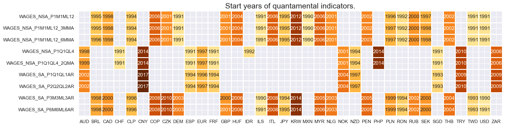
Availability

Available history of wage series is very uneven across countries. Even some developed countries’ series only begin in the 2000s. Older “predecessor” series may, over time, be used to extend history. For the explanation of currency symbols, which are related to currency areas or countries for which categories are available, please view Appendix 2 .

xcatx = main
cidx = cids

msm.check_availability(
    df,
    xcats=xcatx,
    cids=cidx,
    missing_recent=False,
)

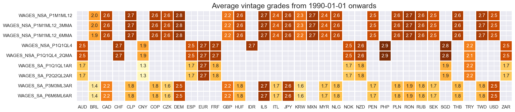
Easily available top-grade vintages rarely go back far in history.

xcatx = main
cidx = cids

plot = msp.heatmap_grades(
    df,
    xcats=xcatx,
    cids=cidx,
    size=(19, 4),
    title=f"Average vintage grades from {start_date} onwards",
)

# Renaming for graphs for ease of subsequent analysis

dfx = df.copy()

dict_repl = {
    "WAGES_NSA_P1Q1QL4_2QMA": "WAGES_NSA_P1M1ML12_6MMA",
    "WAGES_NSA_P1Q1QL4": "WAGES_NSA_P1M1ML12_3MMA",
    "WAGES_SA_P2Q2QL2AR": "WAGES_TREND_P6M6ML6AR",
    "WAGES_SA_P1Q1QL1AR": "WAGES_SA_P3M3ML3AR",
   
}
for key, value in dict_repl.items():
    dfx["xcat"] = dfx["xcat"].str.replace(key, value)

cidx = cids

msp.view_ranges(
    dfx,
    xcats=["WAGES_NSA_P1M1ML12_6MMA", "WAGES_NSA_P1M1ML12_3MMA"],
    cids=cidx,
    val="eop_lag",
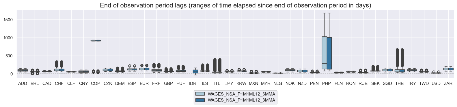
    title="End of observation period lags (ranges of time elapsed since end of observation period in days)",
    start="2000-01-01",
    kind="box",
    size=(16, 4),
)
msp.view_ranges(
    dfx,
    xcats=["WAGES_NSA_P1M1ML12_6MMA", "WAGES_NSA_P1M1ML12_3MMA"],
    cids=cidx,
    val="mop_lag",
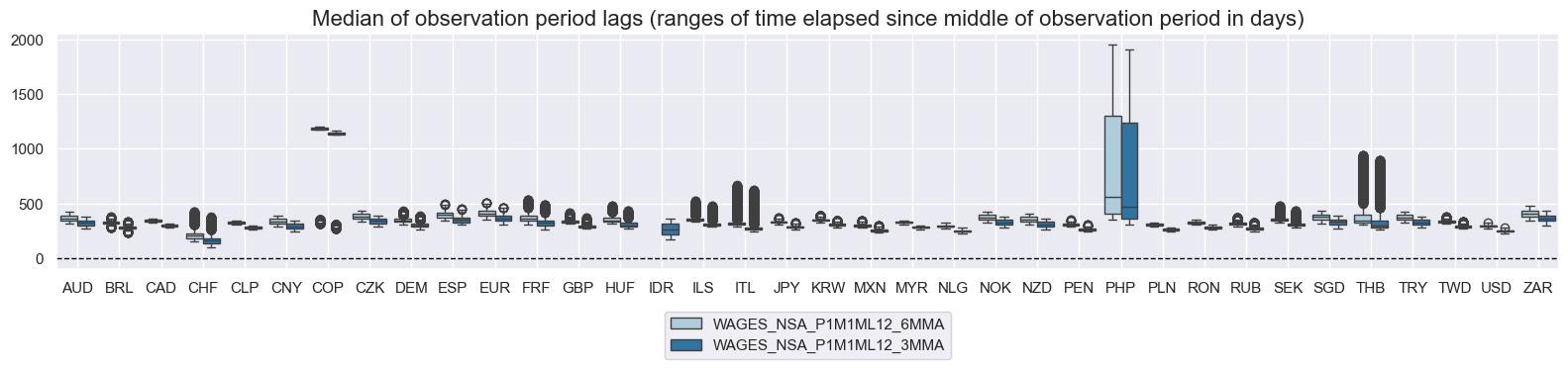
    title="Median of observation period lags (ranges of time elapsed since middle of observation period in days)",
    start="2000-01-01",
    kind="box",
    size=(16, 4),
)

History

Wage growth

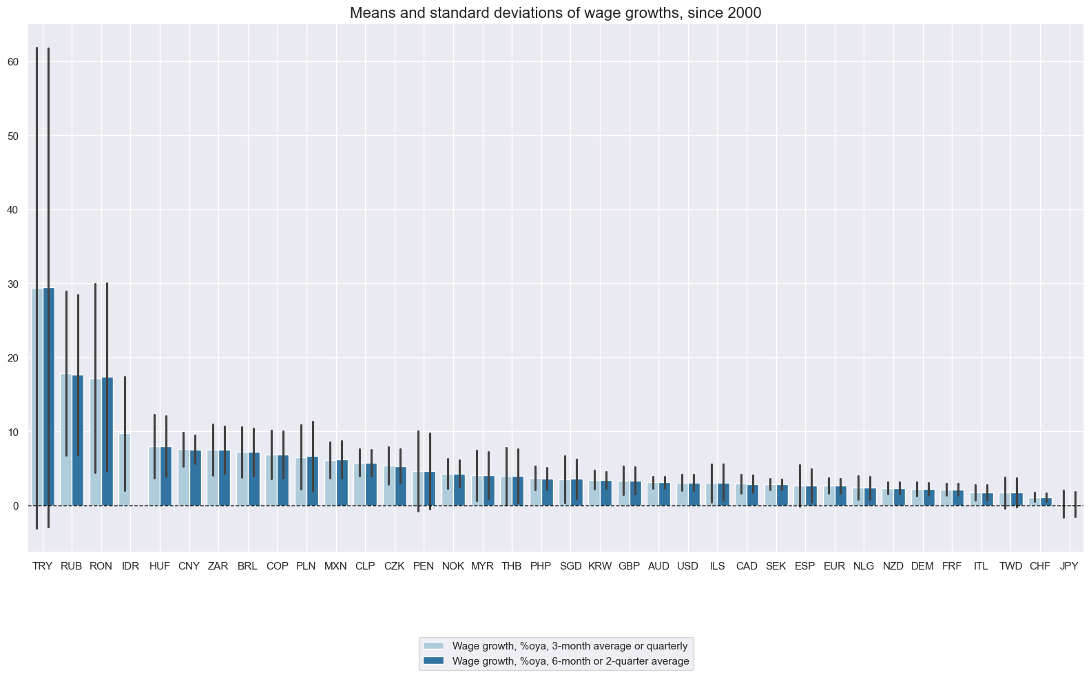
Wage growth rates and their standard deviations have been extremely uneven across countries. This reflects vast differences in both data quality and institutional background. It may not be easy to compare wage trends across countries in terms of their implication for monetary policy and competitiveness.

xcatx = ["WAGES_NSA_P1M1ML12_3MMA", "WAGES_NSA_P1M1ML12_6MMA"]
cidx = cids

msp.view_ranges(
    dfx,
    xcats=xcatx,
    cids=cidx,
    title="Means and standard deviations of wage growths, since 2000",
    xcat_labels=[
        "Wage growth, %oya, 3-month average or quarterly",
        "Wage growth, %oya, 6-month or 2-quarter average",
    ],
    sort_cids_by="mean",
    start="2000-01-01",
    kind="bar",
    size=(16, 10),
)

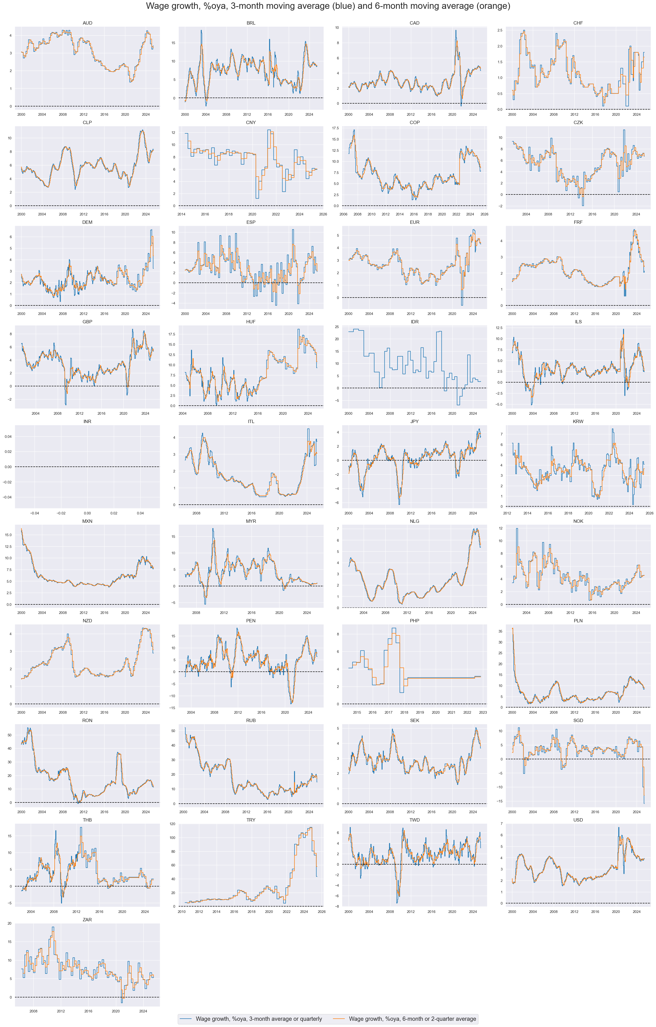
xcatx = ["WAGES_NSA_P1M1ML12_3MMA", "WAGES_NSA_P1M1ML12_6MMA"]
cidx = cids

msp.view_timelines(
    dfx,
    xcats=xcatx,
    cids=cidx,
    xcat_labels=[
        "Wage growth, %oya, 3-month average or quarterly",
        "Wage growth, %oya, 6-month or 2-quarter average",
    ],
    start="2000-01-01",
    title="Wage growth, %oya, 3-month moving average (blue) and 6-month moving average (orange)",
    title_fontsize=27,
    legend_fontsize=17,
    ncol=4,
    same_y=False,
    size=(20, 20),
    all_xticks=True,
)

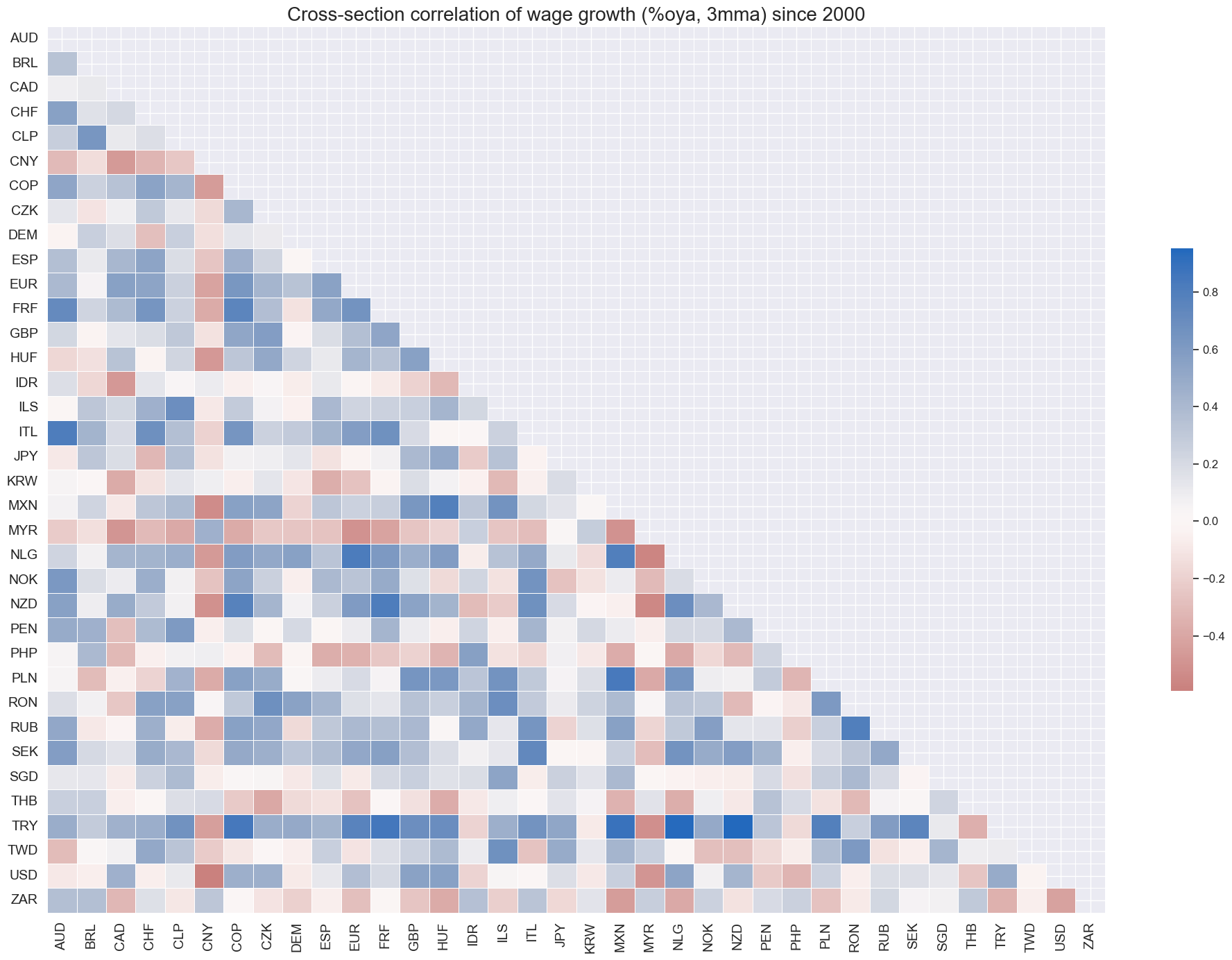
Quantamental metrics of wage growth have not generally been strongly correlated across countries.

cidx = list(set(cids) - set(["INR"]))
msp.correl_matrix(
    dfx,
    xcats="WAGES_NSA_P1M1ML12_3MMA",
    cids=cidx,
    title="Cross-section correlation of wage growth (%oya, 3mma) since 2000",
    size=(20, 14),
)

Short-term wage growth

Similar to wage growth, wage trends tend to be highly varied and uneven amongst countries.

xcatx = [   
"WAGES_SA_P3M3ML3AR","WAGES_SA_P6M6ML6AR", 
        ]
cidx = cids

msp.view_ranges(
    dfx,
    xcats=xcatx,
    cids=cidx,
    title="Means and standard deviations of wage trends, since 2000",
    xcat_labels=[
        "Wage trends, seasonally adjusted, % 3 months over 3 months, annualized",
        "Wage trends, seasonally adjusted, % 6 months over 6 months, annualized",
    ],
    sort_cids_by="mean",
    start="2000-01-01",
    kind="bar",
    size=(16, 10),
)

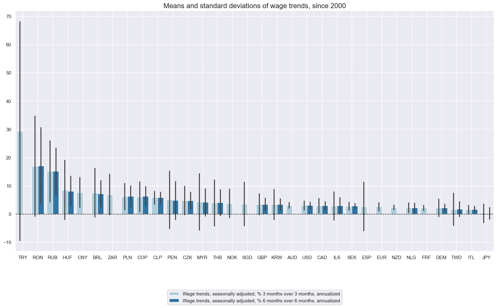
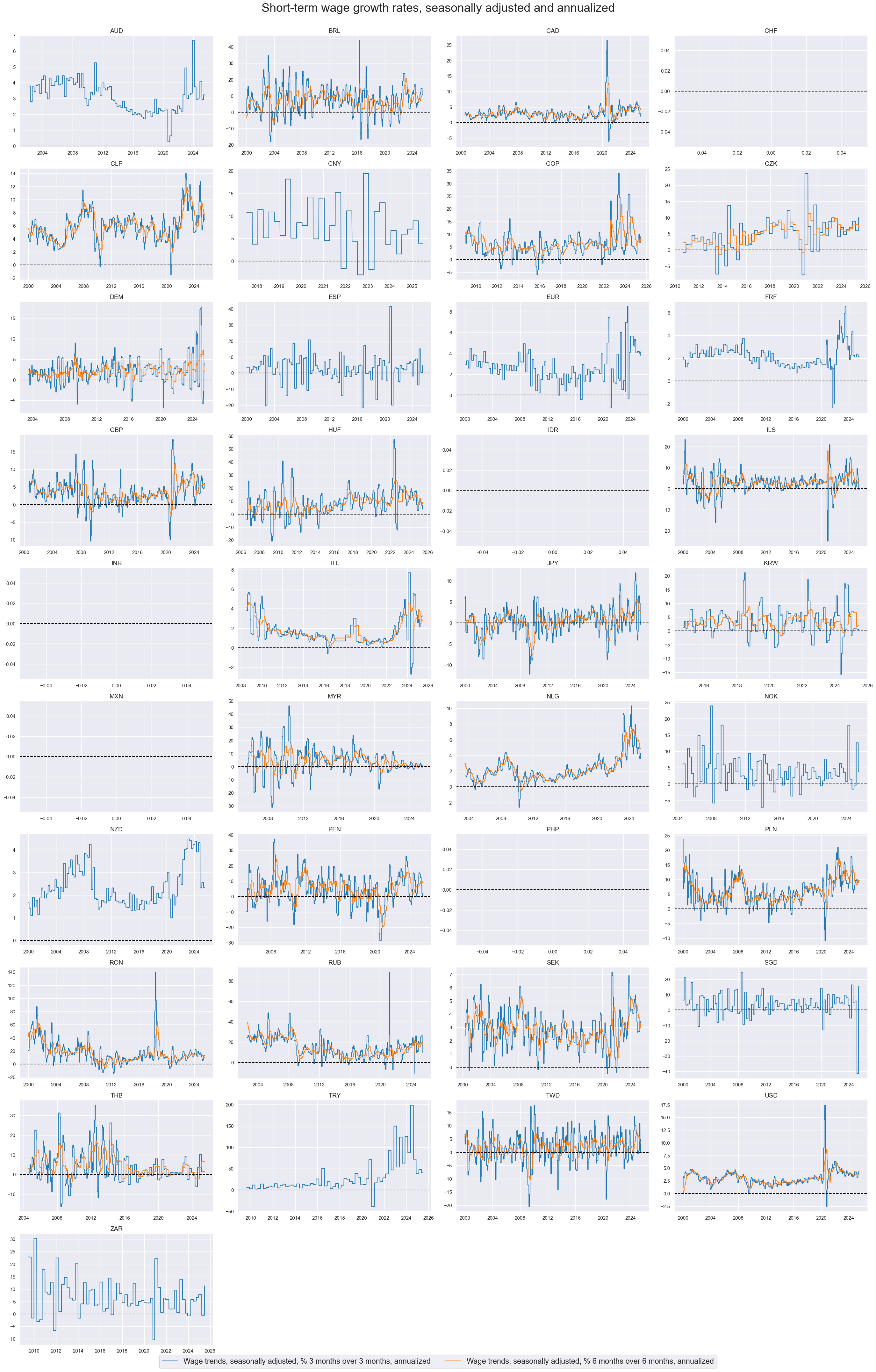
Quarterly or 3-month over 3-month trends are very volatile, but 6-month over 6-month trends often serve well as timely trend indicators.

xcatx = [   
"WAGES_SA_P3M3ML3AR","WAGES_SA_P6M6ML6AR", 
        ]
cidx = cids

msp.view_timelines(
    dfx,
    xcats=xcatx,
    cids=cidx,
    xcat_labels=[
        "Wage trends, seasonally adjusted, % 3 months over 3 months, annualized",
        "Wage trends, seasonally adjusted, % 6 months over 6 months, annualized",
    ],
    start="2000-01-01",
    title="Short-term wage growth rates, seasonally adjusted and annualized",
    title_fontsize=27,
    legend_fontsize=17,
    ncol=4,
    same_y=False,
    size=(20, 20),
    all_xticks=True,
)

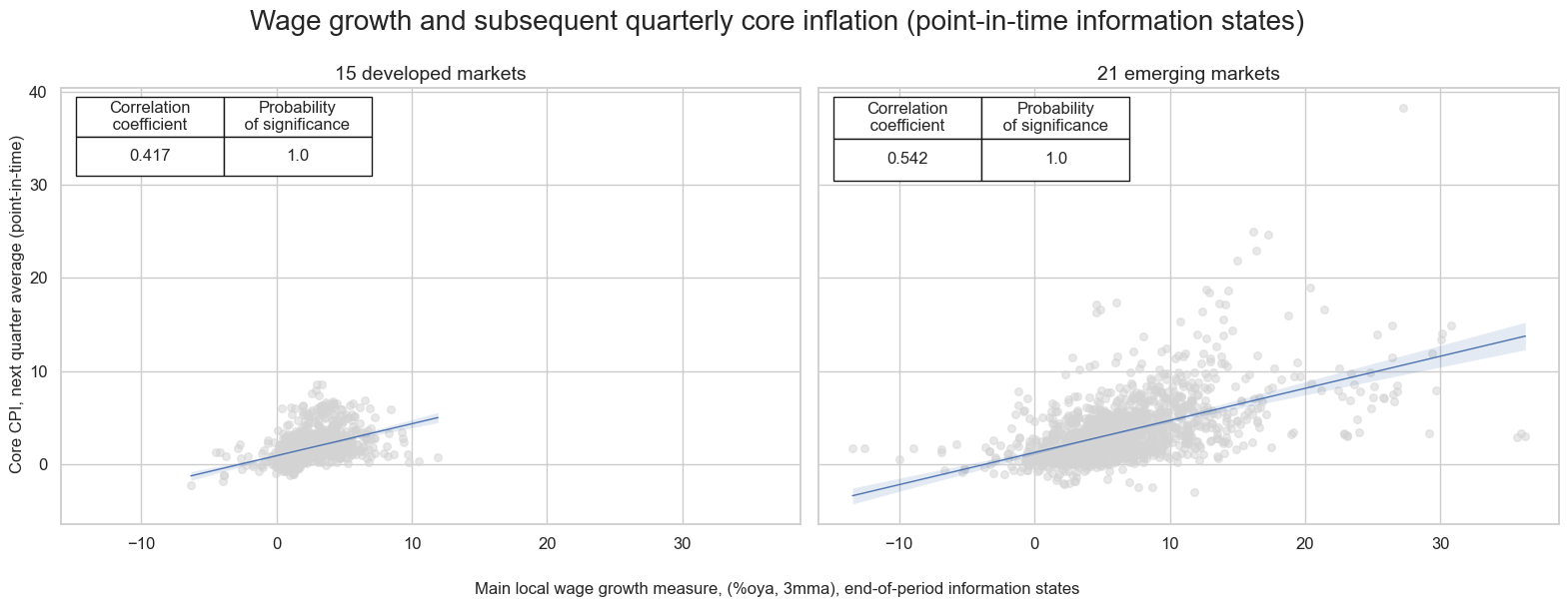
There has been a strong correlation between wage growth and subsequent core inflation in both developed and emerging markets.

cidx_infl = {
    "15 developed markets": cids_dm,  
    "21 emerging markets ": list(set(cids_em) - {'INR'}),  
}

cr = {}


for cid_name, cid_list in cidx_infl.items(): 
      cr[f"cr_{cid_name}"] = msp.CategoryRelations(
            dfx,
            xcats=["WAGES_NSA_P1M1ML12_3MMA", 'CPIC_SA_P1M1ML12'],
            cids=cid_list,
            freq="Q",
            lag=1,
            xcat_aggs=["last", "mean"],
            xcat_trims=[40,40], # for plot focus
            start="2000-01-01",
           
        )

#Combine all CategoryRelations instances for plotting
all_cr_instances = [
    cr[f"cr_{cid_name}"]
    for cid_name in cidx_infl.keys() 
]

# Dynamically create subplot titles based on identifiers and market types
subplot_titles = [
    f"{cid_name}"  # Use the descriptive keys from cidx directly
    for cid_name in cidx_infl.keys()
]

# plot side by side all the CategoryRelations instances
msv.multiple_reg_scatter(
        all_cr_instances,
        title="Wage growth and subsequent quarterly core inflation (point-in-time information states)" ,
        xlab="Main local wage growth measure, (%oya, 3mma), end-of-period information states",
        ylab="Core CPI, next quarter average (point-in-time)",
        ncol=2,
        nrow=1,
        figsize=(16, 6),
        prob_est="map",
        subplot_titles = subplot_titles,
        coef_box="upper left",
        
     )

Importance

Research links

“On a quarterly basis, risk aversion shocks explain roughly 75% of variation in the log difference of stock market wealth, but the near permanent factors share shocks plays an increasingly important role as the time horizon extends. We find that more than 100% of the increase since 1980 in the deterministically detrended log real value of the stock market, or a rise of 65% [in the stock market], is attributable to the cumulative effects of the factors share shock, which persistently redistributed rewards away from workers and toward shareholders over this period .” Greenwald, Lettau, and Ludvigson

“Researchers, at least since Mayers (1972), have long recognized the importance of accounting for labor income … in asset pricing tests.” Santos and Veronesi

on wage growth and fixed income returns

“… fluctuations in expected future labor income are a strong predictor of both real stock returns and excess returns over a Treasury bill rate…” C Julliard

on wage growth and equity returns

“… labor share is an important firm characteristic that generates cross-sectional variation in expected returns…” Donangelo, Gourio, Kehrig & Palacios

“… Our study highlights the important role of employee sentiment in stock market. We show that its negative return predictability is driven primarily by employees’ extrapolative bias. Employees are likely to extrapolate the most recent firm performance into the future and expect that firms will continue to perform well. This biased belief leads to immobility of employees in the labor market, increasing firms’ employment costs, such as wages. Consequently, the sentiment-driven cost lowers firms’ cash flows, resulting in a stock price reversal.” Chen, Tang, Yao & Zhou

“… expected future labor income growth rates and the residuals of the cointegration relation among log consumption, log asset wealth and log current labor income …, should help predict U.S. quarterly stock market returns and explain the cross-section of average returns.” C Julliard

Empirical clues

# Blacklist periods of FX targeting or illiquidity

dfb = dfx[dfx["xcat"].isin(["FXTARGETED_NSA", "FXUNTRADABLE_NSA"])].loc[
    :, ["cid", "xcat", "real_date", "value"]
]
dfba = (
    dfb.groupby(["cid", "real_date"])
    .aggregate(value=pd.NamedAgg(column="value", aggfunc="max"))
    .reset_index()
)
dfba["xcat"] = "FXBLACK"
fxblack = msp.make_blacklist(
    dfba, "FXBLACK"
)  # dictionary of periods of FX targeting or illiquidity

Wage growth and government bond returns

# Calculate logical excess trends and z-scores

calcs = [
    "RWAGES_NSA_P1M1ML12_3MMA = WAGES_NSA_P1M1ML12_3MMA - INFTARGET_NSA",  
    "RWAGES_NSA_P1M1ML12_6MMA = WAGES_NSA_P1M1ML12_6MMA - INFTARGET_NSA",
    "XWAGES_NSA_P1M1ML12_6MMA = WAGES_NSA_P1M1ML12_6MMA - ( RGDP_SA_P1Q1QL4_20QMM - WFORCE_NSA_P1Y1YL1_5YMM + INFTEFF_NSA )", # Excess wage growth
    
]

dfa = msp.panel_calculator(dfx, calcs, cids=cids)
dfx = msm.update_df(dfx, dfa)

alls = [
    "WAGES_NSA_P1M1ML12_3MMA",
    "RWAGES_NSA_P1M1ML12_3MMA", 
    "WAGES_NSA_P1M1ML12_6MMA",
    "XWAGES_NSA_P1M1ML12_6MMA",
    "RWAGES_NSA_P1M1ML12_6MMA",
]

dfa = pd.DataFrame(columns=dfx.columns)

# Z-scores for all series
for xc in alls:
    dfaa = msp.make_zn_scores(
        dfx,
        xcat=xc,
        cids=cids,
        sequential=True,
        min_obs=2 * 261,
        neutral="zero",
        pan_weight=1,
        thresh=3,
        postfix="_ZNW3",
        est_freq="M",
    )
    dfa = msm.update_df(dfa, dfaa)
dfx = msm.update_df(dfx, dfa)

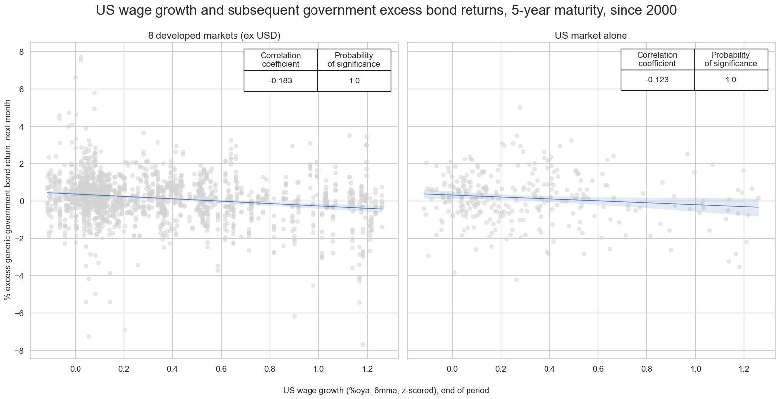
While wage growth data are not as keenly watched by bond markets as inflation data, their predictive power has been significant. There has been a negative relation between wage growth and subsequent government bond returns across developed countries. The relation was particularly strong and significant in the U.S., which not only hosts the the most important bond market but also reports wage data in a timely fashion. Moreover, U.S. wage growth exhibits a strong and significant correlation with subsequent bond returns in other developed markets on weekly, monthly and quarterly basis.

# add US wage growths to all cross-sections 

calcs = [
    "iUSD_WAGES_NSA_P1M1ML12_6MMA_ZNW3 = iUSD_WAGES_NSA_P1M1ML12_6MMA_ZNW3", 
    "iUSD_RWAGES_NSA_P1M1ML12_6MMA_ZNW3 = iUSD_RWAGES_NSA_P1M1ML12_6MMA_ZNW3", 
    "iUSD_XWAGES_NSA_P1M1ML12_6MMA_ZNW3 = iUSD_XWAGES_NSA_P1M1ML12_6MMA_ZNW3"]
    
dfa = msp.panel_calculator(dfx, calcs, cids=cids)
dfx = msm.update_df(dfx, dfa)

# specify the signals and targets for the analysis
sigx_gov = {
    "iUSD_RWAGES_NSA_P1M1ML12_6MMA_ZNW3": "US real smoothed wage growth (%oya, 6mma, z-scored, winsorized at 3SD)",
}

targx_gov = {
    "GB05YXR_NSA": "generic government bond excess returns: 5-year maturity"
}

# specify available currency areas
cidx_gov = msm.common_cids(dfx, xcats=list(sigx_gov.keys()) + list(targx_gov.keys()))

cidx_dict_gov = {
    f"{len(set(cidx_gov) - {'USD'})} developed markets (ex USD)": sorted(set(cidx_gov) - {"USD"}),  
    "US market alone": ["USD"],  
}


# Iterate through the mapped currency areas: 

cr = {}

for cid_name, cid_list in cidx_dict_gov.items(): 
      cr[f"cr_{cid_name}"] = msp.CategoryRelations(
            dfx,
            xcats=[", ".join(sigx_gov.keys()), ", ".join(targx_gov.keys())],
            cids=cid_list,
            freq="M",
            lag=1,
            xcat_aggs=["last", "sum"],
            blacklist=fxblack,
            start="2000-01-01",       
        )

#Combine all CategoryRelations instances for plotting
all_cr_instances = [
    cr[f"cr_{cid_name}"]
    for cid_name in cidx_dict_gov.keys() 
]

# Dynamically create subplot titles based on identifiers and market types
subplot_titles = [
    f"{cid_name}"  # Use the descriptive keys from cidx directly
    for cid_name in cidx_dict_gov.keys()
]

# plot side by side all the CategoryRelations instances
msv.multiple_reg_scatter(
        all_cr_instances,
        title="US wage growth and subsequent government excess bond returns, 5-year maturity, since 2000" ,
        xlab="US wage growth (%oya, 6mma, z-scored), end of period",
        ylab="% excess generic government bond return, next month",
        ncol=2,
        nrow=1,
        figsize=(16, 8),
        prob_est="map",
        subplot_titles = subplot_titles,
        coef_box="upper right",
        
     )

Wage growth as a predictor of IRS returns

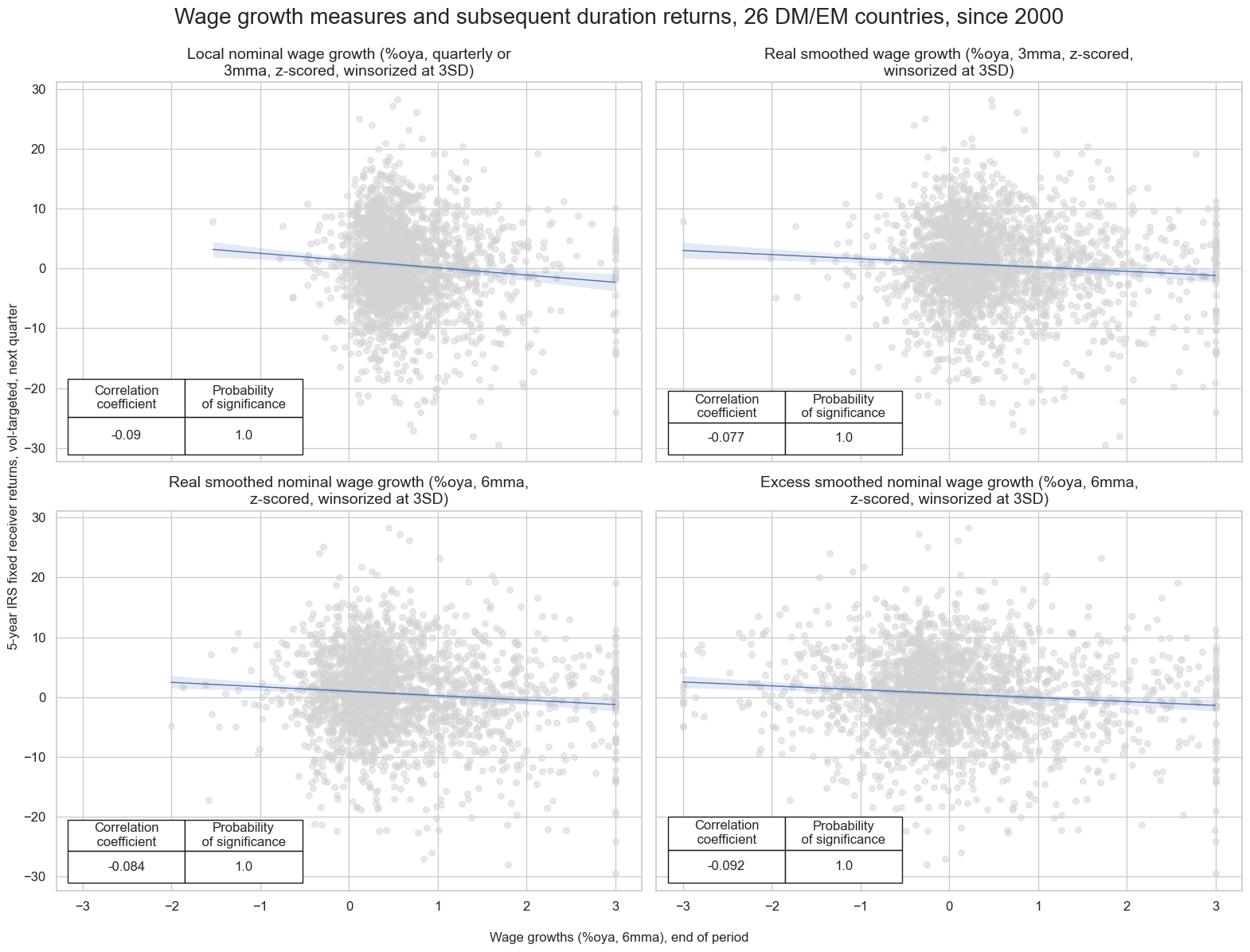
The has been pervasive evidence of predictive power of various measures of wage growth for duration returns, i.e. 5-year IRS fixed receiver returns, across developed and emerging countries. At a global scale the relation is negative and significant across time and countries. The predictive relation holds for monthly and quarterly frequency and both for simple and vol-targeted positions. The US indicators alone display significant predictive power duration returns in developed and emerging countries.

# specify the signals and targets for the analysis

sigx_irs = {
    "WAGES_NSA_P1M1ML12_3MMA_ZNW3": "Local nominal wage growth (%oya, quarterly or 3mma, z-scored, winsorized at 3SD)",
    "RWAGES_NSA_P1M1ML12_3MMA_ZNW3": "Real smoothed wage growth (%oya, 3mma, z-scored, winsorized at 3SD)",
    "RWAGES_NSA_P1M1ML12_6MMA_ZNW3": "Real smoothed nominal wage growth (%oya, 6mma, z-scored, winsorized at 3SD)",
    "XWAGES_NSA_P1M1ML12_6MMA_ZNW3": "Excess smoothed nominal wage growth (%oya, 6mma, z-scored, winsorized at 3SD)", 
}

sigx = [key for key in sigx_irs.keys()]

targx_irs = {
    "DU05YXR_VT10": "5-year IRS fixed receiver returns, vol-targeted at 10% a.r"
}

# specify available currency areas

cidx_irs = msm.common_cids(dfx, xcats=list(sigx_irs.keys()) + list(targx_irs.keys()))

cidx_dict_irs = {
    f"all {len(cidx_irs)} DM/EM markets": list(set(cidx_irs)),  
}

# Iterate through the mapped signals:
cr = {}

for sig in sigx: 
      cr[f"cr_{sig}"] = msp.CategoryRelations(
            dfx,
            xcats=[sig, ", ".join(targx_irs.keys())],
            cids=cidx_irs,
            freq="Q",
            lag=1,
            xcat_aggs=["last", "sum"],
            blacklist=fxblack,
            start="2000-01-01",
            xcat_trims=[30, 30] # for plot focus
        )
#Combine all CategoryRelations instances for plotting
all_cr_instances = [
    cr[f"cr_{sig}"]
    for sig in sigx_irs.keys()    
]

# create subplot titles based on identifiers and market types
subplot_titles = [lab for lab in list(sigx_irs.values())]


# plot side by side all the CategoryRelations instances
msv.multiple_reg_scatter(
        all_cr_instances,
        title=f"Wage growth measures and subsequent duration returns, {len(cidx_irs)} DM/EM countries, since 2000" ,
        xlab="Wage growths (%oya, 6mma), end of period",
        ylab="5-year IRS fixed receiver returns, vol-targeted, next quarter",
        ncol=2,
        nrow=2,
        figsize=(16, 12),
        prob_est="map",
        subplot_titles = subplot_titles,
        coef_box="lower left",
)

Wage growth as a predictor of equity index future returns

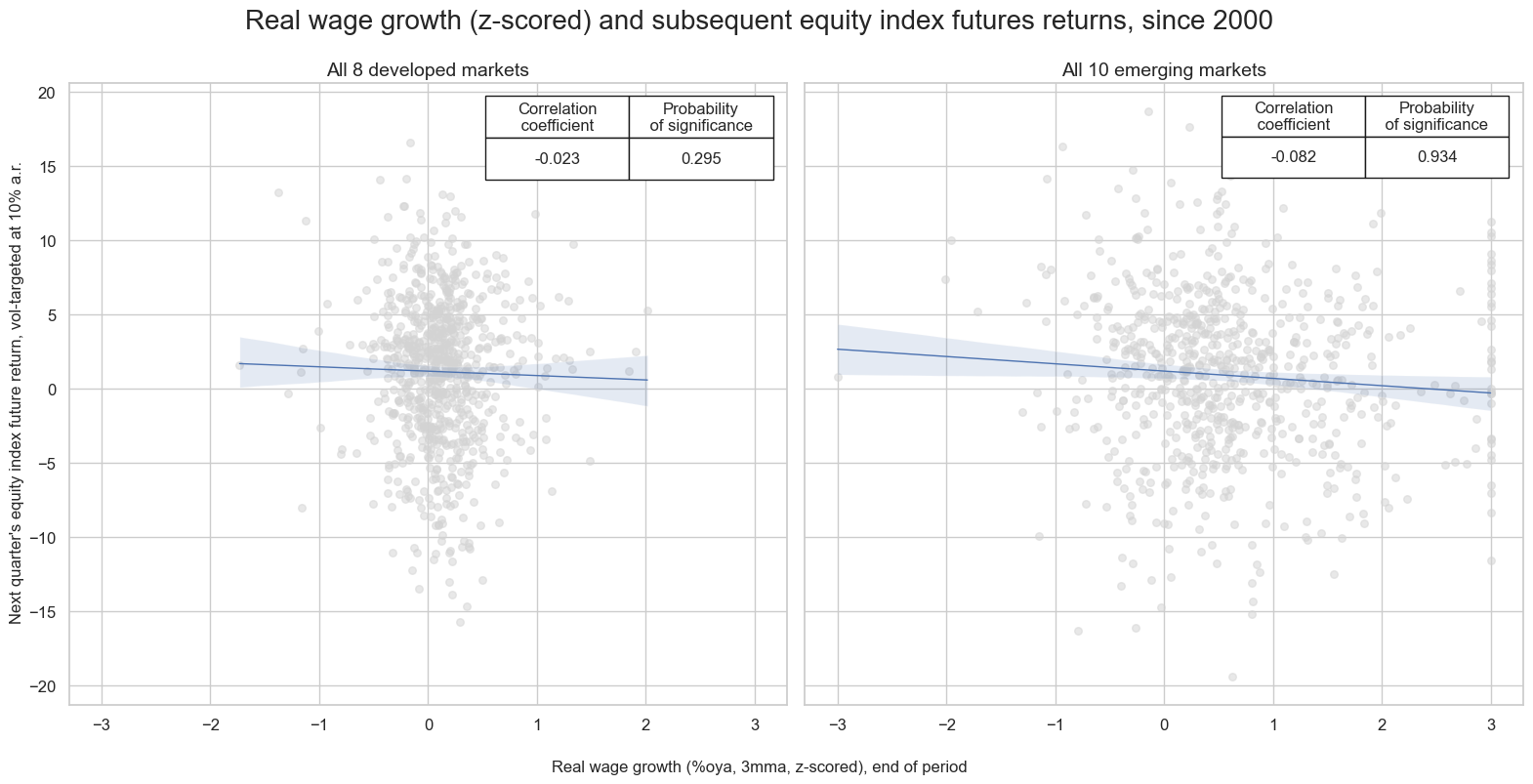
Wage growth that is substantially above the central bank’s inflation target should be a negative factor for equity returns because (a) it suggests a long-term reduction in profit margins and (b) it calls for tighter monetary policy.

Indeed, there has been a negative correlation between real wage growth (nominal wage growth minus the inflation target) and equity index future returns since 2000. However, the relation has only been significant for emerging markets.

# specify the signals and targets for the analysis

sigx_eq = {
    "RWAGES_NSA_P1M1ML12_3MMA_ZNW3": "Real smoothed wage growth (%oya, 3mma, z-scored, winsorized at 3SD)", 
}
sigx = [key for key in sigx_eq.keys()]

targx_eq = {
    "EQXR_VT10": "Equity index future return for 10% vol target",

}

# specify available currency areas
cidx_eq = msm.common_cids(dfx, xcats=list(sigx_eq.keys()) + list(targx_eq.keys()))

cidx_dict_eq = {
    f"All {len(set(cids_dmeq))} developed markets": list(set(cids_dmeq)),
    f"All {len(set(cids_emeq))} emerging markets": list(set(cids_emeq) )
}


# Iterate through the mapped currency areas: 
cr = {}


for cid_name, cid_list in cidx_dict_eq.items(): 
     
    cr[f"cr_{cid_name}"] = msp.CategoryRelations(
        dfx,
        xcats=[", ".join(sigx_eq.keys()), ", ".join(targx_eq.keys())],
        cids=cid_list,  
        freq="Q",
        lag=1,
        xcat_aggs=["last", "sum"],
        blacklist=fxblack,
        start="2000-01-01",
        
    )

#Combine all CategoryRelations instances for plotting
all_cr_instances = [
    cr[f"cr_{cid_name}"]
    for cid_name in cidx_dict_eq.keys() 
]

# Dynamically create subplot titles 
subplot_titles = [
    f"{cid_name}"  # Use the descriptive keys from cidx directly
    for cid_name in cidx_dict_eq.keys()
]

# plot side by side all the CategoryRelations instances
msv.multiple_reg_scatter(
        all_cr_instances,
        title="Real wage growth (z-scored) and subsequent equity index futures returns, since 2000" ,
        xlab="Real wage growth (%oya, 3mma, z-scored), end of period",
        ylab="Next quarter's equity index future return, vol-targeted at 10% a.r.",
        ncol=2,
        nrow=1,
        figsize=(16, 8),
        prob_est="map",
        subplot_titles = subplot_titles,
        coef_box="upper right",
   
     )

RWAGES_NSA_P1M1ML12_3MMA_ZNW3 misses: ['INR'].

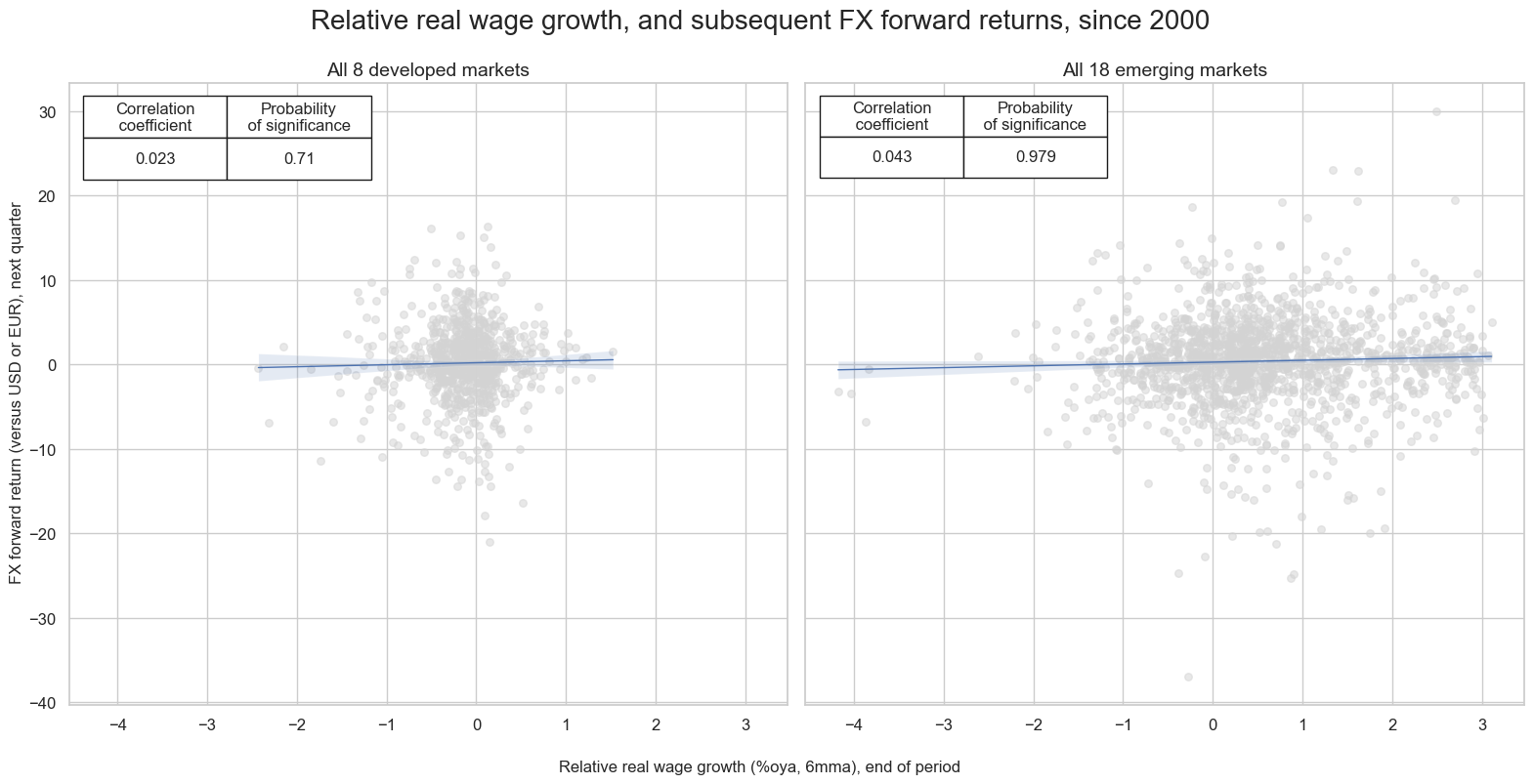
Relative wage growth as a predictor of FX returns

There is some evidence that relative real wage growth has positive predictive power for FX forward returns. The relation is particularly strong for emerging markets.

# Calculate relative values to benchmark currency areas

xcatx = ["RWAGES_NSA_P1M1ML12_6MMA_ZNW3"]

dfa_usd = msp.make_relative_value(dfx, xcatx, cids_usd, basket=["USD"], postfix="vBM")
dfa_eur = msp.make_relative_value(dfx, xcatx, cids_eur, basket=["EUR"], postfix="vBM")
dfa_eud = msp.make_relative_value(
    dfx, xcatx, cids_eud, basket=["EUR", "USD"], postfix="vBM"
)

dfa = pd.concat([dfa_eur, dfa_usd, dfa_eud])
dfx = msm.update_df(dfx, dfa)

# specify the signals and targets for the analysis
sigx_fx = {
        "RWAGES_NSA_P1M1ML12_6MMA_ZNW3vBM": "Real wage growth (%oya, 6mma, normalized) versus benchmark currency",
    } 

targx_fx = {
    "FXXR_NSA": "FX forward return: dominant cross"
}
cidx_fx = msm.common_cids(dfx, xcats=list(sigx_fx.keys()) + list(targx_fx.keys()))


cidx_dict_fx = {
   f"All {len(set(cids_dmfx) & set(cidx_fx))} developed markets": list(set(cids_dmfx) & set(cidx_fx)),  
   f"All {len(set(cids_emfx) & set(cidx_fx))} emerging markets": list(set(cids_emfx) & set(cidx_fx)), 
}

# Iterate through the mapped currency areas: 
cr = {}

for cid_name, cid_list in cidx_dict_fx.items(): 
     
    cr[f"cr_{cid_name}"] = msp.CategoryRelations(
        dfx,
        xcats=[", ".join(sigx_fx.keys()), ", ".join(targx_fx.keys())],
        cids=cid_list,  
        freq="q",
        lag=1,
        xcat_aggs=["last", "sum"],
        blacklist=fxblack,
        start="2000-01-01",
        xcat_trims=[50, 50] # for focus
    )

# Combine all CategoryRelations instances for plotting
all_cr_instances = [
    cr[f"cr_{cid_name}"]
    for cid_name in cidx_dict_fx.keys()
]

# Dynamically create subplot titles 
subplot_titles = [
    f"{cid_name}"  # Use the descriptive keys from cidx directly
    for cid_name in cidx_dict_fx.keys()
]

# plot side by side all the CategoryRelations instances
msv.multiple_reg_scatter(
    all_cr_instances,
    title="Relative real wage growth, and subsequent FX forward returns, since 2000",
    xlab="Relative real wage growth (%oya, 6mma), end of period",
    ylab="FX forward return (versus USD or EUR), next quarter",
    ncol=2,
    nrow=1,
    figsize=(16, 8),
    prob_est="map",
    coef_box="upper left",
    subplot_titles=subplot_titles,
    )

Appendices

Appendix 1: Country-specific notes

Further notes on wage data, for each cross-section are as below:

• AUD: In Australia, wages are post income tax and exclude bonuses.

• BRL: For Brazil, we use data on pre-tax wages from the main job.

• CAD: For Canada, we use a composite of hourly and weekly earnings growth. Both are after tax earnings and excluded agriculture.

• CLP: Chilean wage data are before income tax.

• CNY: China wages data are after income tax.

• COP: Colombian wage data are before income tax.

• CZK: Czech data encompass the following sectors: industry, market services, construction, and agriculture.

• DEM: For Germany, we use two wage series including bonuses and affter tax, from the Bundesbank and the statistics office.

• ESP: For Spain, we use salaries before taxes.

• FRF: For France, we use monthly non-farm average wages.

• EUR: For the euro area, we use a composite of OECD and eurostat data, both of which are after taxes.

• GBP: UK data are wages after taxes.

• HUF: Hungarian wage growth uses a composite of pre and post income tax wage data with and without tax benefits.

• ILS: For Israel, we use a composite of national bank and statistics office data.

• ITL: For Italy, we use wages including bonuses and before taxes.

• JPY: Japan wage data before taxes and a composite of cabinet office and statistics office data.

• KRW: In order to account for the impact of the lunar new year on South Korea (bonus payments), January and Feburary observations are combined and assigned to the release date for February.

• MXN: In Mexico, wage data are after taxes and exclude bonuses and growth is composite based on contractual wages and daily earnings.

• NLG: For the Netherlands, we use two wage series, one with and one without bonuses.

• NOK: For Norway, data are before income tax exclude bonuses. Also, prior to 2016 the series is based on manufacturing wages, rather than economy-wide wages.

• NZD: For New Zealand, we use a salary and wage index that excludes performance-based pay and is after income tax.

• PEN: For Peru, we actually use a time series of average income in Lima.

• PHP: The Philipines stopped reporting wage data in 2018.

• PLN: For Poland, we use average monthly wages before taxes.

• RON: For Romania, we use an average monthly wage series that includes bonuses and is before taxes.

• RUB: For Russia, the series measures average monthly wages, includes bonuses and is before taxes.

• SEK: For Sweden, we use average monthly wages and salaries combining data of the national mediation office and and the statistics office.

• SGD: For Singapore, we refer to average monthly income after taxes.

• THB: The Thai wage growth series is based on a composite of average wages as published by the national bank and the statistics office.

• TRY: For Turkey, we use total hourly earnings before taxes.

• TWD: For Taiwan, we look at average monthly earnings including bonuses and after taxes. In order to account for the impact of the lunar new year on Taiwan (bonus payments), January and Feburary observartions are combined and assigned to the release date for February.

• USD: The U.S. wage growth series is based on an average of average weekly and hourly earnings and refers only to private employees.

• ZAR: For South Africa, we use average monthly earnings after taxes and including bonuses.

Appendix 2: Currency symbols

The word ‘cross-section’ refers to currencies, currency areas or economic areas. In alphabetical order, these are AUD (Australian dollar), BRL (Brazilian real), CAD (Canadian dollar), CHF (Swiss franc), CLP (Chilean peso), CNY (Chinese yuan renminbi), COP (Colombian peso), CZK (Czech Republic koruna), DEM (German mark), ESP (Spanish peseta), EUR (Euro), FRF (French franc), GBP (British pound), HKD (Hong Kong dollar), HUF (Hungarian forint), IDR (Indonesian rupiah), ITL (Italian lira), JPY (Japanese yen), KRW (Korean won), MXN (Mexican peso), MYR (Malaysian ringgit), NLG (Dutch guilder), NOK (Norwegian krone), NZD (New Zealand dollar), PEN (Peruvian sol), PHP (Phillipine peso), PLN (Polish zloty), RON (Romanian leu), RUB (Russian ruble), SEK (Swedish krona), SGD (Singaporean dollar), THB (Thai baht), TRY (Turkish lira), TWD (Taiwanese dollar), USD (U.S. dollar), ZAR (South African rand).