Labor market tightness #
This category group contains point-in-time measures of latest available information on tightness or slack of labor markets. At present, it contains unemployment rates and unemployment gaps (i.e. unemployment rates in relation to multi-year averages, which form simple model-free reference values for natural unemployment). The state of the labor market is often regarded as a lagging indicator of business cycles, but an important factor of wage and price pressure, and monetary policy.
Unemployment rate #
Ticker : UNEMPLRATE_SA_3MMA
Label : Unemployment rate, sa, 3mma
Definition : Unemployment rate, seasonally adjusted, 3-month moving average
Notes :
-
Unemployment data are taken only from official statistics, not job agencies or surveys.
-
Most countries release monthly-frequency data with fairly short publication lags. However, Norway (NOK) only releases unemployment data quarterly.
-
The UK (GBP) and Peru (PEN) only release unemployment data in 3-month moving averages. However, these are updated at a monthly frequency.
Unemployment gaps #
Ticker : UNEMPLRATE_SA_3MMAv5YMA / _3MMAv10YMA / _3MMAv5YMM / _3MMAv10YMM
Label : Unemployment rate: 3mma vs 5yma / 3mma vs 10yma / 3mma vs 5ymm / 3mma vs 10ymm
Definition : Unemployment rate, seasonally adjusted: 3-month moving average minus the 5-year moving average / 3-month moving average minus the 10-year moving average / 3-month moving average minus the 5-year moving median / 3-month moving average minus the 10-year moving median
Notes :
-
Unemployment data are taken only from official statistics, not job agencies or surveys.
-
Most countries release monthly-frequency data with fairly short publication lags. However, Norway (NOK) only releases unemployment data quarterly.
-
The UK (GBP) and Peru (PEN) only release unemployment data in 3-month moving averages. However, these are updated at a monthly frequency.
Imports #
Only the standard Python data science packages and the specialized
macrosynergy
package are needed.
import os
import numpy as np
import pandas as pd
import matplotlib.pyplot as plt
import seaborn as sns
import math

import json
import yaml

import macrosynergy.management as msm
import macrosynergy.panel as msp
import macrosynergy.signal as mss
import macrosynergy.pnl as msn

from macrosynergy.download import JPMaQSDownload

from timeit import default_timer as timer
from datetime import timedelta, date, datetime

import warnings

warnings.simplefilter("ignore")
The
JPMaQS
indicators we consider are downloaded using the J.P. Morgan Dataquery API interface within the
macrosynergy
package. This is done by specifying
ticker strings
, formed by appending an indicator category code
<category>
to a currency area code
<cross_section>
. These constitute the main part of a full quantamental indicator ticker, taking the form
DB(JPMAQS,<cross_section>_<category>,<info>)
, where
<info>
denotes the time series of information for the given cross-section and category.
The following types of information are available:
-
valuegiving the latest available values for the indicator -
eop_lagreferring to days elapsed since the end of the observation period -
mop_lagreferring to the number of days elapsed since the mean observation period -
gradedenoting a grade of the observation, giving a metric of real time information quality.
After instantiating the
JPMaQSDownload
class within the
macrosynergy.download
module, one can use the
            download(tickers,


            start_date,


            metrics)
method to obtain the data. Here
tickers
is an array of ticker strings,
start_date
is the first release date to be considered and
metrics
denotes the types of information requested.
# Cross-sections of interest

cids_dmca = [
    "AUD",
    "CAD",
    "CHF",
    "EUR",
    "GBP",
    "JPY",
    "NOK",
    "NZD",
    "SEK",
    "USD",
]  # DM currency areas
cids_dmec = ["DEM", "ESP", "FRF", "ITL", "NLG"]  # DM euro area countries
cids_latm = ["BRL", "COP", "CLP", "MXN", "PEN"]  # Latam countries
cids_emea = ["CZK", "HUF", "ILS", "PLN", "RON", "RUB", "TRY", "ZAR"]  # EMEA countries
cids_emas = [
    "CNY",
    # "HKD",
    "IDR",
    "INR",
    "KRW",
    "MYR",
    "PHP",
    "SGD",
    "THB",
    "TWD",
]  # EM Asia countries

cids_dm = cids_dmca + cids_dmec
cids_em = cids_latm + cids_emea + cids_emas

cids = sorted(cids_dm + cids_em)
# Quantamental categories of interest

main = [
    "UNEMPLRATE_SA_3MMA",
    "UNEMPLRATE_SA_3MMAv5YMA",
    "UNEMPLRATE_SA_3MMAv10YMA",
    "UNEMPLRATE_SA_3MMAv5YMM",
    "UNEMPLRATE_SA_3MMAv10YMM",
]
econ = ["INTRGDP_NSA_P1M1ML12_3MMA", "IMPORTS_SA_P1M1ML12_3MMA"]  # economic context
mark = [
    "FXXR_NSA",
    "FXXR_VT10",
    "EQXR_NSA",
    "EQXR_VT10",
    "DU05YXR_NSA",
    "DU05YXR_VT10",
    "FXTARGETED_NSA",
    "FXUNTRADABLE_NSA",
    "FXXRHvGDRB_NSA",
]  # market links

xcats = main + econ + mark
# Download series from J.P. Morgan DataQuery by tickers

start_date = "2000-01-01"
tickers = [cid + "_" + xcat for cid in cids for xcat in xcats]
print(f"Maximum number of tickers is {len(tickers)}")

# Retrieve credentials

client_id: str = os.getenv("DQ_CLIENT_ID")
client_secret: str = os.getenv("DQ_CLIENT_SECRET")

# Download from DataQuery

with JPMaQSDownload(client_id=client_id, client_secret=client_secret) as downloader:
    start = timer()
    df = downloader.download(
        tickers=tickers,
        start_date=start_date,
        metrics=["value", "eop_lag", "mop_lag", "grading"],
        suppress_warning=True,
    )
    end = timer()

dfd = df

print("Download time from DQ: " + str(timedelta(seconds=end - start)))
Maximum number of tickers is 592
Downloading data from JPMaQS.
Timestamp UTC:  2025-05-06 08:54:04
Connection successful!
Some expressions are missing from the downloaded data. Check logger output for complete list.
340 out of 2368 expressions are missing. To download the catalogue of all available expressions and filter the unavailable expressions, set `get_catalogue=True` in the call to `JPMaQSDownload.download()`.
Some dates are missing from the downloaded data.
2 out of 6614 dates are missing.
Download time from DQ: 0:03:47.283917
Availability #
cids_not_exp = ["INR", "IDR", "CNY"]
cids_exp = sorted(
    list(set(cids) - set(cids_not_exp))
)  # cids expected in category panels
msm.missing_in_df(dfd, xcats=main, cids=cids_exp)
No missing XCATs across DataFrame.
Missing cids for UNEMPLRATE_SA_3MMA:        []
Missing cids for UNEMPLRATE_SA_3MMAv10YMA:  []
Missing cids for UNEMPLRATE_SA_3MMAv10YMM:  []
Missing cids for UNEMPLRATE_SA_3MMAv5YMA:   []
Missing cids for UNEMPLRATE_SA_3MMAv5YMM:   []
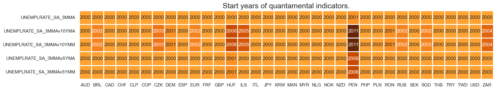
Real-time quantamental indicators of labour market tightness are available by the 2000s for most developed countries and many emerging economies. Peru is a notable late starter.
For the explanation of currency symbols, which are related to currency areas or countries for which categories are available, please view Appendix 1 .
xcatx = main
cidx = cids_exp

dfx = msm.reduce_df(dfd, xcats=xcatx, cids=cidx)
dfs = msm.check_startyears(dfx)
msm.visual_paneldates(dfs, size=(18, 3))

print("Last updated:", date.today())
Last updated: 2025-05-06
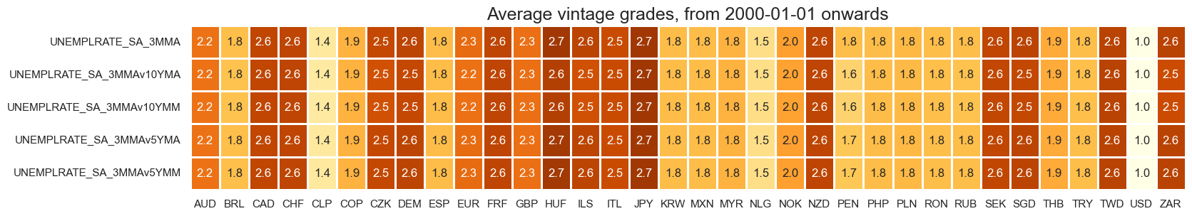
Vintage grading is mixed, with Chile the only country with high grade vintages consistently available across indicators.
plot = msp.heatmap_grades(
    dfd,
    xcats=xcatx,
    cids=cidx,
    start=start_date,
    size=(18, 3),
    title=f"Average vintage grades, from {start_date} onwards",
)
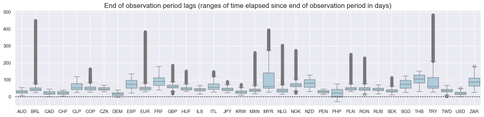
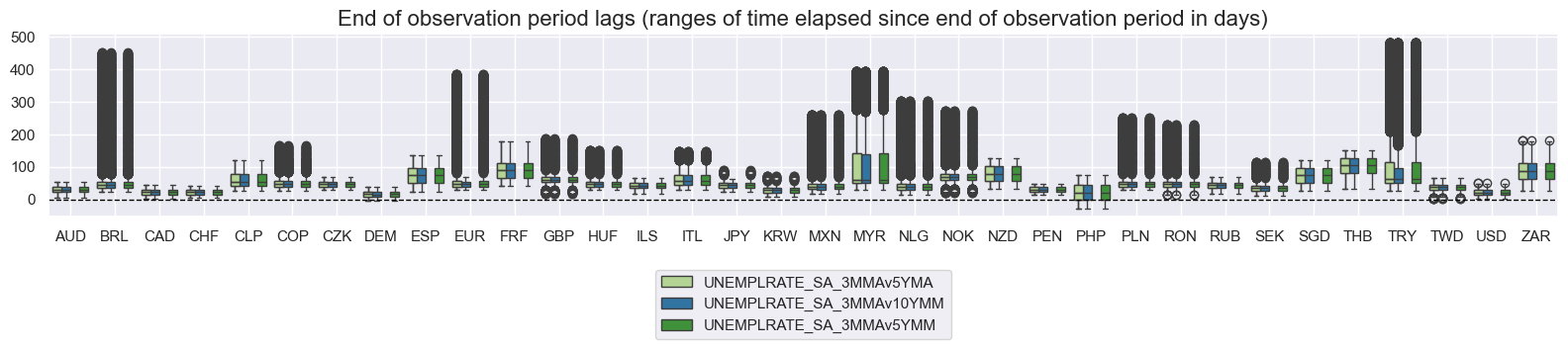
msp.view_ranges(
dfd,
xcats=["UNEMPLRATE_SA_3MMA"],
cids=cids_exp,
val="eop_lag",
title="End of observation period lags (ranges of time elapsed since end of observation period in days)",
start="2000-01-01",
kind="box",
size=(16, 4),
)
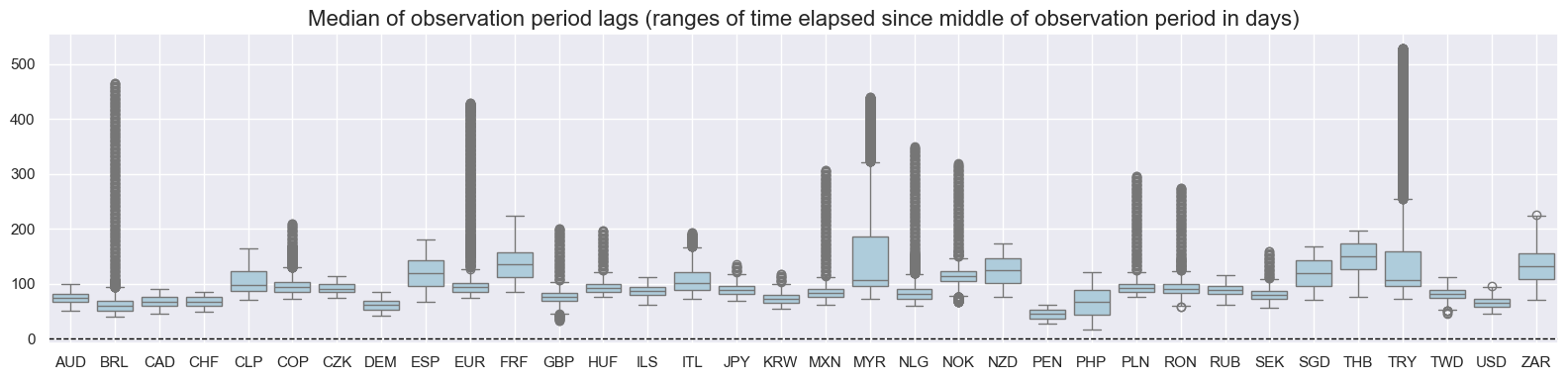
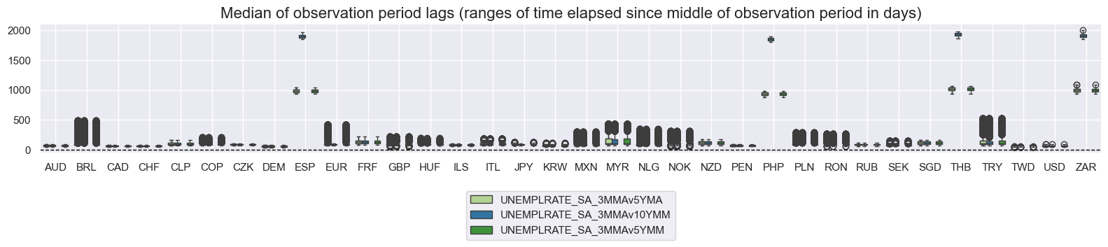
msp.view_ranges(
dfd,
xcats=["UNEMPLRATE_SA_3MMA"],
cids=cids_exp,
val="mop_lag",
title="Median of observation period lags (ranges of time elapsed since middle of observation period in days)",
start="2000-01-01",
kind="box",
size=(16, 4),
)
xcatx = [
    "UNEMPLRATE_SA_3MMAv5YMA",
    "UNEMPLRATE_SA_3MMAv10YMM",
    "UNEMPLRATE_SA_3MMAv5YMA",
    "UNEMPLRATE_SA_3MMAv5YMM",
]

msp.view_ranges(
    dfd,
    xcats=xcatx,
    cids=cids_exp,
    val="eop_lag",
    title="End of observation period lags (ranges of time elapsed since end of observation period in days)",
    start="2000-01-01",
    kind="box",
    size=(16, 4),
)
msp.view_ranges(
    dfd,
    xcats=xcatx,
    cids=cids_exp,
    val="mop_lag",
    title="Median of observation period lags (ranges of time elapsed since middle of observation period in days)",
    start="2000-01-01",
    kind="box",
    size=(16, 4),
)
History #
Unemployment rate #
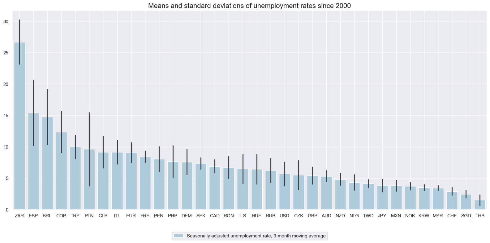
Long-term averages are vastly different across countries, reflecting differences in labor market structure, data collection, and social security. Countries with regulated labor markets and comprehensive unemployment benefits tend to have higher long-term unemployment rates.
xcatx = ["UNEMPLRATE_SA_3MMA"]
cidx = cids_exp

msp.view_ranges(
    dfd,
    xcats=xcatx,
    cids=cidx,
    sort_cids_by="mean",
    start=start_date,
    title="Means and standard deviations of unemployment rates since 2000",
    xcat_labels=["Seasonally adjusted unemployment rate, 3-month moving average"],
)
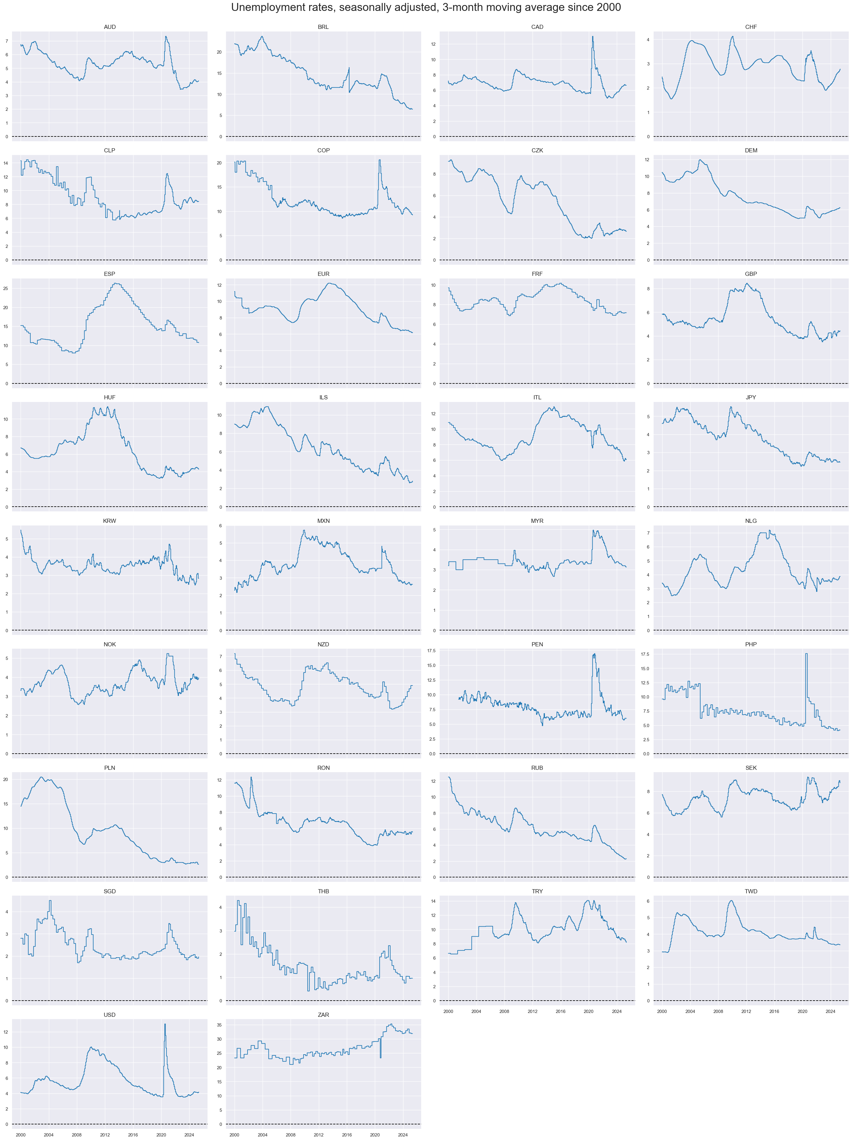
Unemployment trends have displayed long cycles and their 3-month moving averages show much less short-term volatility than comparable production indices.
xcatx = ["UNEMPLRATE_SA_3MMA"]
cidx = cids_exp

msp.view_timelines(
    dfd,
    xcats=xcatx,
    cids=cidx,
    start=start_date,
    title="Unemployment rates, seasonally adjusted, 3-month moving average since 2000",
    title_fontsize=27,
    ncol=4,
    same_y=False,
    size=(12, 7),
    aspect=1.7,
    all_xticks=False,
)
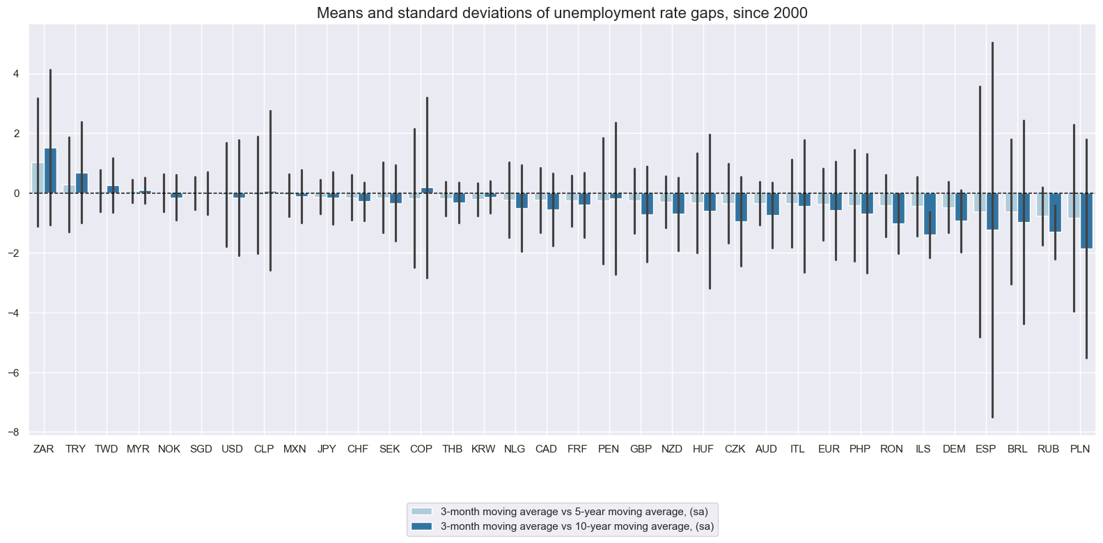
Unemployment rate gaps versus 5-10 year averages #
Focusing on differences between unemployment rates and multi-year averages naturally removes structural differences in recorded means. These gaps do not only capture the state of unemployment, but are also affected by any long-term secular trend. Economies with economic system transformation, such as in central and eastern Europe, have posted significant secular declines in joblessness in past decades.
xcatx = ["UNEMPLRATE_SA_3MMAv5YMA", "UNEMPLRATE_SA_3MMAv10YMA"]
cidx = cids_exp

msp.view_ranges(
    dfd,
    xcats=xcatx,
    cids=cidx,
    sort_cids_by="mean",
    start=start_date,
    title="Means and standard deviations of unemployment rate gaps, since 2000",
    xcat_labels=[
        "3-month moving average vs 5-year moving average, (sa)",
        "3-month moving average vs 10-year moving average, (sa)",
    ],
    kind="bar",
    size=(16, 8),
)
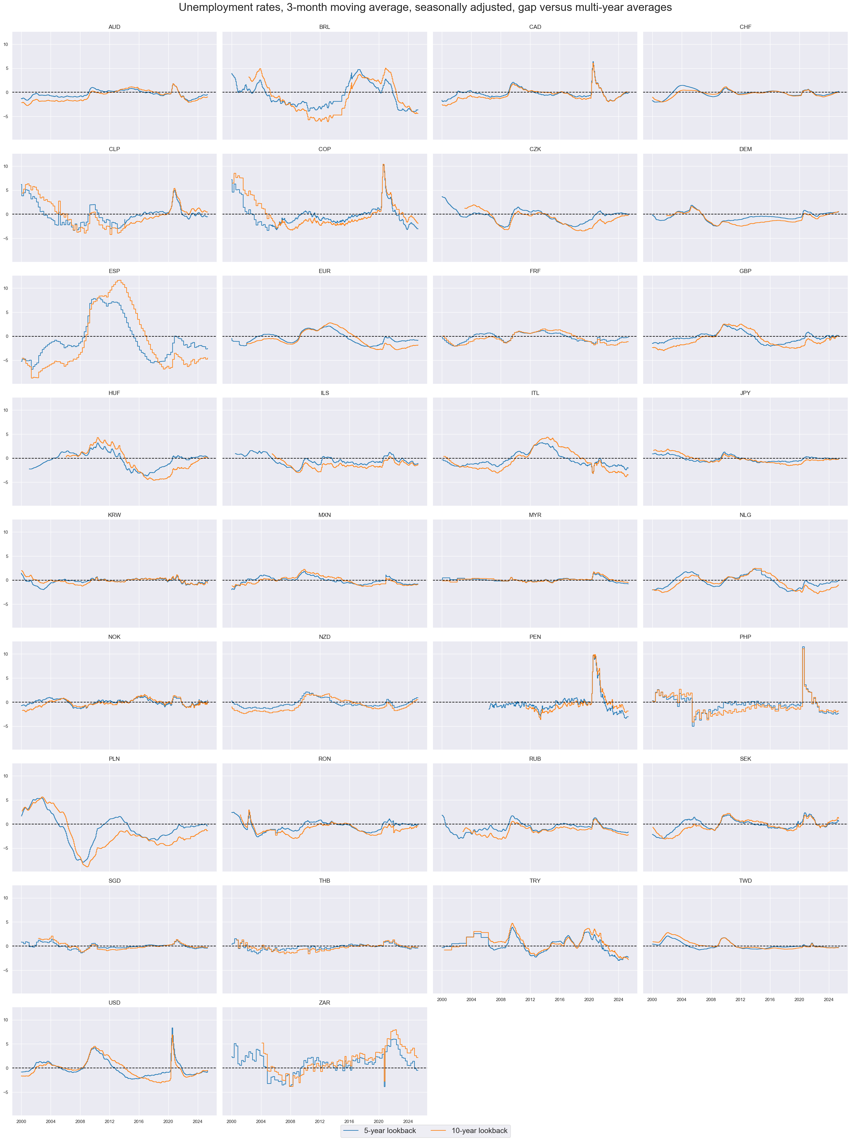
Unemployment gaps follow broad long-term business cycles.
xcatx = ["UNEMPLRATE_SA_3MMAv5YMA", "UNEMPLRATE_SA_3MMAv10YMA"]
cidx = cids_exp

msp.view_timelines(
    dfd,
    xcats=xcatx,
    cids=cidx,
    start=start_date,
    title="Unemployment rates, 3-month moving average, seasonally adjusted, gap versus multi-year averages",
    xcat_labels=["5-year lookback", "10-year lookback"],
    legend_fontsize=18,
    title_fontsize=27,
    ncol=4,
    same_y=True,
    size=(12, 7),
    aspect=1.7,
    all_xticks=False,
)
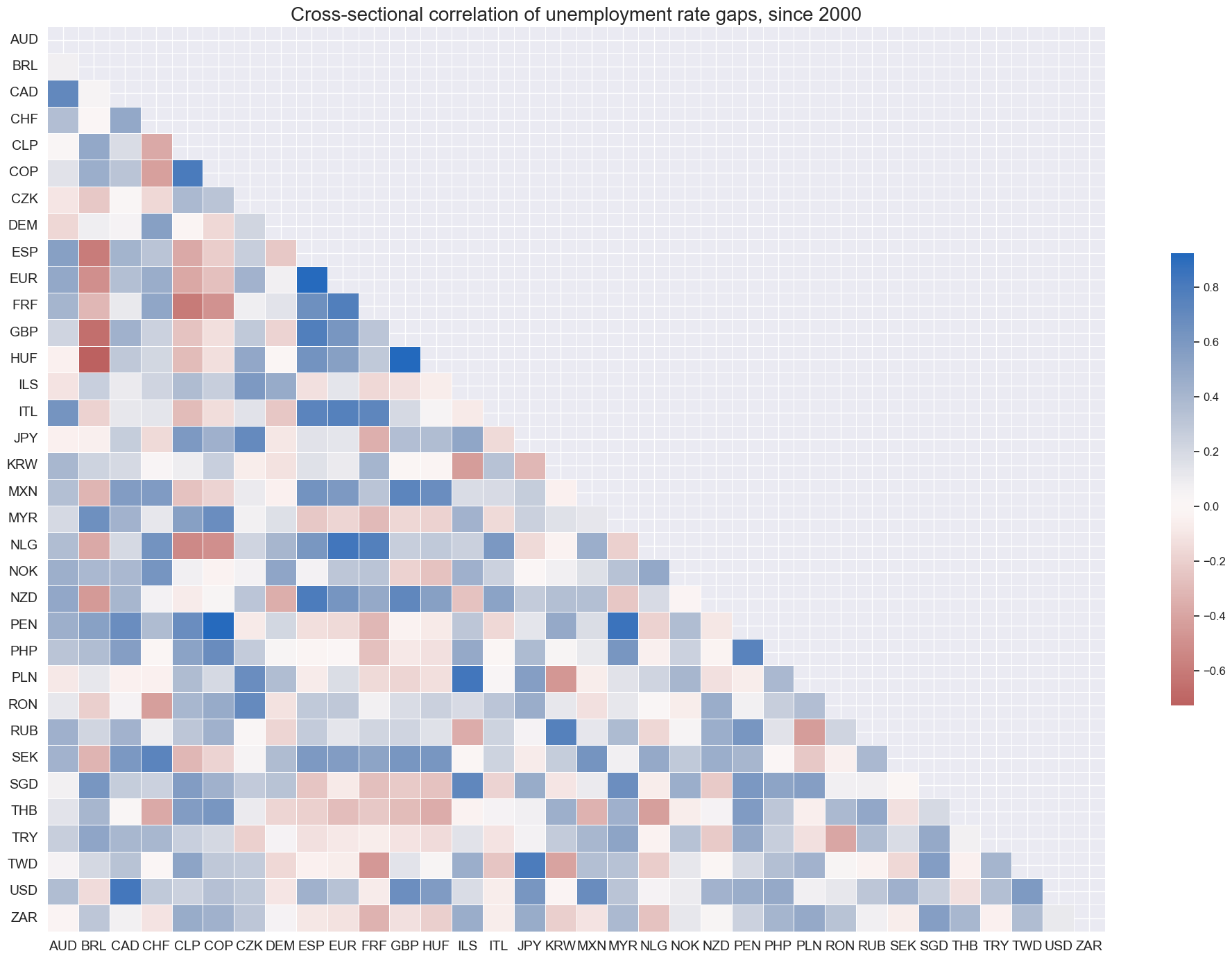
Interestingly, unemployment gaps, unlike economic growth trends, are not strongly positively correlated across countries. This plausibly reflects their greater dependence on domestic services and the different structure of labor markets, some of which require long notice periods for employment reductions.
cidx = cids_exp
msp.correl_matrix(
    dfd,
    xcats="UNEMPLRATE_SA_3MMAv5YMA",
    cids=cidx,
    size=(20, 14),
    start=start_date,
    title="Cross-sectional correlation of unemployment rate gaps, since 2000",
)
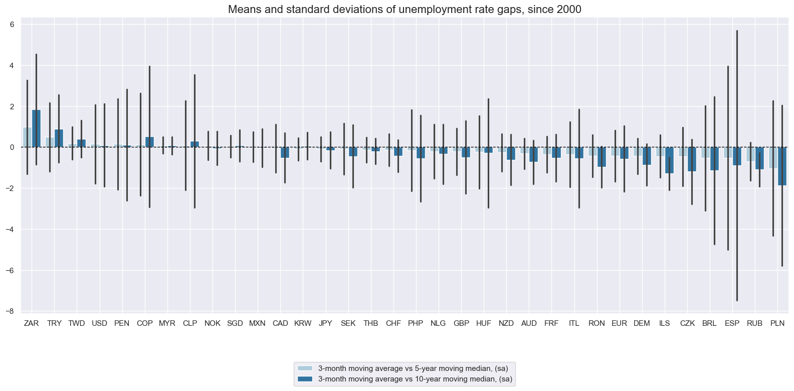
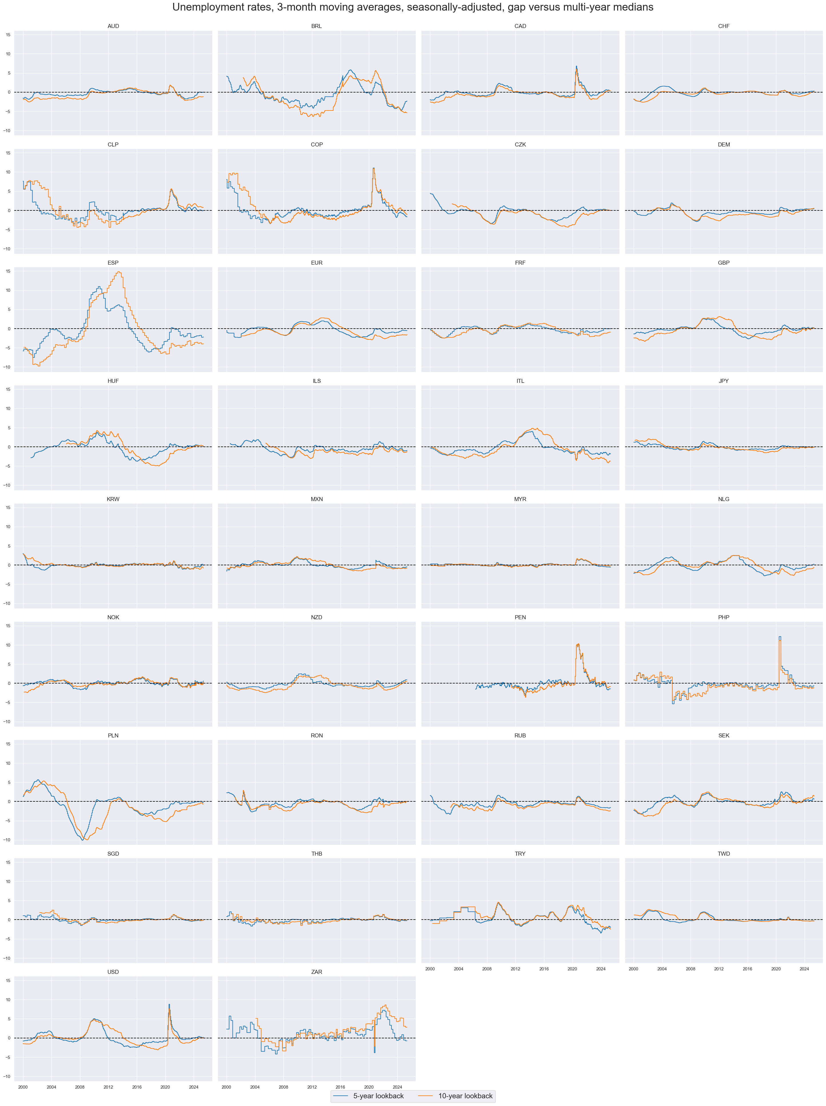
Unemployment rate gaps versus 5-10 year medians #
Empirically, the use of medians rather than means for long-term moving averages does not greatly change the unemployment gap time series. However, it reduces the impact of outlier periods on the multi-year average.
xcatx = ["UNEMPLRATE_SA_3MMAv5YMM", "UNEMPLRATE_SA_3MMAv10YMM"]
cidx = cids_exp

msp.view_ranges(
    dfd,
    xcats=xcatx,
    cids=cidx,
    sort_cids_by="mean",
    start=start_date,
    title="Means and standard deviations of unemployment rate gaps, since 2000",
    xcat_labels=[
        "3-month moving average vs 5-year moving median, (sa)",
        "3-month moving average vs 10-year moving median, (sa)",
    ],
    kind="bar",
    size=(16, 8),
)
xcatx = ["UNEMPLRATE_SA_3MMAv5YMM", "UNEMPLRATE_SA_3MMAv10YMM"]
cidx = cids_exp

msp.view_timelines(
    dfd,
    xcats=xcatx,
    cids=cidx,
    start=start_date,
    title="Unemployment rates, 3-month moving averages, seasonally-adjusted, gap versus multi-year medians",
    xcat_labels=["5-year lookback", "10-year lookback"],
    legend_fontsize=18,
    title_fontsize=27,
    ncol=4,
    same_y=True,
    size=(12, 7),
    aspect=1.7,
    all_xticks=False,
)
Importance #
Research links #
“We investigate both theoretically and empirically how unemployment level and its growth affect future stock returns. We find that both a higher unemployment rate and higher growth of unemployment positively predict future stock market returns.We investigate both theoretically and empirically how unemployment level and its growth affect future stock returns. We find that both a higher unemployment rate and higher growth of unemployment positively predict future stock market returns.” Li & Suominen
“We propose a…model that can account for a long-run joint relationship between inflation, unemployment, and equity prices. The model predicts…a positive relationship between inflation and unemployment….a negative relationship between unemployment and equity prices; and…a negative relationship between inflation and equity prices. Empirical evidence for this trivariate relationship in the post-WWII US data has been documented in previous studies.” Jung & Pyun
Empirical clues #
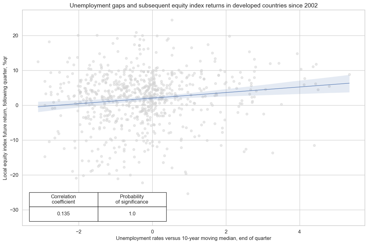
Relatively high unemployment should benefit broad equity return performance, as it supports accommodative monetary policy conditions and reduces wage pressure. Indeed, there has been significant positive correlation between unemployment rates and subsequent equity returns across developed markets.
cids_eq = dfd[dfd["xcat"] == "EQXR_NSA"]["cid"].unique()
cidx = list(set(cids_dmca).intersection(set(cids_eq)))

cr = msp.CategoryRelations(
    dfd,
    xcats=["UNEMPLRATE_SA_3MMAv10YMM", "EQXR_NSA"],
    cids=cidx,
    freq="Q",
    lag=1,
    xcat_aggs=["last", "sum"],
    start="2002-01-01",
)
cr.reg_scatter(
    title="Unemployment gaps and subsequent equity index returns in developed countries since 2002",
    labels=False,
    coef_box="lower left",
    ylab="Local equity index future return, following quarter, %qr",
    xlab="Unemployment rates versus 10-year moving median, end of quarter",
)
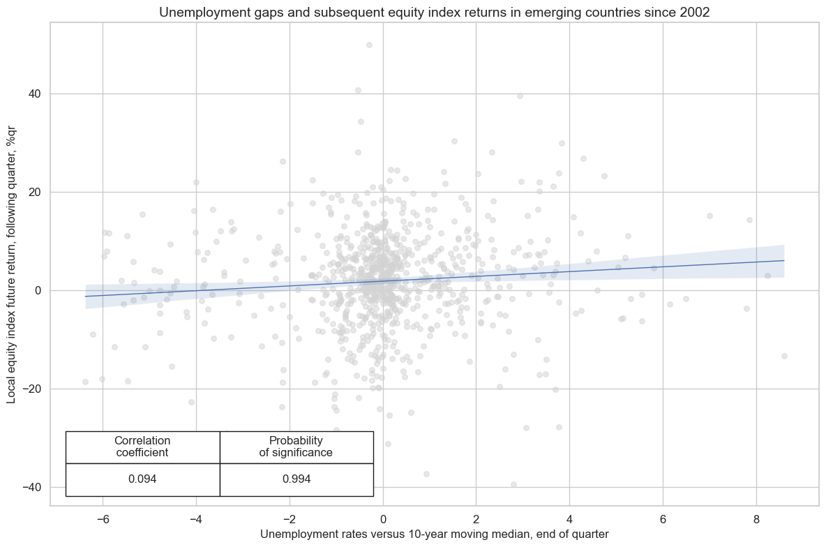
Evidence of a positive correlation also prevails amongst emerging markets, but it is weaker.
cids_eq = dfd[dfd["xcat"] == "EQXR_NSA"]["cid"].unique()
cids_sel = list(set(cids_em) & set(cids_eq) - set(["CNY", "INR"]))
cr = msp.CategoryRelations(
    dfd,
    xcats=["UNEMPLRATE_SA_3MMAv10YMM", "EQXR_NSA"],
    cids=cids_sel,
    freq="Q",
    lag=1,
    xcat_aggs=["last", "sum"],
    start="2002-01-01",
)

cr.reg_scatter(
    title="Unemployment gaps and subsequent equity index returns in emerging countries since 2002",
    labels=False,
    coef_box="lower left",
    ylab="Local equity index future return, following quarter, %qr",
    xlab="Unemployment rates versus 10-year moving median, end of quarter",
)
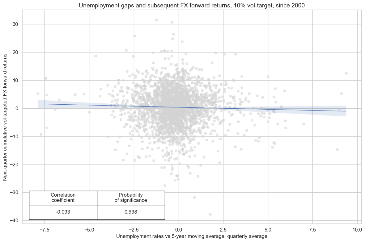
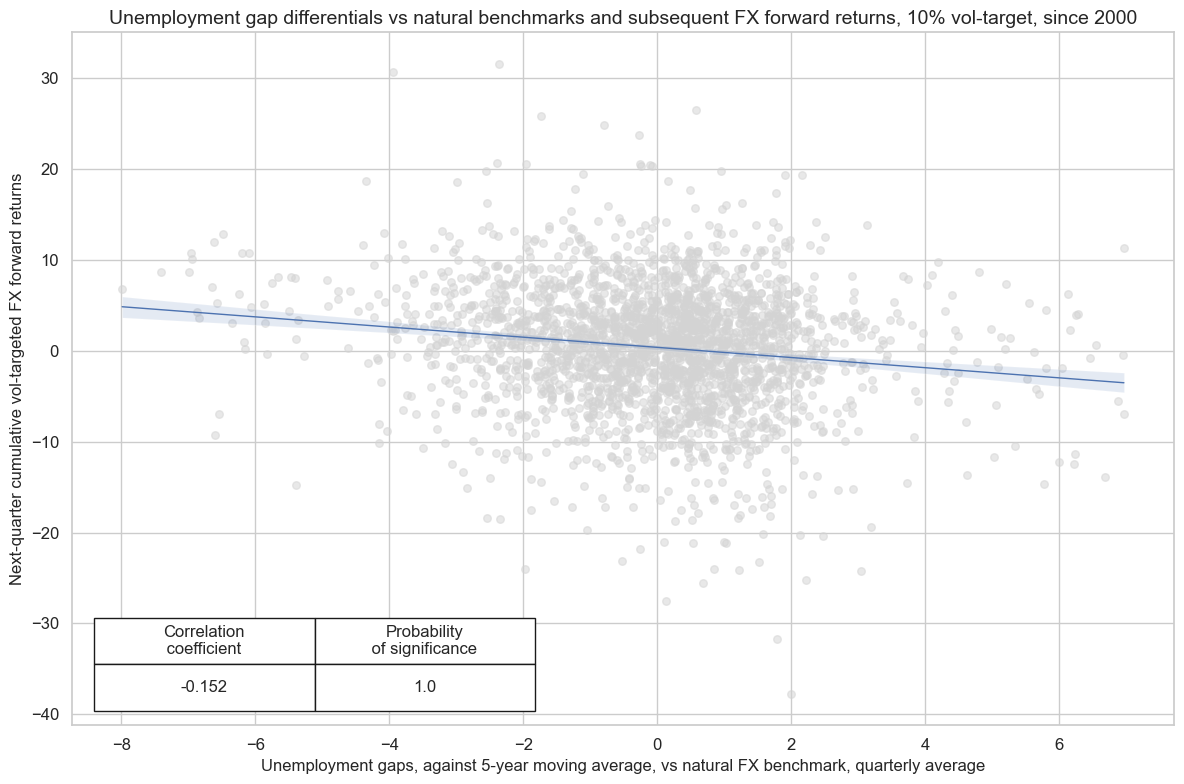
Greater unemployment gaps lead to periods of reduced public spending, leading to a slowdown in economic activity and greater economic instability. This creates risk from the perspective of an investor and can consequently reduce demand for the currency, resulting in smaller FX forward rates against the dollar. This is more easily seen in JPMaQS by regressing FX forward returns (or vol-targeted returns) against unemployment gap differentials vs the natural FX benchmark for the currency area.
See the notes for ‘FX forward return in % of notional’ here for more information on the benchmarks used for each cross-section.
# create blacklist for targeted/untradeable currencies

dfb = dfd[dfd["xcat"].isin(["FXTARGETED_NSA", "FXUNTRADABLE_NSA"])].loc[
    :, ["cid", "xcat", "real_date", "value"]
]
dfba = (
    dfb.groupby(["cid", "real_date"])
    .aggregate(value=pd.NamedAgg(column="value", aggfunc="max"))
    .reset_index()
)
dfba["xcat"] = "FXBLACK"
fxblack = msp.make_blacklist(dfba, "FXBLACK")
# Feature engineer the unemployment gap differentials vs natural benchmarks

cidx = cids_exp

cids_eur = ["CHF", "CZK", "HUF", "NOK", "PLN", "RON", "SEK"]  # EUR benchmark cids
cids_eud = ["GBP", "TRY", "RUB"]  # mean(EUR,USD) benchmark cids
cids_usd = list(set(cidx) - set(cids_eur) - set(cids_eud))  # USD benchmark cids

xcatx = ["UNEMPLRATE_SA_3MMAv5YMM", "UNEMPLRATE_SA_3MMAv10YMM"]
xcatx += ["UNEMPLRATE_SA_3MMAv5YMA", "UNEMPLRATE_SA_3MMAv10YMA"]

for xc in xcatx:
    calc_eur = [f"{xc}vBM = {xc} - iEUR_{xc}"]
    calc_usd = [f"{xc}vBM = {xc} - iUSD_{xc}"]
    calc_eud = [f"{xc}vBM = {xc} - 0.5 * ( iEUR_{xc} + iUSD_{xc} )"]

    dfa_eur = msp.panel_calculator(dfd, calcs=calc_eur, cids=cids_eur)
    dfa_usd = msp.panel_calculator(dfd, calcs=calc_usd, cids=cids_usd)
    dfa_eud = msp.panel_calculator(dfd, calcs=calc_eud, cids=cids_eud)

    dfa = pd.concat([dfa_eur, dfa_usd, dfa_eud])
    dfd = msm.update_df(dfd, dfa)
# Unemployment gap, no benchmark

xcatx = ["UNEMPLRATE_SA_3MMAv5YMA", "FXXR_VT10"]
cidx = list(set(cids_exp) - set(["USD"]))

cr = msp.CategoryRelations(
    df=dfd,
    xcats=xcatx,
    cids=cidx,
    start="2000-01-01",
    blacklist=fxblack,
    freq="Q",
    lag=1,
    xcat_aggs=["mean", "sum"],
)
cr.reg_scatter(
    coef_box="lower left",
    prob_est="map",
    title="Unemployment gaps and subsequent FX forward returns, 10% vol-target, since 2000",
    xlab="Unemployment rates vs 5-year moving average, quarterly average",
    ylab="Next-quarter cumulative vol-targeted FX forward returns",
)

# Unemployment gap vs natural benchmark

xcatx = ["UNEMPLRATE_SA_3MMAv5YMAvBM", "FXXR_VT10"]
cidx = list(set(cids_exp) - set(["USD"]))

cr = msp.CategoryRelations(
    df=dfd,
    xcats=xcatx,
    cids=cidx,
    start="2000-01-01",
    blacklist=fxblack,
    freq="Q",
    lag=1,
    xcat_aggs=["mean", "sum"],
)
cr.reg_scatter(
    coef_box="lower left",
    prob_est="map",
    title="Unemployment gap differentials vs natural benchmarks and subsequent FX forward returns, 10% vol-target, since 2000",
    xlab="Unemployment gaps, against 5-year moving average, vs natural FX benchmark, quarterly average",
    ylab="Next-quarter cumulative vol-targeted FX forward returns",
)
FXXR_VT10 misses: ['DEM', 'ESP', 'FRF', 'ITL', 'NLG'].
FXXR_VT10 misses: ['DEM', 'ESP', 'FRF', 'ITL', 'NLG'].
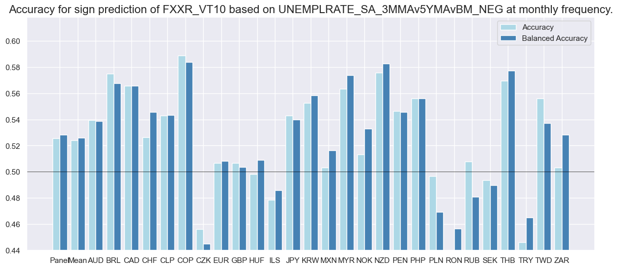
For a number of cross-sections, there is evidence in favour of using the inverse sign of the unemployment gap differentials as a simple feature for predicting the direction of subsequent cumulative FX forward returns (with vol-targeting).
xcatx = ["UNEMPLRATE_SA_3MMAv5YMAvBM", "FXXR_VT10"]
cidx = list(set(cids_exp) - set(["USD"]))

sr = mss.SignalReturnRelations(
    df=dfd,
    rets=xcatx[1],
    sigs=[xcatx[0], "UNEMPLRATE_SA_3MMAv5YMA"],
    cids=cidx,
    sig_neg=[True, True],
    start="2000-01-01",
    blacklist=fxblack,
    agg_sigs="mean",
    freqs="M",
)
sr.accuracy_bars()
Appendices #
Appendix 1: Currency symbols #
The word ‘cross-section’ refers to currencies, currency areas or economic areas. In alphabetical order, these are AUD (Australian dollar), BRL (Brazilian real), CAD (Canadian dollar), CHF (Swiss franc), CLP (Chilean peso), CNY (Chinese yuan renminbi), COP (Colombian peso), CZK (Czech Republic koruna), DEM (German mark), ESP (Spanish peseta), EUR (Euro), FRF (French franc), GBP (British pound), HKD (Hong Kong dollar), HUF (Hungarian forint), IDR (Indonesian rupiah), ITL (Italian lira), JPY (Japanese yen), KRW (Korean won), MXN (Mexican peso), MYR (Malaysian ringgit), NLG (Dutch guilder), NOK (Norwegian krone), NZD (New Zealand dollar), PEN (Peruvian sol), PHP (Phillipine peso), PLN (Polish zloty), RON (Romanian leu), RUB (Russian ruble), SEK (Swedish krona), SGD (Singaporean dollar), THB (Thai baht), TRY (Turkish lira), TWD (Taiwanese dollar), USD (U.S. dollar), ZAR (South African rand).