Consumer price inflation trends #
This category group contains real-time measures of various latest headline and core consumer price trends and changes thereof. The measures are based on actual and estimated vintages of common local standards of consumer price measures. In particular, data vintages use sequentially updating algorithmic adjustments for seasonal factors, jumps, and temporary spikes to allow calculations of trends in line with standard analyses of economists.
Annual headline consumer price inflation #
Ticker : CPIH_SA_P1M1ML12
Label : Standard annual headline consumer price inflation.
Definition : Most widely watched consumer price measure of the currency area, % change of latest release over a year ago.
Notes :
-
Typically, this inflation rate is based on the main CPI index of a country. In some countries, other indices were used in the past, such as the UK (retail price index) and India (a wholesale price index).
-
The headline consumer price index is not necessarily the one preferred by the central bank, who may focus more on core or net inflation measures. However, it typically does have a significant weight in the public discussion on inflation.
-
The underlying data series are monthly, except Australia and New Zealand, which only produce quarterly official CPIs. A monthly CPI inflation rate for Australia is estimated based on a monthly ‘TD-MI Inflation Gauge’. For New Zealand, only the latest quarterly official CPI data are used.
Seasonally and jump-adjusted headline consumer price trends #
Ticker : CPIH_SJA_P1M1ML1 / _P3M3ML3AR / _P6M6ML6AR
Label : Adjusted headline consumer price trend: % 1m/1m / % 3m/3m ar / % 6m/6m ar.
Definition : Headline consumer price index, seasonally- and jump-adjusted: % of latest month over previous month / % of latest 3 months over previous 3 months at annualized rate / % of latest 6 months over previous 6 months at an annualized rate.
Notes :
-
Seasonal adjustment factors are sequentially re-estimated as new data are released. This means that a new data vintage is created at every estimation. For more detail, see Appendix 3 .
-
Jump adjustment means that two types of outliers are adjusted for. Firstly, large “spikes” (i.e., two subsequent large moves of the seasonal index in opposite directions) are averaged. The causes for such spikes are often holiday shifts between two months, while the causes for jumps are mostly indirect taxes, administered prices, or FX turbulences. Secondly, large one-off jumps in the index are replaced by the local trend. The criteria for adjustment are statistically based on pattern recognition. For more detail, see Appendix 3 .
-
In most markets, shorter-horizon price trends are watched mainly by market economists and not the broader public.
-
For Australia and New Zealand, see notes for ‘annual headline consumer price inflation’.
Change in headline consumer price inflation #
Ticker : CPIH_SA_P1M1ML12_D1M1ML3
Label : Change in annual headline consumer price inflation over the past three months.
Definition : Change in the most widely watched consumer price measure of the currency area, % change of latest release over a year ago, difference of latest released month compared to three months ago.
Notes :
-
Note that this category represents information states of changes (according to latest vintage) and not changes of information changes, which represent updates of vintages and can be calculated directly based on quantamental indicators.
-
See notes for ‘Annual headline consumer price inflation’.
Annual core consumer price inflation #
Ticker : CPIC_SA_P1M1ML12
Label : Annual core consumer price inflation.
Definition : Core consumer price index preferred by the central bank or market, % change of latest release over a year ago.
Notes :
-
Unlike headline consumer prices, this index is chosen based on the local central bank or market convention rather than popular following.
-
The basic idea behind core price indices is to exclude volatile or erratic prices that cloud the detection of a trend. Often, this means excluding specific food and energy products from the basket.
-
The basis for the adjustment is usually a consumer price index. An exception is the U.S., where the central bank has preferred focusing on a price index of personal consumer expenditures.
-
For Australia and New Zealand, see notes for ‘Annual headline consumer price inflation’.
-
For information on the excluded volatile components for each currency area, see Appendix 1 .
Seasonally and jump-adjusted core consumer price trends #
Ticker : CPIC_SJA_P1M1ML1 / _P3M3ML3AR / _P6M6ML6AR
Label : Adjusted latest core consumer price trend: % 1m/1m / % 3m/3m ar / % 6m/6m ar.
Definition : Core consumer price index, seasonally and jump-adjusted: % of latest month over previous month / % of latest 3 months over previous 3 months at an annualized rate / % of latest 6 months over previous 6 months at an annualized rate.
Notes :
-
Seasonal adjustment factors are sequentially re-estimated as new data are released. This means that a new data vintage is created at every estimation.
-
Jump adjustment means that two types of outliers are adjusted for. Firstly, large “spikes” (i.e. two subsequent large moves of the seasonal index in opposite directions) are averaged. The causes for such spikes are often holiday shifts between two months, while the causes for jumps are mostly indirect taxes, administered prices, or FX turbulences. Secondly, the local trend replaces large one-off jumps in the index. The criteria for adjustment are statistically based on pattern recognition.
-
The basis for the adjustment is usually a consumer price index. An exception is the U.S., where the central bank has preferred focusing on a price index of personal consumer expenditures.
-
For Australia and New Zealand, see notes for ‘Annual headline consumer price inflation’.
-
For information on the excluded volatile components for each currency area, see Appendix 1 .
Change in annual core consumer price inflation #
Ticker : CPIC_SA_P1M1ML12_D1M1ML3
Label : Change in annual core consumer price inflation over the past 3 months.
Definition : Change in core consumer price measure preferred by the central bank or market, % change of latest release over a year ago, difference of latest released month compared to three months ago.
Notes :
-
Note that this category represents information states of changes (according to latest vintage) and not changes of information changes, which represent updates of vintages and can be calculated directly based on quantamental indicators.
-
See notes for ‘Annual core consumer price inflation’.
-
The basis for the adjustment is usually a consumer price index. An exception is the U.S., where the central bank has preferred focusing on a price index of personal consumer expenditures.
Headline CPI inflation, using early estimates #
Ticker : CPIHE_SA_P1M1ML12 / CPIHE_SJA_P3M3ML3AR / CPIHE_SJA_P6M6ML6AR / CPIHE_SA_P1M1ML12_D1M1ML3
Label : CPI, using early estimates: % oya / % 3m/3m saar (jump-adjusted) / % 6m/6m saar (jump-adjusted) / change of %oya over 3 months
Definition : Consumer price inflation, using early estimates: % oya / % 3m/3m saar (jump-adjusted) / % 6m/6m saar (jump-adjusted) / change of %oya over 3 months
Notes :
-
These series measure annual headline consumer price inflation similar to standard headline and core categories, but use timely related price indicators for estimating the latest month early. Specifically, the early information is used prior to the release of the official CPI in accordance with convention among market economists. Early indicators of this type have been identified for the following countries: Japan, Turkey, Singapore, Philippines, Mexico, South Africa, Great Britain, Mexico and Russia.
-
There are two types of early estimates. The first is applied to early indicators that are very close to the official CPI. In this case, predictions of the official CPI are made by setting its latest monthly change equal to the early price indicator’s monthly change. The second type of estimate uses a prominent component of the CPI whose price is released earlier. In this case, the latest monthly CPI change is predicted using a regression based on the historic relation between the early indicator’s change in annual growth and the same change for the headline CPI.
-
The following countries have broad CPI proxies that are used directly as predictors: Japan (Tokyo CPI), Mexico (bi-weekly CPI), Russia (weekly CPI), Turkey (Istanbul CPI)
-
The following countries use smaller predictor sets and regression: UK (BRC Nielsen), Singapore (car ownership costs), the Philippines (rice price), and South Africa (white maize price).
-
For further information on the indicator calculations, see Appendix 2 .
Core CPI changes, using early estimates #
Ticker : CPICE_SA_P1M1ML12 / CPICE_SJA_P3M3ML3AR / CPICE_SJA_P6M6ML6AR / CPICE_SA_P1M1ML12_D1M1ML3
Label : Core CPI, using early estimates: % oya / % 3m/3m saar (jump-adjusted) / % 6m/6m saar (jump-adjusted) / change of %oya over 3 months
Definition : Core consumer price inflation, using early estimates: % oya / % 3m/3m saar (jump-adjusted) / % 6m/6m saar (jump-adjusted) / change of %oya over 3 months
Notes :
-
Note that this category represents information states of changes (according to latest vintage) and not changes of information changes, which represent updates of vintages and can be calculated directly based on quantamental indicators.
-
These series measure annual headline consumer price inflation similar to standard headline and core categories, but use timely related price indicators for estimating the latest month early. Specifically, the early information is used prior to the release of the official CPI in accordance with convention among market economists. Early indicators have been identified for the U.S. (core CPI as predictor for core PCE) and Japan (Tokyo core CPI).
-
Predictions of the target core CPIs are made by setting the latest monthly change equal to the early price index’s monthly change.
-
For further information on the indicator calculations, see Appendix 2 .
Imports #
Only the standard Python data science packages and the specialized
macrosynergy
package are needed.
import os
import pandas as pd
import matplotlib.pyplot as plt
import numpy as np

import macrosynergy.management as msm
import macrosynergy.panel as msp
import macrosynergy.signal as mss
import macrosynergy.pnl as msn

from macrosynergy.download import JPMaQSDownload

import warnings
warnings.simplefilter("ignore")
The
JPMaQS
indicators we consider are downloaded using the J.P. Morgan Dataquery API interface within the
macrosynergy
package. This is done by specifying
ticker strings
, formed by appending an indicator category code
<category>
to a currency area code
<cross_section>
. These constitute the main part of a full quantamental indicator ticker, taking the form
DB(JPMAQS,<cross_section>_<category>,<info>)
, where
<info>
denotes the time series of information for the given cross-section and category. The following types of information are available:
-
valuegiving the latest available values for the indicator -
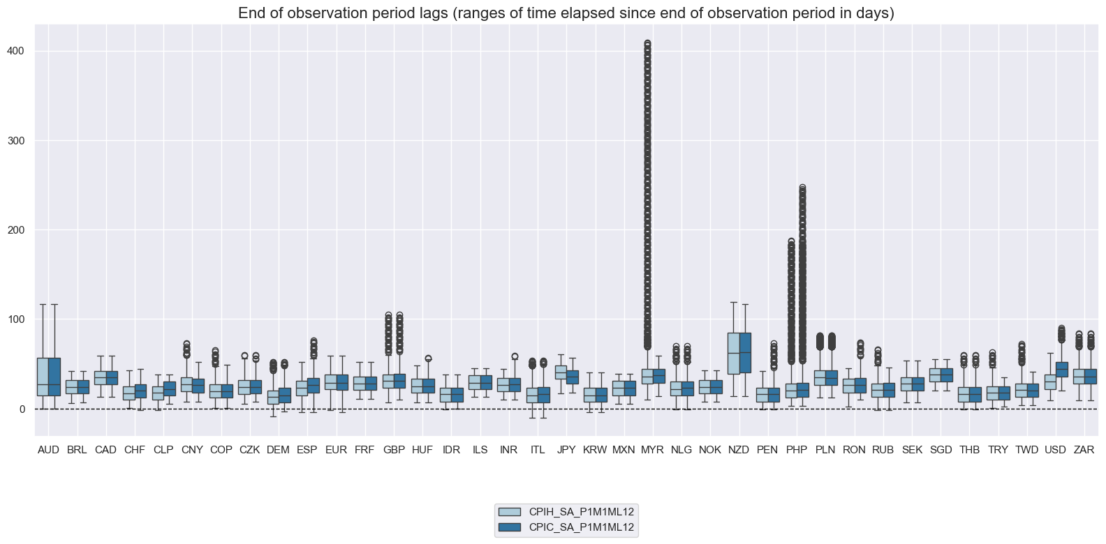
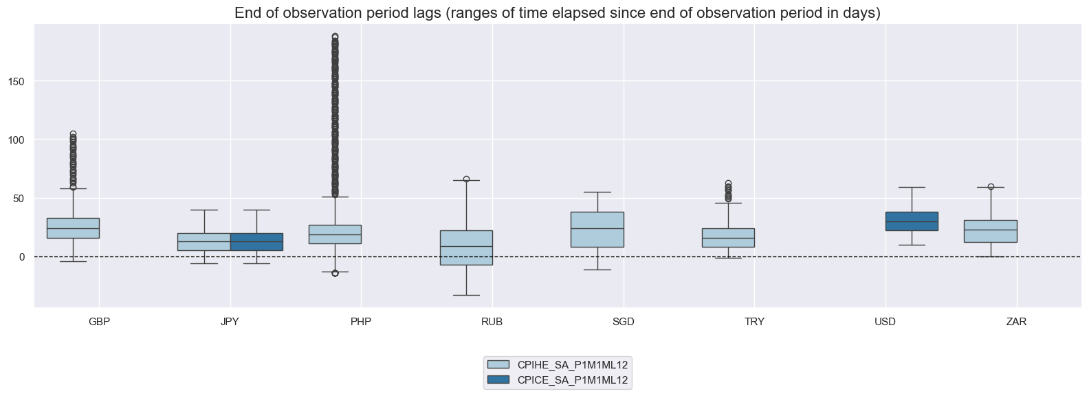
eop_lagreferring to days elapsed since the end of the observation period -
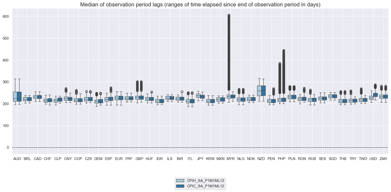
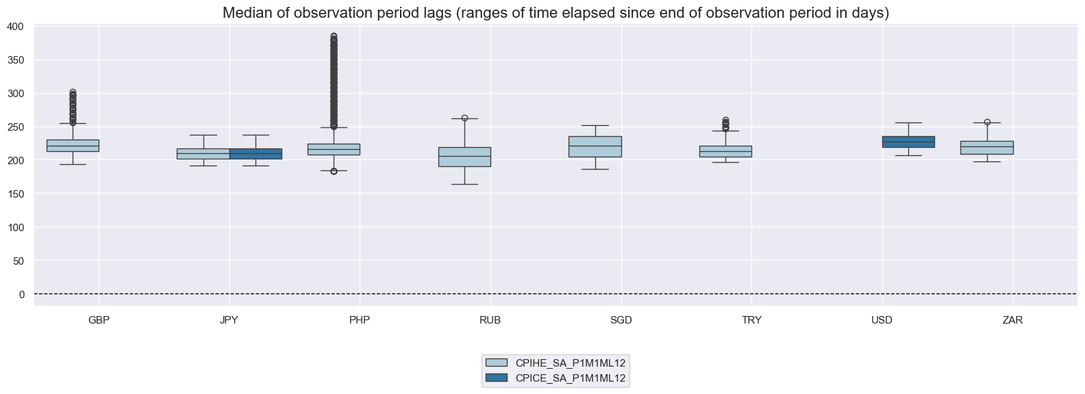
mop_lagreferring to the number of days elapsed since the mean observation period -
gradedenoting a grade of the observation, giving a metric of real time information quality.
After instantiating the
JPMaQSDownload
class within the
macrosynergy.download
module, one can use the
download(tickers,start_date,metrics)
method to easily download the necessary data, where
tickers
is an array of ticker strings,
start_date
is the first collection date to be considered and
metrics
is an array comprising the times series information to be downloaded.
# Cross-sections of interest

cids_dmca = [
    "AUD",
    "CAD",
    "CHF",
    "EUR",
    "GBP",
    "JPY",
    "NOK",
    "NZD",
    "SEK",
    "USD",
]  # DM currency areas
cids_dmec = ["DEM", "ESP", "FRF", "ITL", "NLG"]  # DM euro area countries

cids_dm = cids_dmca + cids_dmec

cids_em = ["BRL", "COP", "CLP", "MXN", "PEN",  # Latam countries
"CZK", "HUF", "ILS", "PLN", "RON", "RUB", "TRY", "ZAR",  # EMEA countries
"CNY", "IDR", "INR", "KRW", "MYR", "PHP", "SGD", "THB", "TWD"] # Asia countries

cids_early = ["GBP", "JPY", "USD", "RUB", "TRY", "ZAR", "PHP", "SGD"]

cids = sorted(cids_dm + cids_em)
# Quantamental categories of interest

main = [
    "CPIC_SA_P1M1ML12",
    "CPIC_SJA_P1M1ML1",
    "CPIC_SJA_P3M3ML3AR",
    "CPIC_SJA_P6M6ML6AR",
    "CPIC_SA_P1M1ML12_D1M1ML3",
    "CPIH_SA_P1M1ML12",
    "CPIH_SJA_P1M1ML1",
    "CPIH_SJA_P3M3ML3AR",
    "CPIH_SJA_P6M6ML6AR",
    "CPIH_SA_P1M1ML12_D1M1ML3",
]
early = [
    "CPIHE_SA_P1M1ML12",
    "CPIHE_SJA_P3M3ML3AR",
    "CPIHE_SJA_P6M6ML6AR",
    "CPIHE_SA_P1M1ML12_D1M1ML3",
    "CPICE_SA_P1M1ML12",
    "CPICE_SJA_P3M3ML3AR",
    "CPICE_SJA_P6M6ML6AR",
    "CPICE_SA_P1M1ML12_D1M1ML3",
]

misc = ["INFTEFF_NSA", "INFTARGET_NSA"] # Inflation targets

mark = ["EQXR_NSA",
        "EQXR_VT10",
        "DU02YXR_VT10",
        "DU02YXR_NSA",
        "DU05YXR_VT10",
        "FXXR_VT10",
        "GB01YR_NSA",
        "GB02YR_NSA",
        "GB03YR_NSA",
        "GB05YR_NSA",
        "GB01YYLD_NSA"]  # market links

xcats = main + early + mark + misc
# Download series from J.P. Morgan DataQuery by tickers

start_date = "1990-01-01"
tickers = [cid + "_" + xcat for cid in cids for xcat in xcats]
print(f"Maximum number of tickers is {len(tickers)}")

# Retrieve credentials

client_id: str = os.getenv("DQ_CLIENT_ID")
client_secret: str = os.getenv("DQ_CLIENT_SECRET")

with JPMaQSDownload(client_id=client_id, client_secret=client_secret) as dq:
    df = dq.download(
        tickers=tickers,
        start_date=start_date,
        suppress_warning=True,
        metrics=["all"],
        show_progress=True,
    )
Maximum number of tickers is 1147
Downloading data from JPMaQS.
Timestamp UTC:  2025-03-26 09:19:09
Connection successful!
Requesting data: 100%|███████████████████████████████████████████████████████████████| 230/230 [00:52<00:00,  4.39it/s]
Downloading data: 100%|██████████████████████████████████████████████████████████████| 230/230 [01:17<00:00,  2.95it/s]
Some expressions are missing from the downloaded data. Check logger output for complete list.
1840 out of 4588 expressions are missing. To download the catalogue of all available expressions and filter the unavailable expressions, set `get_catalogue=True` in the call to `JPMaQSDownload.download()`.
Some dates are missing from the downloaded data.
2 out of 9195 dates are missing.
Availability #
cids_exp = sorted(cids)  # cids expected in category panels
msm.missing_in_df(df, xcats=main, cids=cids_exp)
Show code cell output
No missing XCATs across DataFrame.
Missing cids for CPIC_SA_P1M1ML12:          []
Missing cids for CPIC_SA_P1M1ML12_D1M1ML3:  []
Missing cids for CPIC_SJA_P1M1ML1:          []
Missing cids for CPIC_SJA_P3M3ML3AR:        []
Missing cids for CPIC_SJA_P6M6ML6AR:        []
Missing cids for CPIH_SA_P1M1ML12:          []
Missing cids for CPIH_SA_P1M1ML12_D1M1ML3:  []
Missing cids for CPIH_SJA_P1M1ML1:          []
Missing cids for CPIH_SJA_P3M3ML3AR:        []
Missing cids for CPIH_SJA_P6M6ML6AR:        []
cids_early = sorted(list(set(cids_early) - set(cids_dmec)))  # cids expected in category panels
msm.missing_in_df(df, xcats=early, cids=cids_early)
No missing XCATs across DataFrame.
Missing cids for CPICE_SA_P1M1ML12:          ['GBP', 'PHP', 'RUB', 'SGD', 'TRY', 'ZAR']
Missing cids for CPICE_SA_P1M1ML12_D1M1ML3:  ['GBP', 'PHP', 'RUB', 'SGD', 'TRY', 'ZAR']
Missing cids for CPICE_SJA_P3M3ML3AR:        ['GBP', 'PHP', 'RUB', 'SGD', 'TRY', 'ZAR']
Missing cids for CPICE_SJA_P6M6ML6AR:        ['GBP', 'PHP', 'RUB', 'SGD', 'TRY', 'ZAR']
Missing cids for CPIHE_SA_P1M1ML12:          ['USD']
Missing cids for CPIHE_SA_P1M1ML12_D1M1ML3:  ['USD']
Missing cids for CPIHE_SJA_P3M3ML3AR:        ['USD']
Missing cids for CPIHE_SJA_P6M6ML6AR:        ['USD']
Real-time quantamental indicators of consumer price inflation trends for developed markets have been typically available by the late 1990s. Data are available, for some emerging markets, from 1990 onwards.
For the explanation of currency symbols related to currency areas or countries for which categories are available, please view Appendix 3 .
msm.check_availability(
    df,
    xcats=main,
    cids=cids_exp,
    missing_recent=False,
)

Only a small subset of countries have CPI inflation indicators based on early indicators. Most of them go back to the 1990s.
msm.check_availability(
    df,
    xcats=early,
    cids=cids_early,
    missing_recent=False,
)

Vintage grading is mixed. USD is the only cross-section that posted the highest average grades back to the 1990s.
xcatx = main
cidx = cids_exp

plot = msp.heatmap_grades(
    df,
    xcats=xcatx,
    cids=cidx,
    size=(18, 6),
    title=f"Average vintage grades from {start_date} onwards",
)

xcatx = early
cidx = cids_early

plot = msp.heatmap_grades(
    df,
    xcats=xcatx,
    cids=cidx,
    size=(18, 4),
    title=f"Average vintage grades from {start_date} onwards",
)

The variable
eop_lag
(or
mop_lag
) represents the count of days that have passed since the last (median) of the observation period. Graphing the ranges and timelines of this indicator illustrates the frequency of updates and reveals the fluctuations it has undergone over time.
xcatx = ["CPIH_SA_P1M1ML12", "CPIC_SA_P1M1ML12"]
cidx = cids_exp

msp.view_ranges(
    df,
    xcats=xcatx,
    cids=cidx,
    val="eop_lag",
    title="End of observation period lags (ranges of time elapsed since end of observation period in days)",
    start=start_date,
    kind="box",
 )
msp.view_ranges(
    df,
    xcats=xcatx,
    cids=cidx,
    val="mop_lag",
    title="Median of observation period lags (ranges of time elapsed since end of observation period in days)",
    start=start_date,
    kind="box",

)
cidx = ["USD", "EUR", "GBP"]

msp.view_timelines(
    df,
    xcats="CPIC_SA_P1M1ML12",
    cids=cidx,
    val="eop_lag"
)

xcatx = ["CPIHE_SA_P1M1ML12", "CPICE_SA_P1M1ML12"]
cidx = cids_early

msp.view_ranges(
    df,
    xcats=xcatx,
    cids=cidx,
    val="eop_lag",
    title="End of observation period lags (ranges of time elapsed since end of observation period in days)",
    start=start_date,
    kind="box",
    size=(16, 6),
)
msp.view_ranges(
    df,
    xcats=xcatx,
    cids=cidx,
    val="mop_lag",
    title="Median of observation period lags (ranges of time elapsed since end of observation period in days)",
    start=start_date,
    kind="box",
    size=(16, 6),
)
History #
Annual headline/core consumer price inflation #
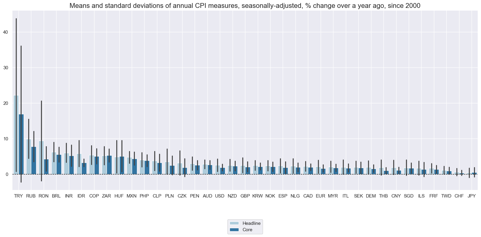
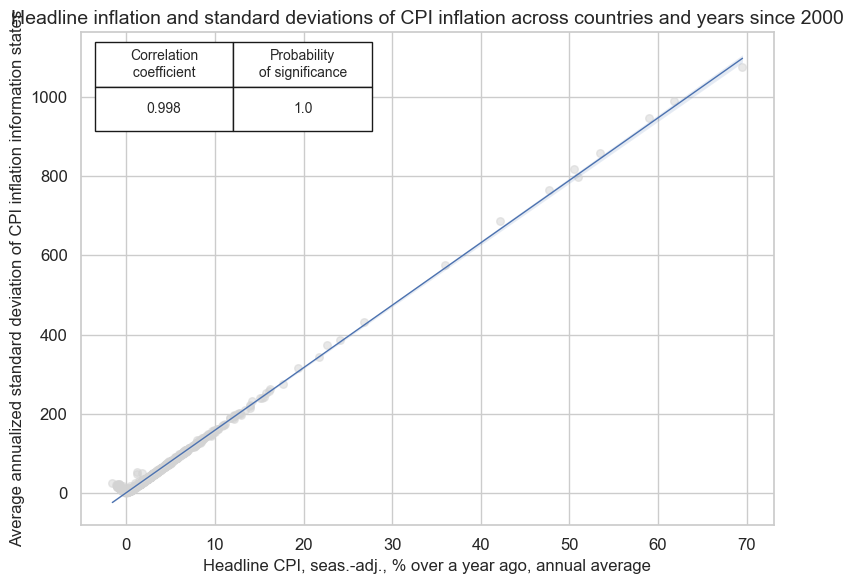
Since 2000, headline inflation averages and variances have been materially different across countries. Importantly, there has been a clear linear relation between average inflation and its standard deviation, across currency areas and years. This suggests high inflation comes with high uncertainty.
xcatx = ["CPIH_SA_P1M1ML12", "CPIC_SA_P1M1ML12"]
cidx = cids_exp

msp.view_ranges(
    df,
    xcats=xcatx,
    cids=cidx,
    sort_cids_by="mean",
    start="2000-01-01",
    kind="bar",
    title="Means and standard deviations of annual CPI measures, seasonally-adjusted, % change over a year ago, since 2000",
    xcat_labels=["Headline", "Core"],
    size=(16, 8),
)
dfa = msp.historic_vol(
    df, xcat="CPIH_SA_P1M1ML12", cids=cids, lback_meth="xma", postfix="_ASD"
)
df = msm.update_df(df, dfa)

cr_infl_vol = msp.CategoryRelations(
    df,
    xcats=["CPIH_SA_P1M1ML12", 'CPIH_SA_P1M1ML12_ASD'],
    cids=cids,
    freq="A",
    lag=0,
    xcat_aggs=["mean", "mean"],
    start="2000-01-01",

)

cr_infl_vol.reg_scatter(
    labels=False,
    coef_box="upper left",
    xlab="Headline CPI, seas.-adj., % over a year ago, annual average",
    ylab="Average annualized standard deviation of CPI inflation information states",
    title="Headline inflation and standard deviations of CPI inflation across countries and years since 2000",
    size=(8, 6),
    prob_est="map",
)
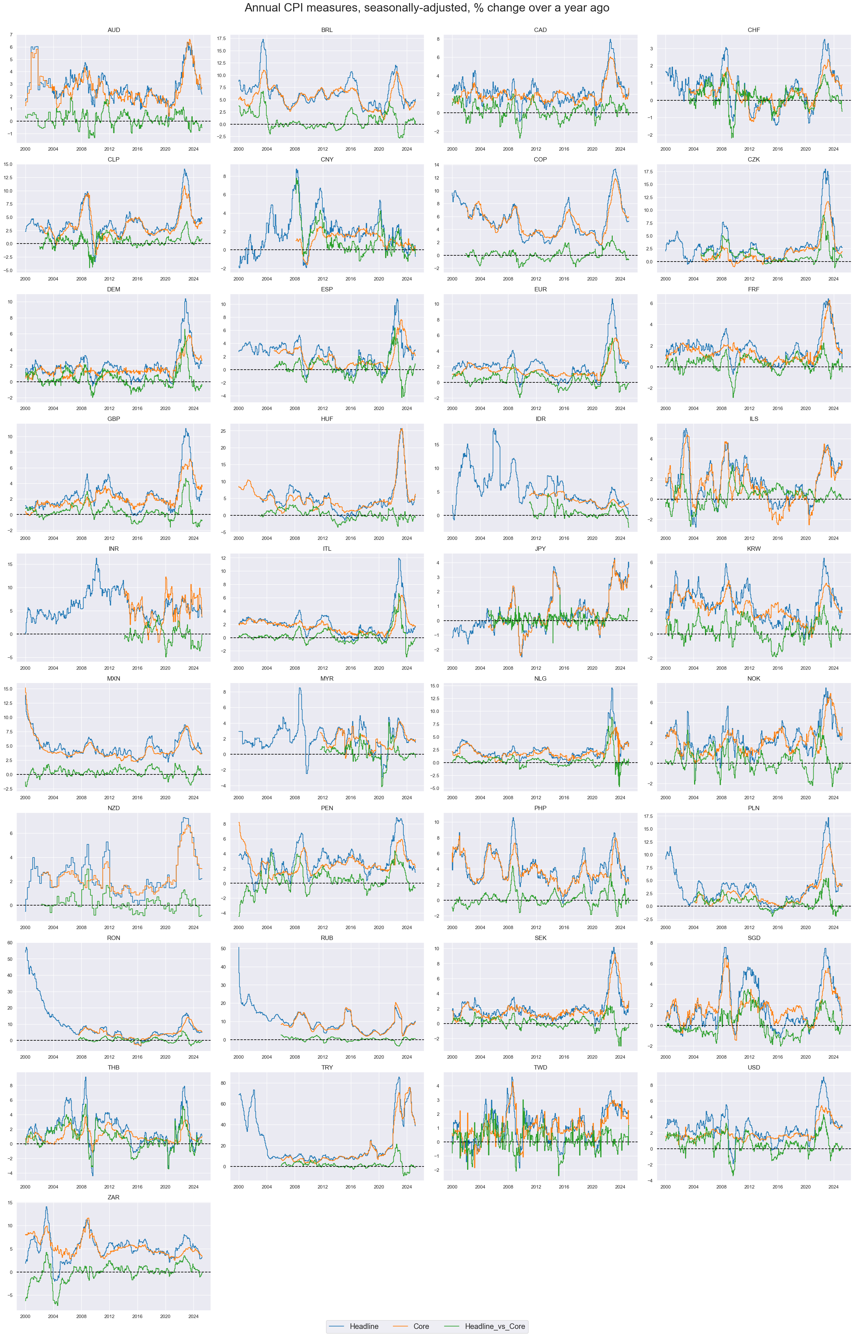
Headline and core inflation can deviate materially, testifying to the power and volatility of food and energy prices.
cidx = cids_exp
calcs = ["Headline_vs_Core = CPIH_SA_P1M1ML12 - CPIC_SA_P1M1ML12"]
xcatx = ["CPIH_SA_P1M1ML12", "CPIC_SA_P1M1ML12", "Headline_vs_Core"]
dfa = msp.panel_calculator(df, calcs, cids=cids)
df = msm.update_df(df, dfa)


msp.view_timelines(
    df,
    xcats=xcatx,
    cids=cidx,
    start="2000-01-01",
    title="Annual CPI measures, seasonally-adjusted, % change over a year ago",
    title_fontsize=27,
    legend_fontsize=17,
    xcat_labels=["Headline", "Core", "Headline_vs_Core"],
    ncol=4,
    same_y=False,
    all_xticks=True,
)
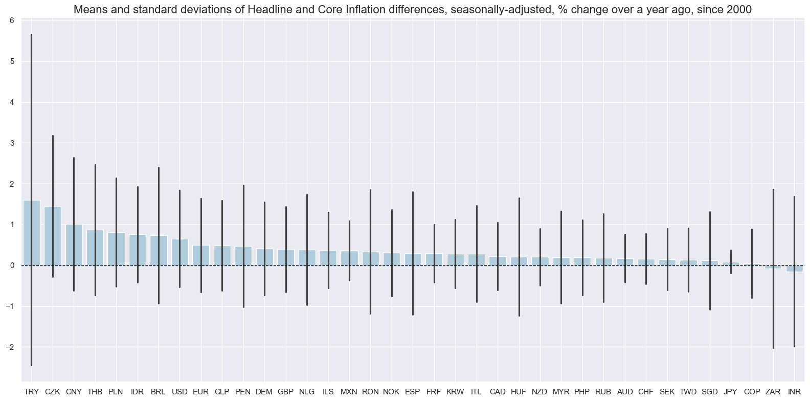
The basic idea behind core price indices is to exclude volatile or erratic prices that cloud the detection of a trend. Core inflation is seen as more stable measure with lower averages and variabilities for most countries. The difference and variability of this difference varies considerably among cross-sections. “The implicit assumption behind the removal of volatile items from core inflation measures is not only that those price changes are volatile but mainly temporary” IMF Working Paper WP15/8
calcs = ["Headline_vs_Core = CPIH_SA_P1M1ML12 - CPIC_SA_P1M1ML12"]
dfa = msp.panel_calculator(df, calcs, cids=cids)
df = msm.update_df(df, dfa)

xcatx = ["Headline_vs_Core"]
cidx = cids_exp

msp.view_ranges(
    df,
    xcats=xcatx,
    cids=cidx,
    sort_cids_by="mean",
    start="2000-01-01",
    kind="bar",
    title="Means and standard deviations of Headline and Core Inflation differences, seasonally-adjusted, % change over a year ago, since 2000",
    size=(16, 8),
)
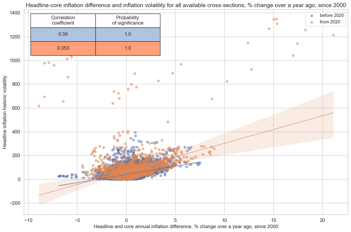
The absolute difference between headline and core inflation rates seems to exhibit a positive correlation with the volatility of headline inflation. This relationship strenghened since the Pandemic:
cr_hvscore_vol = msp.CategoryRelations(
    df,
    xcats=["Headline_vs_Core", 'CPIH_SA_P1M1ML12_ASD'],
    cids=cids,
    freq="M",
    lag=0,
    xcat_aggs=["mean", "mean"],
    start="2000-01-01",

)

cr_hvscore_vol.reg_scatter(
    labels=False,
    coef_box="upper left",
    xlab="Headline and core annual inflation difference, % change over a year ago, since 2000",
    ylab="Headline inflation historic volatility",
    title="Headline-core inflation difference and inflation volatility for all available cross-sections, % change over a year ago, since 2000",
    size=(12, 8),
    prob_est="map",
    separator=2020
    )
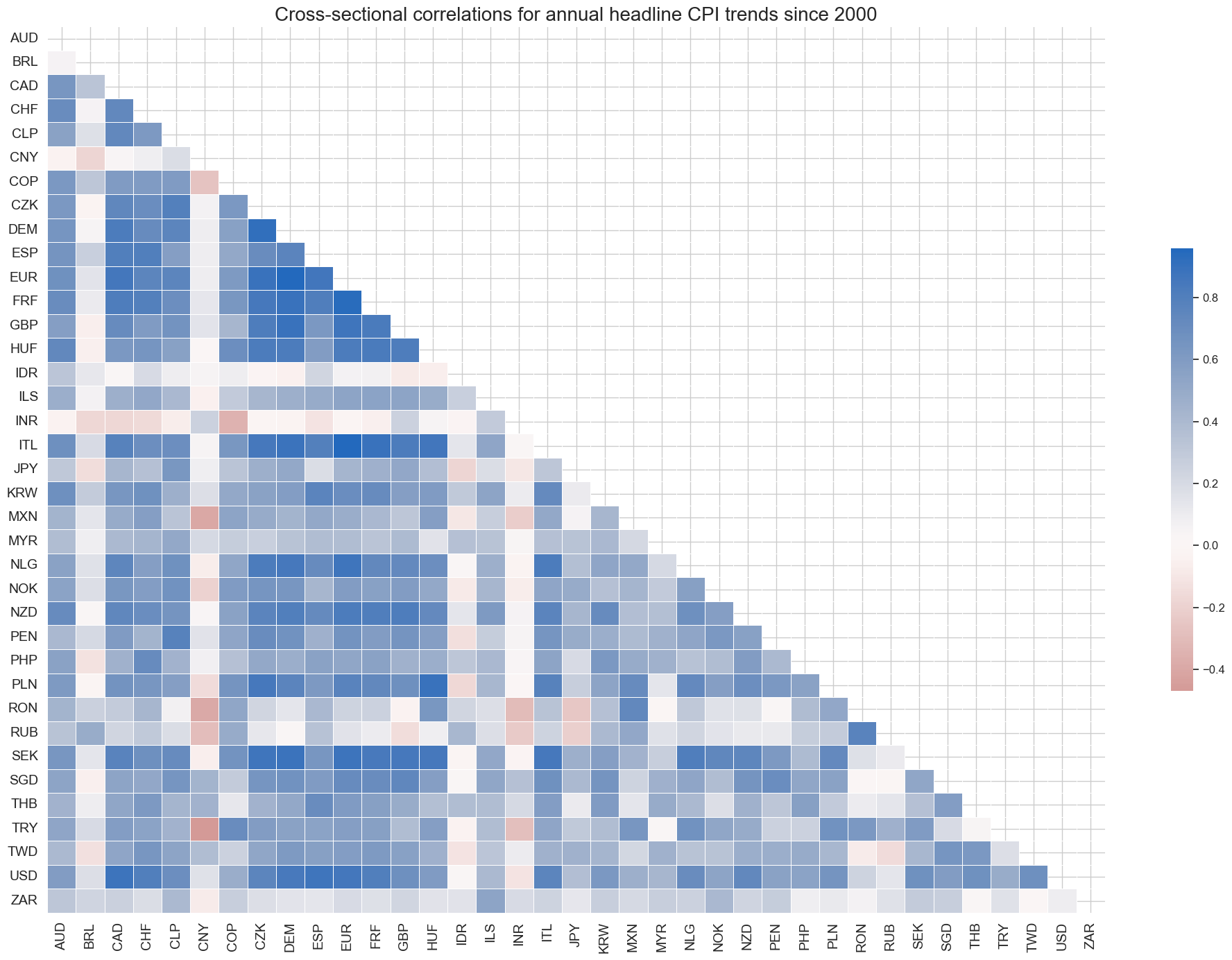
Cross-sectional correlations of headline annual CPI inflation have been predominantly positive since 1990. India and China stand out in displaying the least correlation with other countries. India has a peculiar basket geared towards very low-income earners and used a wholesale price index for the most-watched inflation reports until the 2010s.
xcatx = "CPIH_SA_P1M1ML12"
cidx = cids_exp

msp.correl_matrix(
    df,
    xcats=xcatx,
    cids=cidx,
    title="Cross-sectional correlations for annual headline CPI trends since 2000",
    start="2000-01-01",
    size=(20, 14),
)
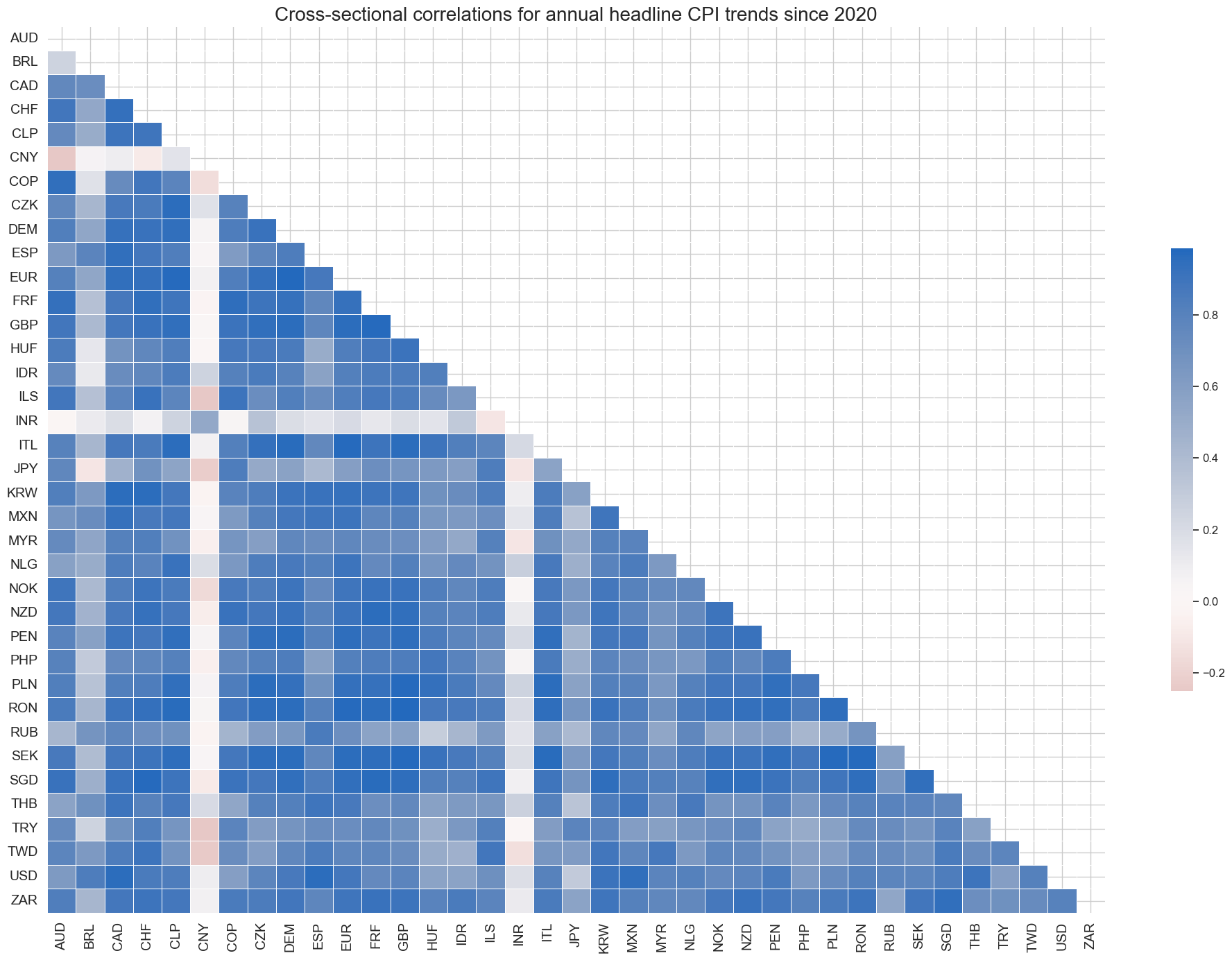
Headline inflation correlation has strengthened since 2020 for majority of countries. India and China remained the least correlated.
xcatx = "CPIH_SA_P1M1ML12"
cidx = cids_exp

msp.correl_matrix(
    df,
    xcats=xcatx,
    cids=cidx,
    title="Cross-sectional correlations for annual headline CPI trends since 2020",
    start="2020-01-01",
    size=(20, 14),
)
Shorter-term headline inflation trends #
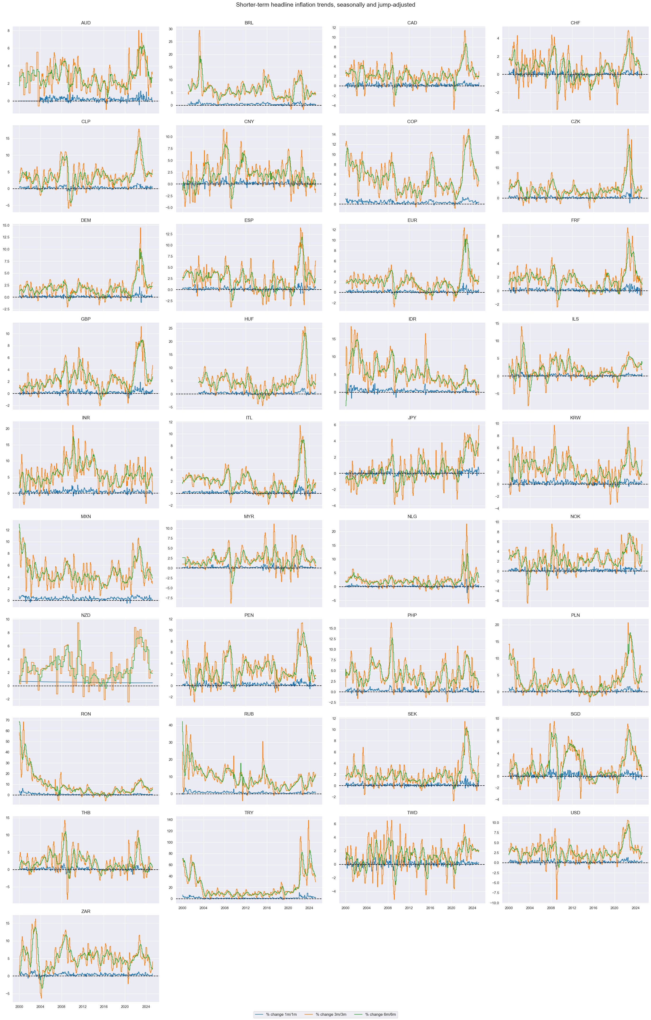
For most countries the 6-month over previous 6-month percentage changes appear to be a far more stable trend indicator than the 3-month over 3-month percentage change series. Moreover, the 6-month over 6-month changes only added a short lag in indicating turning points.
xcatx = ["CPIH_SJA_P1M1ML1","CPIH_SJA_P3M3ML3AR", "CPIH_SJA_P6M6ML6AR"]
cidx = cids_exp

msp.view_timelines(
    df,
    xcats=xcatx,
    cids=cidx,
    start="2000-01-01",
    title="Shorter-term headline inflation trends, seasonally and jump-adjusted",
    xcat_labels=["% change 1m/1m","% change 3m/3m", "% change 6m/6m"],
    ncol=4,
    same_y=False,

)
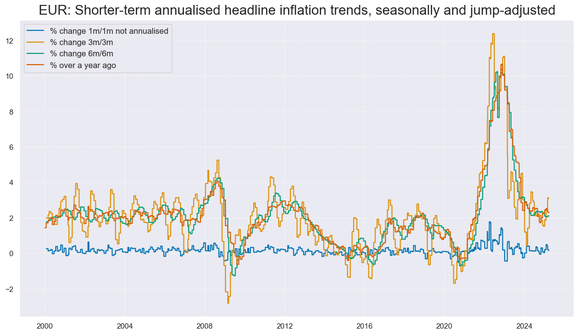
Since these simple CPI trends only depend on official price index releases and revisions are very small, indicator values for most countries tend to change stepwise once or twice a month.
xcatx = ["CPIH_SJA_P1M1ML1","CPIH_SJA_P3M3ML3AR", "CPIH_SJA_P6M6ML6AR", "CPIH_SA_P1M1ML12"]
cidx = "EUR"

msp.view_timelines(
    df,
    xcats=xcatx,
    cids=cidx,
    start="2000-01-01",
    title=f"{cidx}: Shorter-term annualised headline inflation trends, seasonally and jump-adjusted",
    title_fontsize=20,
    xcat_labels=["% change 1m/1m not annualised","% change 3m/3m", "% change 6m/6m", "% over a year ago"],
    ncol=2,
    same_y=False,

)
Change in headline consumer price inflation #
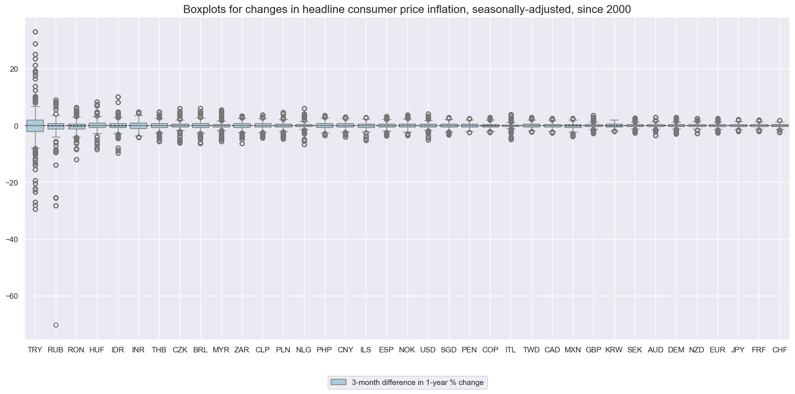
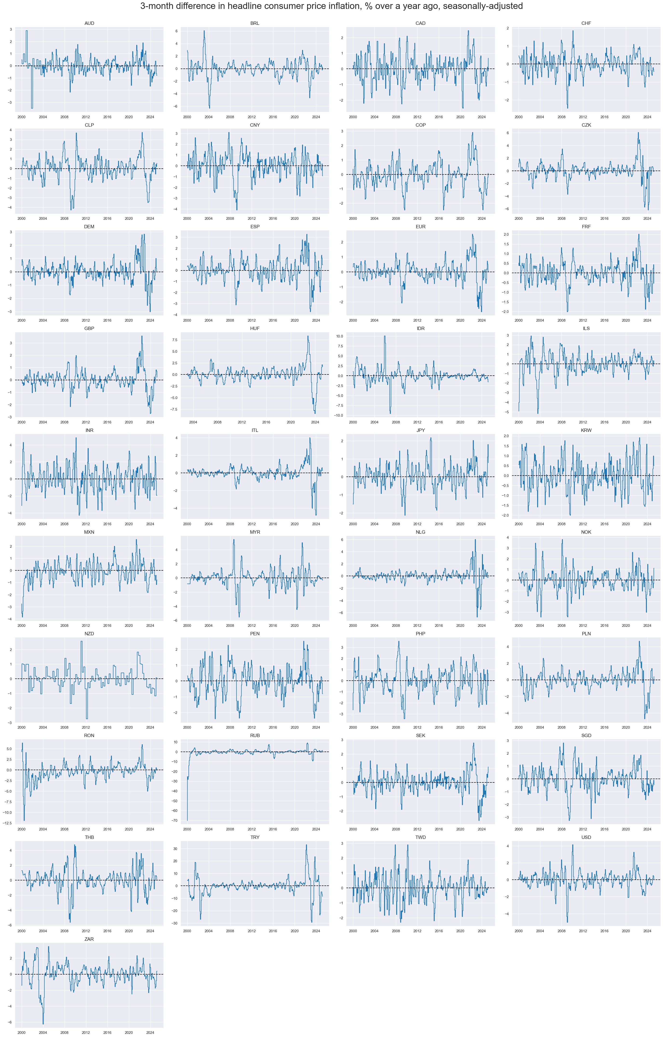
Like in inflation trends and variation, also changes in inflation trends (based on concurrent vintages) and their variations have been widely different acrosss countries.
xcatx = ["CPIH_SA_P1M1ML12_D1M1ML3"]
cidx = cids_exp

msp.view_ranges(
    df,
    xcats=xcatx,
    cids=cidx,
    sort_cids_by="std",
    start="2000-01-01",
    kind="box",
    title="Boxplots for changes in headline consumer price inflation, seasonally-adjusted, since 2000",
    xcat_labels=["3-month difference in 1-year % change"],
    size=(16, 8),
)
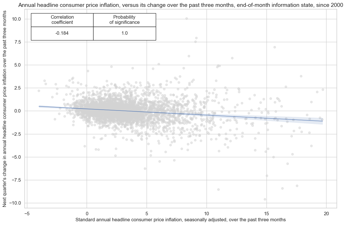
The relationship between the current level of inflation and the change in inflation in the next period tends to be negative, suggesting a straightforward concept: high inflation today may prompt actions by policymakers aimed at reducing inflation in the future.
cr = msp.CategoryRelations(
    df,
    xcats=["CPIH_SA_P1M1ML12", "CPIH_SA_P1M1ML12_D1M1ML3"],
    cids=cids,
    freq="Q",
    lag=1,
    xcat_aggs=["last", "last"],
    xcat_trims=[20,20],
    start="2000-01-01",
)

cr.reg_scatter(
        labels=False,
    coef_box="upper left",
    title = "Annual headline consumer price inflation, versus its change over the past three months, end-of-month information state, since 2000",
    xlab="Standard annual headline consumer price inflation, seasonally adjusted, over the past three months",
    ylab="Next quarter's change in annual headline consumer price inflation over the past three months",
    prob_est="map"
)
xcatx = ["CPIH_SA_P1M1ML12_D1M1ML3"]
cidx = cids_exp


msp.view_timelines(
    df,
    xcats=xcatx,
    cids=cidx,
    start="2000-01-01",
    title="3-month difference in headline consumer price inflation, % over a year ago, seasonally-adjusted",
    title_fontsize=27,
    ncol=4,
    same_y=False,
    all_xticks=True,
)
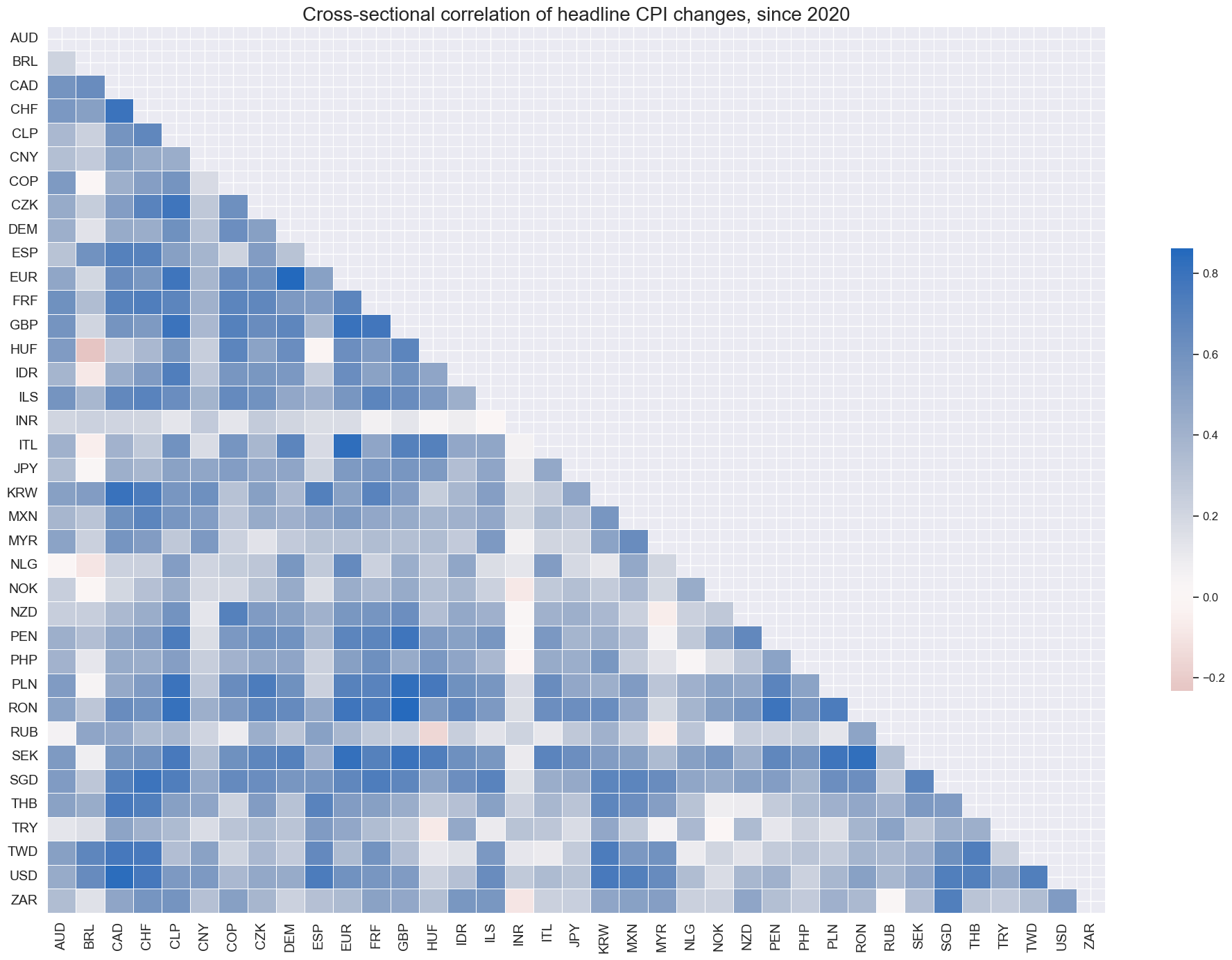
There has been a dominant positive relation between the information states of headline inflation changes across countries. This means published data across currency areas usually signal the same direction of change. Food and energy prices are main driver of this correlation, but not the only. Also, core inflation changes have been positively correlated.
xcatx = "CPIH_SA_P1M1ML12_D1M1ML3"
cidx = cids_exp

msp.correl_matrix(
    df,
    xcats=xcatx,
    cids=cidx,
    title="Cross-sectional correlation of headline CPI changes, since 2020",
    start="2020-01-01",
    size=(20, 14),
)
Shorter-term core inflation trends #
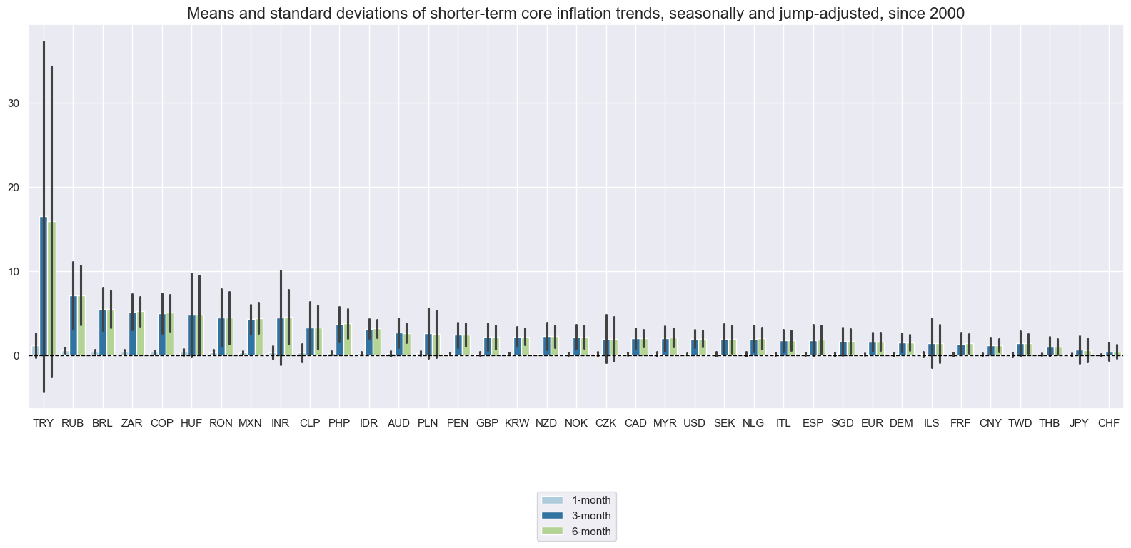
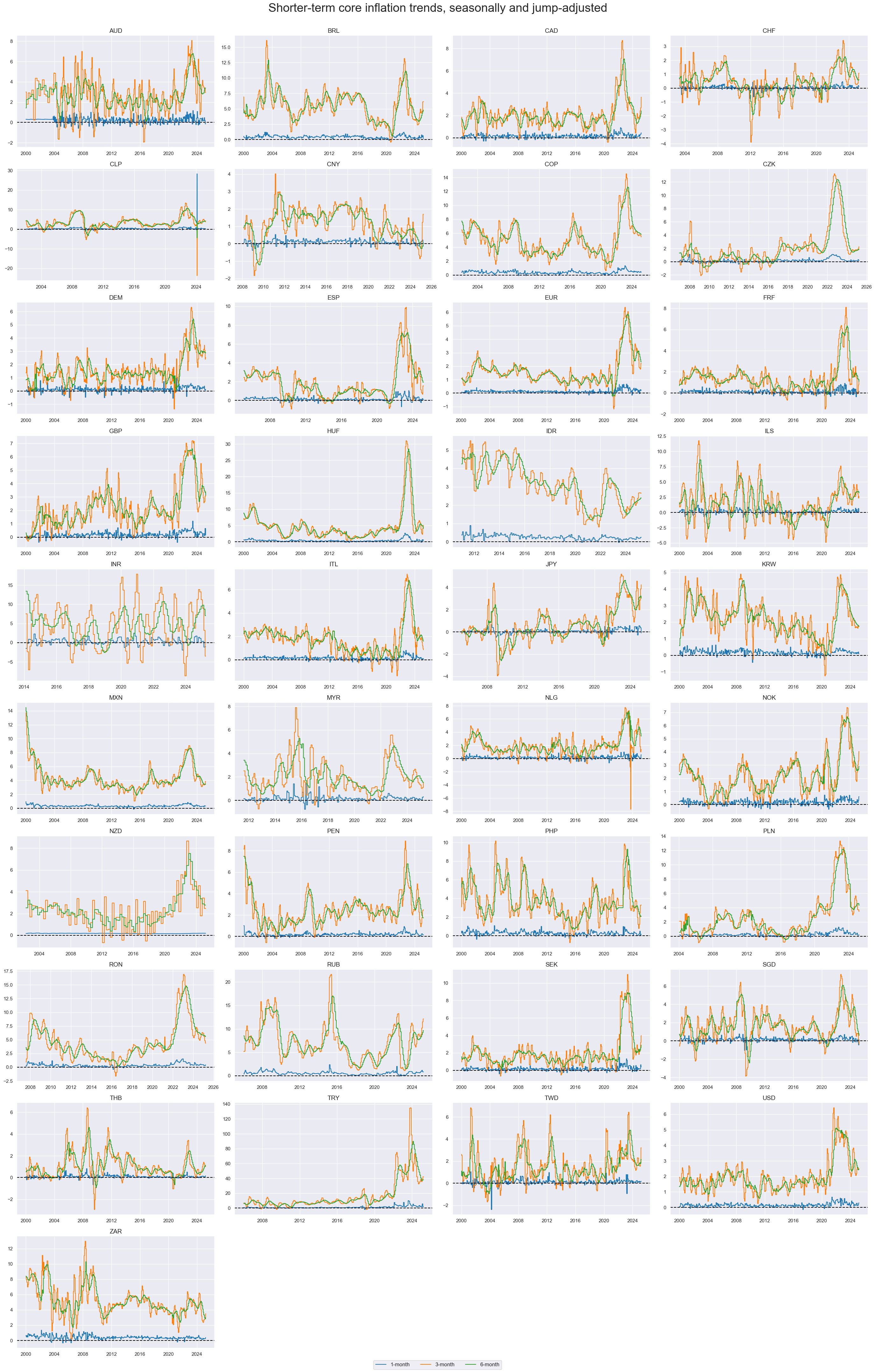
The seasonally and jump-adjusted 6-month over 6-month core CPI trends have been fairly stable trend indicators for most currency areas.
xcatx = ["CPIC_SJA_P1M1ML1","CPIC_SJA_P3M3ML3AR", "CPIC_SJA_P6M6ML6AR"]
cidx = cids_exp

msp.view_ranges(
    df,
    xcats=xcatx,
    cids=cidx,
    sort_cids_by="mean",
    start="2000-01-01",
    title="Means and standard deviations of shorter-term core inflation trends, seasonally and jump-adjusted, since 2000",
    xcat_labels=["1-month","3-month", "6-month"],
    kind="bar",
    size=(16, 8),
)
xcatx = ["CPIC_SJA_P1M1ML1","CPIC_SJA_P3M3ML3AR", "CPIC_SJA_P6M6ML6AR"]
cidx = cids_exp

msp.view_timelines(
    df,
    xcats=xcatx,
    cids=cidx,
    start="2000-01-01",
    title="Shorter-term core inflation trends, seasonally and jump-adjusted",
    title_fontsize=27,
    xcat_labels=["1-month","3-month", "6-month"],
    ncol=4,
    same_y=False,
    all_xticks=True,
)
CPI, using early estimates #
The longer-term pattern of regular CPI inflation and the version with early estimates have naturally been very similar as the two metrics converge on a monthly basis.
For currency areas with regression estimates, such as GBP or PHP, the influence of the early estimate varies over time, in accordance with previous historical experience. This reflects that the predictive regression is sequentially re-estimated in order to avoid any hindsight bias.
xcatx = ["CPIH_SA_P1M1ML12", "CPIHE_SA_P1M1ML12"]
cidx = msm.common_cids(df, xcats=xcatx)

msp.view_timelines(
    df,
    xcats=xcatx,
    cids=cidx,
    start="2000-01-01",
    title="Headline CPI trends, % change over a year ago, information states",
    legend_fontsize=17,
    xcat_labels=["Regular headline CPI", "Using early estimate prior to release"],
    ncol=4,
    same_y=False,
    all_xticks=True,
    legend_ncol=2,
)

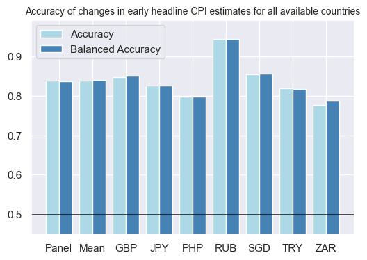
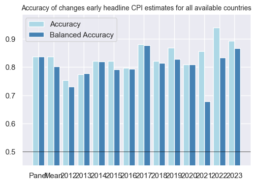
Changes in the early headline inflation indicators (%oya over 3 months) are highly accurate in forecasting standard inflation changes (%oya over 3 months), achieving an accuracy rate of approximately 80% across all available countries.
xcatx = ["CPIH_SA_P1M1ML12_D1M1ML3", "CPIHE_SA_P1M1ML12_D1M1ML3"]
cidx = msm.common_cids(df, xcats=xcatx)

srr = mss.SignalReturnRelations(
    df,
    cids=cids_early,
    sigs=["CPIHE_SA_P1M1ML12_D1M1ML3"],
    sig_neg=[False],
    rets=["CPIH_SA_P1M1ML12_D1M1ML3"],
    freqs=["M"],
    start="2012-01-01",
    end="2023-12-01"
)

srr.accuracy_bars(title = "Accuracy of changes in early headline CPI estimates for all available countries", size = (6,4), title_fontsize = 10)
srr.accuracy_bars(type="years", title = "Accuracy of changes early headline CPI estimates for all available countries", size = (6,4), title_fontsize = 10)
Importance #
Research links #
Importance of core and headline inflation measures:
“The price stability objective of the Eurosystem is to maintain annual rates of headline HICP (Harmonised Index of Consumer Prices) inflation at below, but close to, 2% over the medium term.” ECB Economic Bulletin, Issue 4/2018 . “Since the 1970s, the primary measure of core at the Federal Reserve has been the inflation rate excluding food and energy (XFE inflation)” IMF WP/22/208 .
Inflation and asset prices:
“Changes in the general level of prices and inflation have profound effects on asset prices. There are several reasons for these effects… including supply shocks that reduce wealth and raise prices, and tax effects of inflation that arise from a lack of full indexation of the tax system. Inflation has had large effects on asset prices in the United States, especially during the Great Inflation from 1965 to 1984.” John Tatom
On inflation and real interest rates:
“The co-movement between inflation and economic activity is an important determinant of real interest rates over time and across countries…For advanced economies, periods with more procyclical inflation are associated with lower real rates…when there is no risk of default on government debt.” Hur, Kondo and Perri
On stocks returns and monetary policy frameworks:
“ the stock return-inflation relation differ when the central banks target different nominal anchors. They are two extreme cases of whether monetary policy responds directly to inflation or not. The conjecture is that if monetary policy solely focuses on stabilizing the exchange rate, policy cyclicality will not change how real stock returns react to inflation. On the other hand, if monetary policy targets inflation only, policy cyclicality will have strong and unintended consequences on market responses to inflation.” IMF Working Paper WP 21/219
Inflation expectations and equity/CDS:
“A downward shift in expected inflation increases equity valuations and credit default risk at the same time. The reason for this is ‘nominal stickiness’. A slowdown in consumer prices reduces short-term interest rates but does not immediately reduce earnings growth by the same rate, thus increasing the discounted present value of future earnings. At the same time, a downward shift in expected inflation increases future real debt service and leverage of firms and increases their probability of default. This theory is supported by the trends in U.S. markets since 1970. It would principally argue for strategic relative equity-CDS positions inversely to the broad trend in expected inflation.” Macrosynergy .
Early empirical research found, that “… common stock returns were negatively related to the expected component of the inflation rate, and probably also to the unexpected component” (for the period 1953-71) Eugene F. Fama and G. William Schwert .
“Classical theories of monetary economics predict that real stock returns are negatively correlated with inflation when monetary policy is countercyclical.” IMF Working Paper WP/21/219 . For a dedicated post using inflation as a predictor of equity returns, see here
“The results of cointegration regression show that inflation rates are negatively associated with stock prices, the real interest rates and stock prices are positively associated, changes in real interest rates and inflation rates Granger cause significant changes in stock prices.” Tarek Eldomiaty et. al
Inflation expectations and fixed income returns:
“Few would dispute that long-lasting episodes of high inflation pose a major risk for investors in nominal bonds, eroding their ability to consume out of fixed dollar payoffs.” Anna Cieslak and Carolin Pflueger
“… overriding conclusion from…” (current empirical research is that )” … persistent (trend) inflation shocks are costly and induce significant risk premia in both stocks and bonds.” Anna Cieslak1,2,3 and Carolin Pflueger
Inflation and FX returns:
“… for inflation targeting countries, bad news for inflation is good news for the exchange rate… “ R Clarida and D Waldman, IMF
“High rates normally lead to an appreciation of the currency, as foreign investors seek higher returns and increase their demand for the currency.” IMF publication . To empirically examine this proposition, we construct excess inflation metrics using changes in headline inflation and 6-month/6-month percentage changes. Subsequently, we compare these metrics with relative 1-month foreign exchange (FX) forward returns, focusing on positions established with 10% volatility targets.
Correlation of inflation for OECD countries
“Inflations of 22 OECD countries have a common factor that accounts for nearly 70% of their variance.” Matteo Ciccarelli and Benoît Mojon .
“…the contribution of global shocks to domestic inflation variation was larger in advanced economies and countries with higher trade and financial openness, fixed exchange rate regimes, and greater reliance on commodity imports.” Inflation in Emerging and Developing Economies: Evolution, Drivers, and Policies
“…existing estimates indicate that inflation synchronization is more pronounced among advanced economies than in emerging market economies”, Banco de México, Working Paper N° 2022-15 .
“In an integrated global economy, inflation may co-move across economies for two reasons: either because of common shocks that hit all countries simultaneously, even if not symmetrically, such as the oil shocks of the 1970s, or because of idiosyncratic or regional shocks, such as the Asian financial crisis of 1997 or the euro area sovereign debt crisis of 2012, that are large enough to affect output and prices worldwide. Today, we are seeing both forces at work.” Isabel Schnabel, Member of the Executive Board of the ECB .
“…the pandemic, and more recently Russia’s invasion of Ukraine are providing tangible evidence in favour of … “globalisation of inflation” hypothesis”, Speech by Isabel Schnabel, Member of the Executive Board of the ECB
Inflation matters for financial returns due to two main reasons:
“For investors, returns on investments should be at least as high as the inflation rate. Otherwise, their investments are losing money even if they gain in dollar value. Similarly, individuals should ensure that their salaries keep pace with inflation; otherwise, they are losing buying power.” Investopedia . Higher inflation means higher demanded returns.
“Central banks use interest rates to control demand and inflation. If inflation is high, they raise their target for short-term interest rates… Since 2021… high inflation has pushed many central banks to start raising interest rates, which threatens to slow global growth” Walter Frick
Consumer price inflation trends indicators are used in many Macrosynergy’ posts and accompanying notebooks:
Empirical clues #
This section examines the proof of concept, presenting a stylized Profit and Loss (PnL) profile for a collection of trading signals based on inflation. The trading signals involve simple inflation metrics based on excess inflation. Excess inflation pertains to consumer price trends that exceed the predefined inflation target. Our focus in this analysis extends to potential asset classes deemed suitable for consideration:
-
generic government bond returns,
-
directional duration returns,
-
relative duration returns,
-
equity returns,
-
directional FX returns, and
-
relative FX returns.
# The first step is to calculate the effective inflation target for each country. This is done by taking the maximum of the inflation target and 2%.

scols=["cid", "xcat", "real_date", "value"]
dfx = df[scols].copy().sort_values(["cid", "xcat", "real_date"])
dfx["ticker"] = dfx["cid"] + "_" + dfx["xcat"]


dfa = msp.panel_calculator(dfx, ["INFTEBASIS = INFTEFF_NSA.clip(lower=2)"], cids=cids) # `INFTEBASIS` is  the maximum of
# the effective inflation target and 2.
dfx = msm.update_df(dfx, dfa)

# The second step is to calculate the relative deviations of the inflation rate from the effective inflation target.

sigx = [
    "CPIH_SA_P1M1ML12",
    "CPIH_SJA_P6M6ML6AR",
    "CPIH_SJA_P3M3ML3AR",
    "CPIC_SA_P1M1ML12",
    "CPIC_SJA_P3M3ML3AR",
    "CPIC_SJA_P6M6ML6AR"
]

for inf in sigx:
    calcs = [
        f"{inf}vIET = ( {inf} - INFTEFF_NSA ) / INFTEBASIS",
    ]

    dfa = msp.panel_calculator(dfx, calcs=calcs, cids=cids) # This scaling of the excess inflation is a standard procedure to make the effects of inflation changes comparable across the range of
    # of high and low inflation countries.

    dfx = msm.update_df(dfx, dfa)

# The next step is calculation of the simple average of the three excess inflation metrics:

calcs = []
for cp in ["CPIH", "CPIC"]:
    for v in ["vIET"]:
        calc = f"{cp}_SA_PALL{v} = ( {cp}_SA_P1M1ML12{v} + {cp}_SJA_P6M6ML6AR{v} + {cp}_SJA_P3M3ML3AR{v} ) / 3"
        calcs += [calc]

dfa = msp.panel_calculator(dfx, calcs, cids=cids)
dfx = msm.update_df(dfx, dfa)

# Lastly we calculate simple averages of USD-EUR inflation metrics:

calcs = [
    "iUSD_iEUR_CPIH_SA_PALLvIET = ( iUSD_CPIH_SA_PALLvIET +  iEUR_CPIH_SA_PALLvIET ) / 2",   # USD-EUR inflation
    "iUSD_iEUR_CPIH_SJA_P6M6ML6ARvIET = ( iUSD_CPIH_SJA_P6M6ML6ARvIET +  iEUR_CPIH_SJA_P6M6ML6ARvIET ) / 2",
    "iUSD_CPIC_SJA_P6M6ML6ARvIET = iUSD_CPIC_SJA_P6M6ML6ARvIET"]

dfa = msp.panel_calculator(dfx, calcs, cids=cids)
dfx = msm.update_df(dfx, dfa)
Inflation and government bond returns #
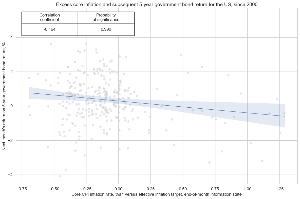
In the United States, core PCE inflation is the key price indicator for monetary policy. In the presence of some rational inattention to price trends and their implication for Federal Reserve words and actions, we would expect core inflation above target to predict subsequent Treasure bond returns negatively. Indeed the relation between excess core inflation and subsequent 5-year IRS bomd returns has been negative and significantly so, at a weekly, monthly, and quarterly frequency.
cr_bond = msp.CategoryRelations(
    dfx,
    xcats=["CPIC_SJA_P6M6ML6ARvIET", "GB05YR_NSA"],
    cids=["USD"],
    freq="M",
    lag=1,
    xcat_aggs=["last", "sum"],
    start="1990-01-01",
)

cr_bond.reg_scatter(
    title="Excess core inflation and subsequent 5-year government bond return for the US, since 2000",
    labels=False,
    coef_box="upper left",
    xlab="Core CPI inflation rate, %ar, versus effective inflation target, end-of-month information state",
    ylab="Next month's return on 5-year government bond return, %",
    prob_est="map"
)
Inflation as a predictor of IRS returns #
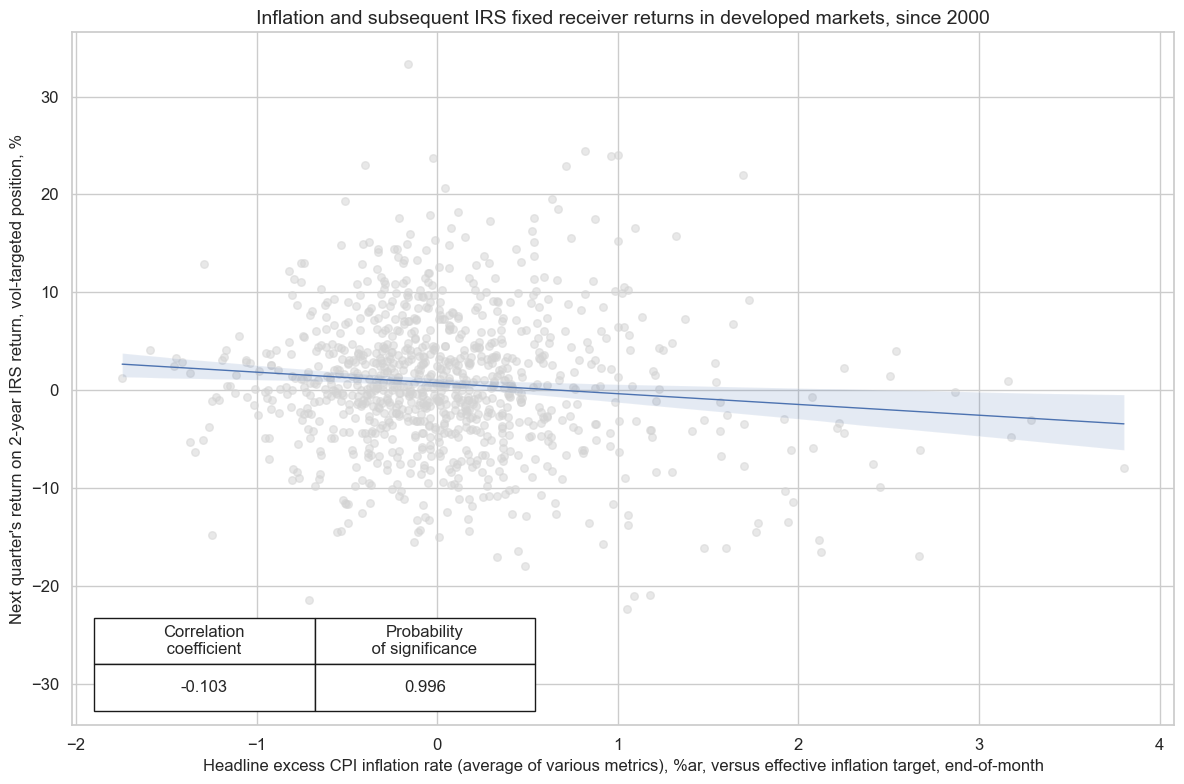
Excess inflation, above effective targets, has also negatively predicted interest rate swap reciver returns, at various frequencies and tenors. Generally, predictive correlation has been stronger for shorter-maturity contracts.
cr_du = msp.CategoryRelations(
    dfx,
    xcats=["CPIH_SA_PALLvIET", "DU02YXR_VT10"],
    cids=cids_dmca,
    freq="Q",
    lag=1,
    xcat_aggs=["last", "sum"],
    start="2000-01-01",
)

cr_du.reg_scatter(
    title="Inflation and subsequent IRS fixed receiver returns in developed markets, since 2000",
    labels=False,
    coef_box="lower left",
    xlab="Headline excess CPI inflation rate (average of various metrics), %ar, versus effective inflation target, end-of-month",
    ylab="Next quarter's return on 2-year IRS return, vol-targeted position, %",
    prob_est="map"
)
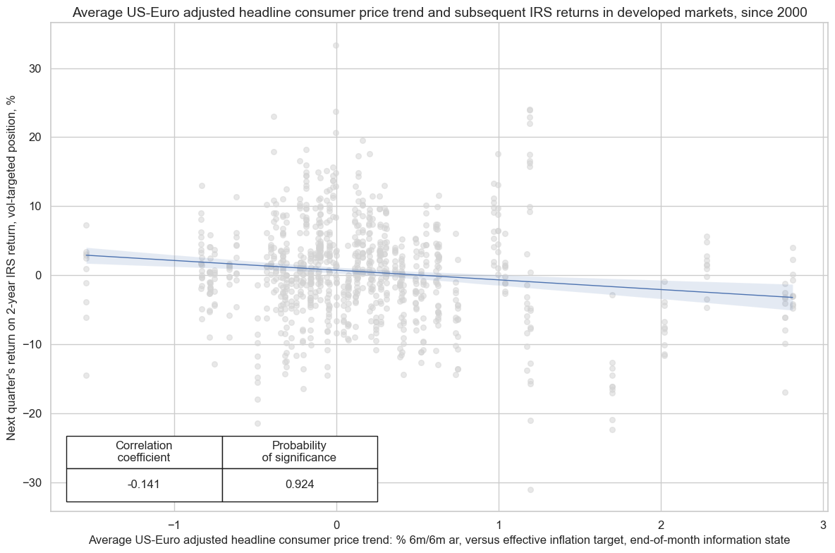
The negative predictive correlation between inflation and fixed receiver contract returns has been even stronger if one uses average U.S. and euro-area excess inflation as predictors for all developed countries, testifying to the dominance of these two economic areas and central banks for global interest rate markets. However, statistical significance has been a bit lower because the choice of communal predictors means less cross-country variation and an inability to draw lessons from cross-country inflation differences.
cr_du = msp.CategoryRelations(
    dfx,
    xcats=["iUSD_iEUR_CPIH_SJA_P6M6ML6ARvIET", "DU02YXR_VT10"],
    cids=cids_dmca,
    freq="Q",
    lag=1,
    xcat_aggs=["last", "sum"],
    start="2000-01-01",
)

cr_du.reg_scatter(
    title="Average US-Euro adjusted headline consumer price trend and subsequent IRS returns in developed markets, since 2000",
    labels=False,
    coef_box="lower left",
    xlab="Average US-Euro adjusted headline consumer price trend: % 6m/6m ar, versus effective inflation target, end-of-month information state",
    ylab="Next quarter's return on 2-year IRS return, vol-targeted position, %",
    prob_est="map"
)
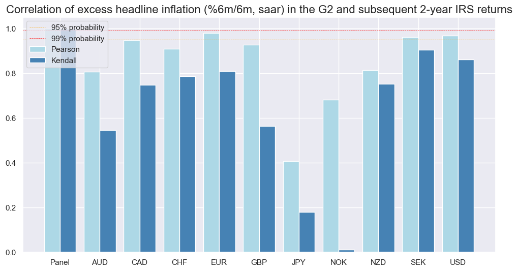
The predictive correlation of excess inflation in the G2 and subsequent monthly IRS receiver returns has been negative across all developed markets. This has not been the case for predictive correlations between local inflation: In Switzerland and Japan, the relation between inflation and subsequent receiver returns has been slightly positive. Presumably, in deflationary economies with zero or sub-zero policy rates inflation trends did little to affect short-term rates expectations over the past decades.
srr_du = mss.SignalReturnRelations(
    dfx,
    cids=cids_dmca,
    sigs= "iUSD_iEUR_CPIH_SJA_P6M6ML6ARvIET",
    sig_neg=[True],
    rets=["DU02YXR_VT10"],
    freqs=["M"],
    start="2000-01-01",
)

srr_du.correlation_bars(
    title = "Correlation of excess headline inflation (%6m/6m, saar) in the G2 and subsequent 2-year IRS returns",
    size=(12, 6)
)
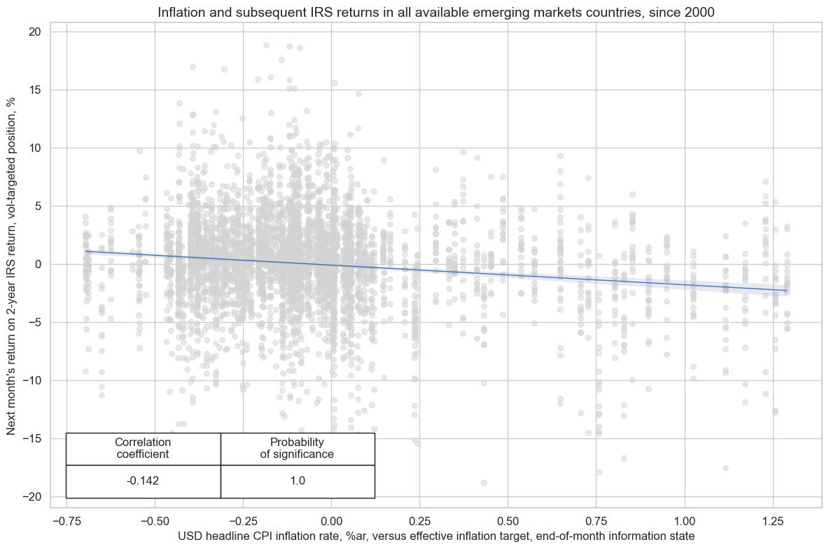
U.S. and euro area excess inflation also predicted emerging markets’ rate performances negatively. The predictive power has been stronger for the U.S. alone since the U.S. dollar is the dominant EM funding currency. Typically, high inflation in the G2 supports policy tightening in the large financial markets, which subsequently puts pressure on global capital flows and emerging market currencies, which then necessitates higher local rates in EM countries.
# we take out bad-data return periods for fixed income markets
filt_try = (dfx["cid"] == "TRY") & (dfx["real_date"] > pd.to_datetime("2022-08-01"))
dfx.loc[filt_try, "value"] = np.nan

cr_du = msp.CategoryRelations(
    dfx,
    xcats=["iUSD_CPIC_SJA_P6M6ML6ARvIET", "DU02YXR_VT10"],
    cids = cids_em,
    freq="M",
    lag=1,
    xcat_aggs=["last", "sum"],
    xcat_trims=[20,20],
    start="2000-01-01",
)

cr_du.reg_scatter(
    title="Inflation and subsequent IRS returns in all available emerging markets countries, since 2000",
    labels=False,
    coef_box="lower left",
    xlab="USD headline CPI inflation rate, %ar, versus effective inflation target, end-of-month information state",
    ylab="Next month's return on 2-year IRS return, vol-targeted position, %",
    prob_est="map",

)
DU02YXR_VT10 misses: ['PEN', 'PHP', 'RON'].
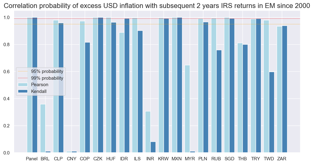
The negative predictive relation between U.S. excess inflation and EM fixed IRS receivers has been significant individually in most markets. Also, the predictive relation was negative across currency areas, with China being the only exception.
srr_du = mss.SignalReturnRelations(
    dfx,
    cids=cids_em,
    sigs="iUSD_CPIC_SJA_P6M6ML6ARvIET",
    sig_neg=True,
    rets="DU02YXR_VT10",
    freqs=["M"],
    start="2000-01-01",
)

srr_du.correlation_bars(
    title="Correlation probability of excess USD inflation with subsequent 2 years IRS returns in EM since 2000",
    size=(12, 6),
)
Inflation as a predictor of relative IRS returns #
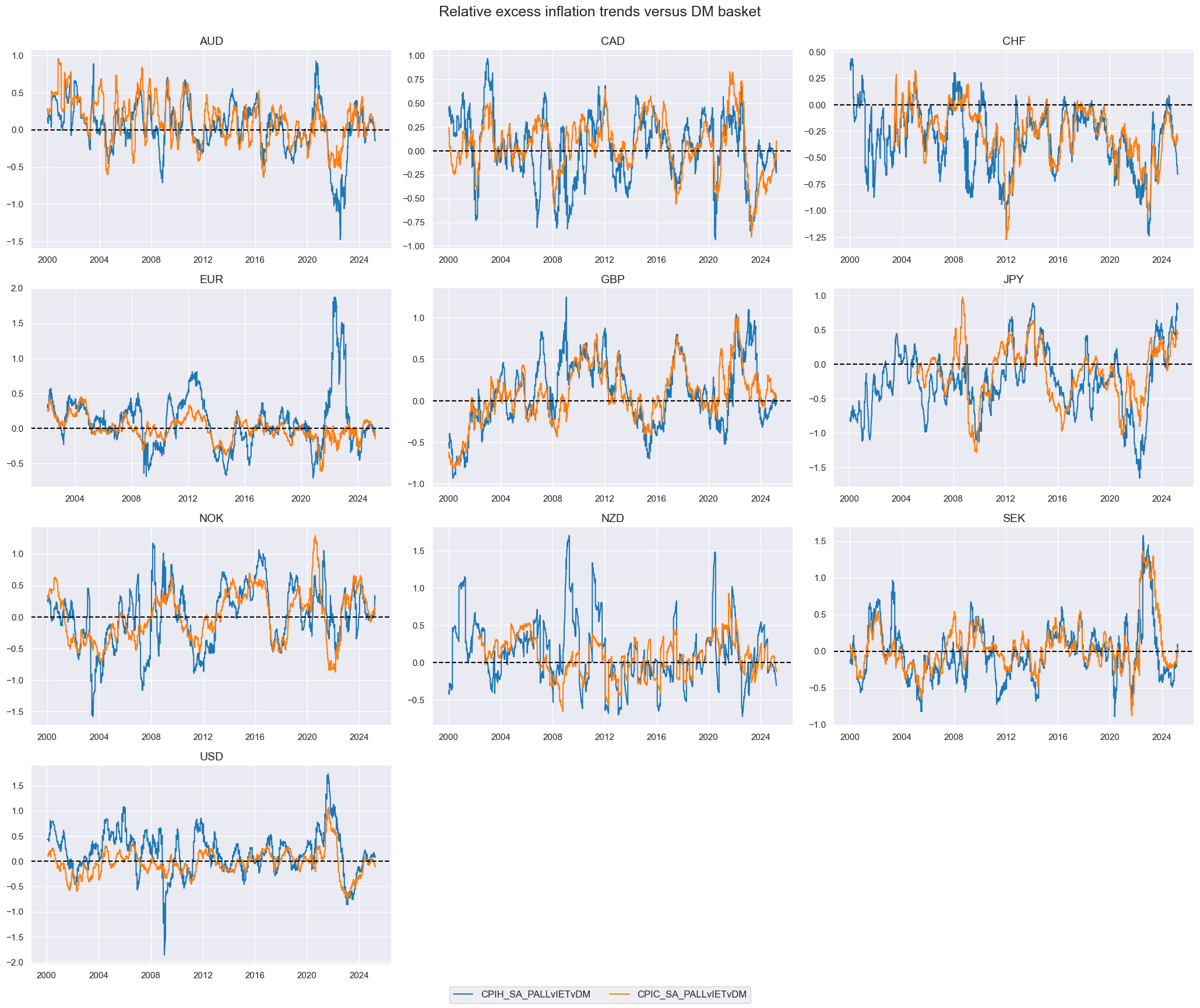
Here, we define relative headline or core inflation as the average (%oya, %6m/6m, saar, %3m/3m, saar) excess inflation rate of one (developed market) currency area versus the average of all currency areas.
dfa = msp.make_relative_value(
    dfx,
    xcats=["DU02YXR_VT10", "DU05YXR_VT10", "CPIH_SA_PALLvIET", "CPIC_SA_PALLvIET"],
    cids=cids_dmca,
    postfix="vDM",
)
dfx = msm.update_df(dfx, dfa)
xcatx = ["CPIH_SA_PALLvIETvDM", "CPIC_SA_PALLvIETvDM"]


msp.view_timelines(
    dfx,
    xcats=xcatx,
    cids=cids_dmca,
    ncol=3,
    cumsum=False,
    start="2000-01-01",
    same_y=False,
    all_xticks=True,
    title="Relative excess inflation trends versus DM basket",
    xcat_labels=None,
)
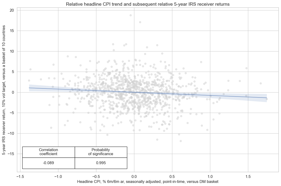
Relative excess inflation, whether headline or core, has also been negatively and significantly correlated with subsequent IRS returns, across 2-year and 5-year tenors and for weekly, monthly, and quarterly frequencies.
crx = msp.CategoryRelations(
    dfx,
    xcats=["CPIH_SA_PALLvIETvDM", "DU05YXR_VT10vDM"],
    cids=cids_dmca,
    freq="Q",
    lag=1,
    xcat_aggs=["last", "sum"],
    start="2000-01-01",
    xcat_trims=[None, None],
)
crx.reg_scatter(
    labels=False,
    coef_box="lower left",
    xlab="Headline CPI, % 6m/6m ar, seasonally adjusted, point-in-time, versus DM basket",
    ylab="5-year IRS receiver return, 10% vol target, versus a basket of 10 countries",
    title="Relative headline CPI trend and subsequent relative 5-year IRS receiver returns",
    size=(12, 8),
    prob_est="map",
)
Inflation as a predictor of equity returns #
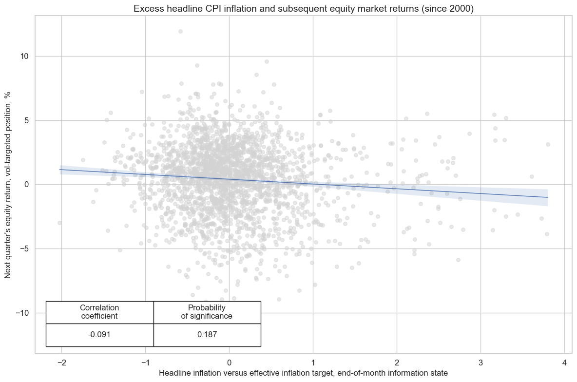
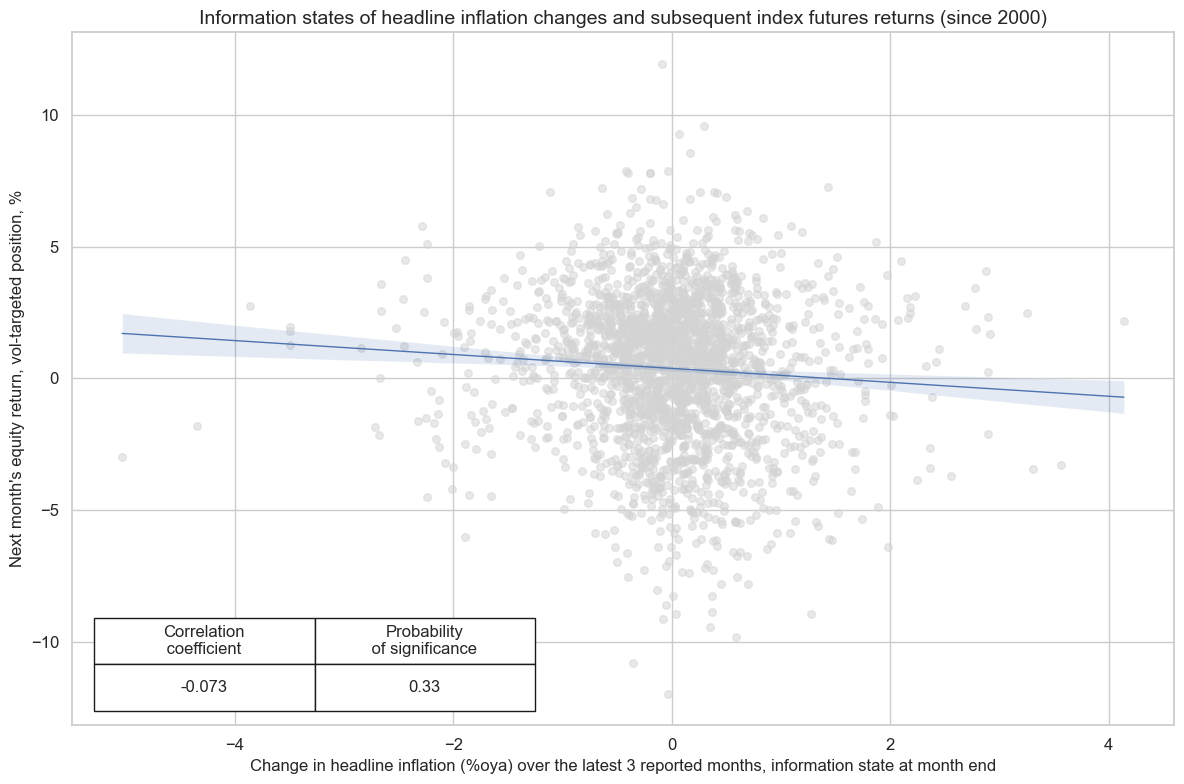
Excess inflation and changes in inflation have been negatively correlated with subsequent equity index future returns since 2000 for developed countries. However, the relations have not (yet) been statistically significant, according to the Macrosynergy panel test. The apparent negative correlation of the pooled dataset in a scatterplot is actually misleading. This is because most of the negative relation comes from 1 or 2 episodes of accelerating and slowing CPIs around the great financial crisis and the COVID-19 pandemic, which are (pseudo-) replicated across all markets. The relation has been consistent, and relative inflation differentials have not strongly predicted relative equity returns.
cr_eq = msp.CategoryRelations(
    dfx,
    xcats=["CPIH_SA_PALLvIET", "EQXR_VT10"],
    cids = cids_dmca,
    freq="M",
    lag=1,
    xcat_aggs=["last", "sum"],
    start="2000-01-01",
)

cr_eq.reg_scatter(
    title="Excess headline CPI inflation and subsequent equity market returns (since 2000)",
    labels=False,
    coef_box="lower left",
    xlab="Headline inflation versus effective inflation target, end-of-month information state",
    ylab="Next quarter's equity return, vol-targeted position, %",
    prob_est="map"
)
EQXR_VT10 misses: ['NOK', 'NZD'].
cr_eq = msp.CategoryRelations(
    dfx,
    xcats=["CPIH_SA_P1M1ML12_D1M1ML3", "EQXR_VT10"],
    cids = cids_dmca,
    freq="M",
    lag=1,
    xcat_aggs=["last", "sum"],
    start="2000-01-01",
)

cr_eq.reg_scatter(
    title="Information states of headline inflation changes and subsequent index futures returns (since 2000)",
    labels=False,
    coef_box="lower left",
    xlab="Change in headline inflation (%oya) over the latest 3 reported months, information state at month end",
    ylab="Next month's equity return, vol-targeted position, %",
    prob_est="map"
)
EQXR_VT10 misses: ['NOK', 'NZD'].
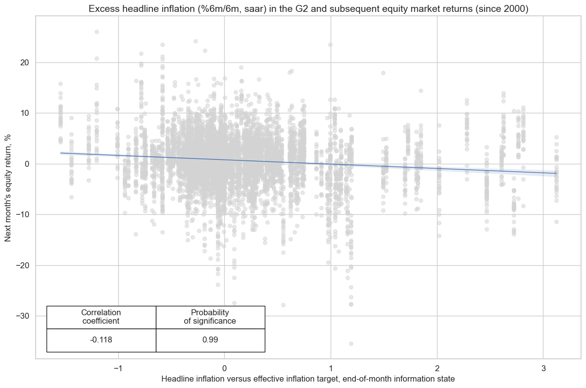
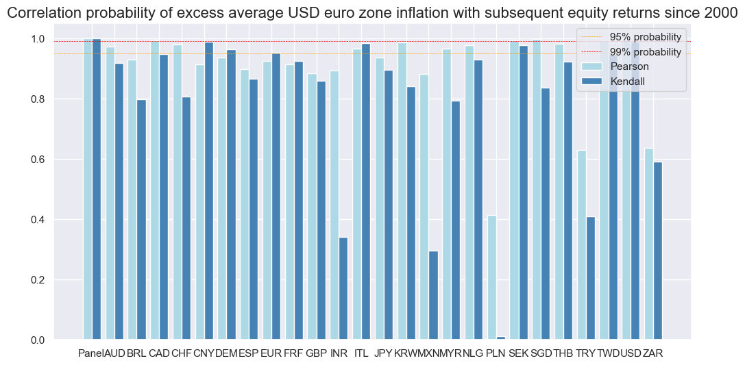
Excess average USD euro zone inflation is negatively correlated with subsequent equity index future returns since 2000 using all available countries. This relation has been statistically significant, according to the Macrosynergy panel test, and consistent. This suggests that inflation has been an important predictor of equity returns in the large markets and - hence - globally. However, inflation differentials across countries have not been a powerful predictor.
cids_EQXR_NSA = dfx[dfx["xcat"] == "EQXR_NSA"]["cid"].unique()
cids_iUSD_iEUR_CPIH_SJA_P6M6ML6ARvIET = dfx[dfx["xcat"] == "iUSD_iEUR_CPIH_SJA_P6M6ML6ARvIET"]["cid"].unique()
common_cids = np.intersect1d(cids_EQXR_NSA, cids_iUSD_iEUR_CPIH_SJA_P6M6ML6ARvIET)

cr_eq = msp.CategoryRelations(
    dfx,
    xcats=["iUSD_iEUR_CPIH_SJA_P6M6ML6ARvIET", "EQXR_NSA"],
    cids = common_cids,
    freq="M",
    lag=1,
    xcat_aggs=["last", "sum"],
    start="2000-01-01",
)

cr_eq.reg_scatter(
    title="Excess headline inflation (%6m/6m, saar) in the G2 and subsequent equity market returns (since 2000)",
    labels=False,
    coef_box="lower left",
    xlab="Headline inflation versus effective inflation target, end-of-month information state",
    ylab="Next month's equity return, %",
    prob_est="map"
)
srr_eq = mss.SignalReturnRelations(
    dfx,
    cids=list(dfx[dfx["xcat"] == "EQXR_NSA"]["cid"].unique()),
    sigs= "iUSD_iEUR_CPIH_SJA_P6M6ML6ARvIET",
    sig_neg=[True],
    rets=["EQXR_NSA"],
    freqs=["M"],
    start="2000-01-01",
)


srr_eq.correlation_bars(
    title="Correlation probability of excess average USD euro zone inflation with subsequent equity returns since 2000",
    size=(12, 6),
)
Inflation as a predictor of directional FX returns #
The main hypothesis for the relation between inflation and FX forward returns is that higher excess inflation triggers tighter monetary policy and a strong currency. For this to hold logically, we must look at excess inflation differentials of various currencies against their natural benchmarks, against the most frequently quoted base currency. This is the dollar for most, but the euro for CHF, CZK, HUF, NOK, PLN, RON, SEK. and both dollar and euro for GBP, RUB, TRY.
The computed excess inflation ratios will be designated with the suffix
_vBM
cids_fx = list(set(cids) - set(["EUR", "USD"]))
cids_eur = ["CHF", "CZK", "HUF", "NOK", "PLN", "RON", "SEK"]  # trading against EUR
cids_eud = ["GBP", "RUB", "TRY"]  # trading against EUR and USD
cids_usd = list(set(cids_fx) - set(cids_eur + cids_eud))  # trading against USD


xcatx = ["CPIH_SJA_P6M6ML6ARvIET", "CPIC_SJA_P6M6ML6ARvIET", "CPIC_SA_P1M1ML12_D1M1ML3", "CPIC_SJA_P3M3ML3AR", "CPIH_SJA_P3M3ML3AR"]

for xc in xcatx:
    calc_eur = [f"{xc}vBM = {xc} - iEUR_{xc}"]
    calc_usd = [f"{xc}vBM = {xc} - iUSD_{xc}"]
    calc_eud = [f"{xc}vBM = {xc} - 0.5 * ( iEUR_{xc} + iUSD_{xc} )"]

    dfa_eur = msp.panel_calculator(
        dfx,
        calcs=calc_eur,
        cids=cids_eur,
    )
    dfa_usd = msp.panel_calculator(
        dfx,
        calcs=calc_usd,
        cids=cids_usd,
    )
    dfa_eud = msp.panel_calculator(
        dfx,
        calcs=calc_eud,
        cids=cids_eud,
    )

    dfa = pd.concat([dfa_eur, dfa_usd, dfa_eud])
    dfx = msm.update_df(dfx, dfa)
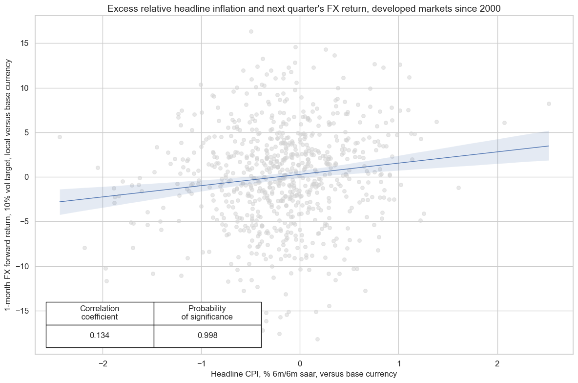
Indeed, the relationship between relative excess inflation rates and subsequent FX forward returns has been strongly and significantly positive for developed market currencies at various frequencies.
cids_dmfx =(list(set(cids_dmca) - set(["USD", "EUR"]))) # DM currencies excluding USD, EUR

crx = msp.CategoryRelations(
    dfx,
    xcats=["CPIH_SJA_P6M6ML6ARvIETvBM", "FXXR_VT10"],
    cids=cids_dmfx,
    freq="Q",
    lag=1,
    xcat_aggs=["last", "sum"],
    xcat_trims=[20,20 ],
    start="2000-01-01",


)
crx.reg_scatter(
    labels=False,
    coef_box="lower left",
    xlab="Headline CPI, % 6m/6m saar, versus base currency",
    ylab="1-month FX forward return, 10% vol target, local versus base currency",
    title="Excess relative headline inflation and next quarter's FX return, developed markets since 2000",
    prob_est="map",
)
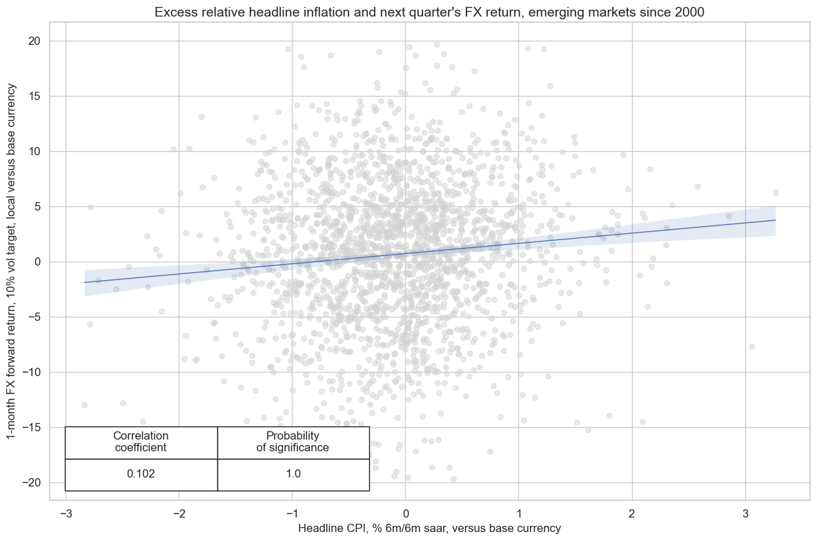
The positive relationship between excess inflation differentials and subsequent FX returns has been similarly strong and significant for emerging markets.
crx = msp.CategoryRelations(
    dfx,
    xcats=["CPIH_SJA_P6M6ML6ARvIETvBM", "FXXR_VT10"],
    cids=cids_em,
    freq="Q",
    lag=1,
    xcat_aggs=["last", "sum"],
    xcat_trims=[20,20 ],
    start="2000-01-01",


)
crx.reg_scatter(
    labels=False,
    coef_box="lower left",
    xlab="Headline CPI, % 6m/6m saar, versus base currency",
    ylab="1-month FX forward return, 10% vol target, local versus base currency",
    title="Excess relative headline inflation and next quarter's FX return, emerging markets since 2000",
    prob_est="map",
)
Inflation as a predictor of relative FX returns #
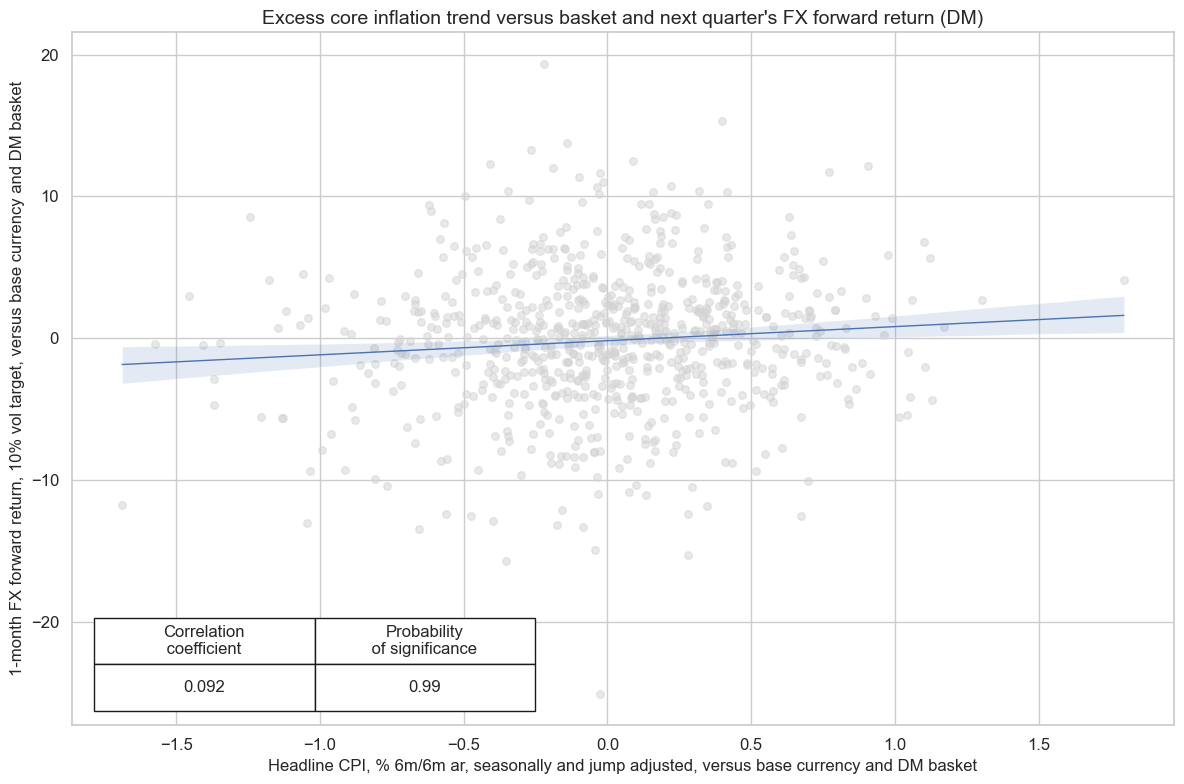
There has also been a strong “double relative” relation between excess inflation, against base currency and a basket of currencies, and FX forward returns, again against base and against a basket of developed market currencies. This predictive relation is valuable because it allows creating a more diversified FX portfolio and reduces the dominant influence of dollar and euro against all other currencies.
dfa = msp.make_relative_value(
    dfx, xcats=["CPIH_SJA_P6M6ML6ARvIETvBM", "FXXR_VT10"], cids=cids_dmfx, postfix="vDM"
)
dfx = msm.update_df(dfx, dfa)


crx_fxrel = msp.CategoryRelations(
    dfx,
    xcats=["CPIH_SJA_P6M6ML6ARvIETvBMvDM", "FXXR_VT10vDM"],
    cids=cids_dmfx,
    freq="Q",
    lag=1,
    xcat_aggs=["last", "sum"],
    start="2000-01-01",
    xcat_trims=[10, 30],
)
crx_fxrel.reg_scatter(
    labels=False,
    coef_box="lower left",
    xlab="Headline CPI, % 6m/6m ar, seasonally and jump adjusted, versus base currency and DM basket",
    ylab="1-month FX forward return, 10% vol target, versus base currency and DM basket",
    title="Excess core inflation trend versus basket and next quarter's FX forward return (DM)",
    prob_est="map",
)
Appendices #
Appendix 1: Volatile component exclusions from core CPI calculations #
Core CPI refers to a CPI that excludes volatile price components according to preferred local convention. The excluded items are as follows:
-
AUD: fruit, vegetables and automotive fuel.
-
BRL: fuel for domestic and for automobile use and 10 items of the food and beverages group.
-
CAD: eight of the most volatile components identified by the Bank of Canada, which are fruit, fruit preparations and nuts, vegetables and vegetable preparations, mortgage interest cost, natural gas, fuel oil and other fuels, gasoline, inter-city transportation, and tobacco products and smokers’ supplies.
-
CHF: food, beverages, tobacco, seasonal products, energy and fuel.
-
CLP: food and energy/ fruit, fresh vegetables and fuel.
-
CNY: food and energy.
-
COP: basic expenses which recorded the largest price volatility and represents 20% of the CPI basket.
-
CZK: effects of tax adjustments and changes in regulated prices and other administrative measures.
-
EUR: food and energy.
-
GBP: energy, food, alcohol and tobacco.
-
HUF: non-processed food items, electricity gas and other fuels, motor fuels and oils, pharmaceutical products that are reimbursed by the social security, services prices thatare centrally determined by authorities.
-
IDR: volatile foods and administered prices, such as subsidized fuel, electricity rates and transportation fares.
-
ILS: housing, fruits and vegetables.
-
INR: food & non-alcholic beverages (JPMaQS calculation).
-
JPY: food (ex alcoholic beverages) and energy/ fresh food.
-
KRW: food & energy.
-
MXN: all that is not in the ‘subyacente’ component is composed by goods and services for which the variation in prices is caused by market conditions.
-
MYR: food.
-
NOK: tax effects and energy products/ electricity.
-
NZD: food, household energy and vehicle fuels.
-
PEN: food and energy.
-
PHP: food.
-
PLN: food and energy.
-
RON: vegetables, fruit, eggs, fuels and administered prices/ administered prices and highly volatile prices (vegetables, fruit, eggs, fuels).
-
RUB: fruits and vegetables, fuel and administrative prices.
-
SEK: energy.
-
SGD: accommodation and private transport.
-
THB: raw food and energy.
-
TRY: energy, food, all beverages, tobacco products and gold.
-
TWD: fruits, vegetables and energy.
-
USD: food and energy.
-
ZAR: food, non-alcoholic beverages, petrol and energy.
For the explanation of currency symbols, which are related to currency areas or countries for which categories are available, please view the subsequent appendix.
Appendix 2: Early CPI estimates #
JPMaQS employs two methods for estimating monthly CPI values prior to the official release for a month.
The first is used when the early indicator is a broad CPI-like index. In this case the estimated CPI is simply the monthly change ratio of the early indicator (EI) times the latest available official CPI.
The second method is applied when the early indicator is a narrower subset of the CPI or a single price. In this case we first run rolling regressions of changes in annual rates in early CPI on concurrent changes in the early indicator. In a case of negative coefficent we set \(\beta_t\) equal to zero.
Then we use the estimated coefficient based on past history and the change in annual growth rates of the early indicator to predict the latest month’s CPI:
Appendix 3: Seasonal and jump adjustment details #
Seasonal and jump adjustment are performed on the underlying data vintages, not on the quantamental indicator. This means that a collection of vintages for a particular economic concept, organised as a matrix with each column a vintage \(\boldsymbol{r}_{i}\) in increasing order of the associated release date, \(\left[ \boldsymbol{r}_{1},...,\boldsymbol{r}_{T} \right]\) is transformed to a new collection of vintages \(\left[ f(\boldsymbol{r}_{1}),...,f(\boldsymbol{r}_{T}) \right]\) through a function \(f\) performing seasonal and jump adjustment.
Seasonal adjustment is as follows:
-
The US Census X13 algorithm is applied to each vintage of inflation levels. The underlying econometric model is a seasonal ARIMA model leveraging a two-sided filter. The point-in-time principle is maintained by applying this to each vintage.
-
Should this fail, a classical seasonal-trend decomposition is applied to each vintage using the
statsmodelsfunctionseasonal_decompose, which decomposes a time series into trend, seasonality and error components. By removing the seasonal component based on this decomposition, the original vintage has been adjusted for seasonality.
Jump adjustment is applied to each seasonally-adjusted vintage as follows:
-
For each vintage, 1-year rolling mean and standard deviation time series are calculated. These are used to adjust for “spikes” and “breaks”.
-
First, we calculate the absolute difference between the vintage time series and its 1 year rolling mean, as well as a subsequent series of Booleans indicating whether or not this was greater than twice the 1-year rolling standard deviation. If so, this is termed a “jump”.
-
A “spike” is defined to be a “double jump”; a jump followed by a jump in the opposite direction. Based on the criterion for a jump, spikes are identified and replaced by the mean of the two samples that constitute the spike.
-
A “break” is a single jump, now that the spikes have been accounted for. These values are set to a np.NaN and replaced by the 1-year moving average.
Appendix 4: Currency symbols #
The word ‘cross-section’ refers to currencies, currency areas or economic areas. In alphabetical order, these are AUD (Australian dollar), BRL (Brazilian real), CAD (Canadian dollar), CHF (Swiss franc), CLP (Chilean peso), CNY (Chinese yuan renminbi), COP (Colombian peso), CZK (Czech Republic koruna), DEM (German mark), ESP (Spanish peseta), EUR (Euro), FRF (French franc), GBP (British pound), HKD (Hong Kong dollar), HUF (Hungarian forint), IDR (Indonesian rupiah), ITL (Italian lira), JPY (Japanese yen), KRW (Korean won), MXN (Mexican peso), MYR (Malaysian ringgit), NLG (Dutch guilder), NOK (Norwegian krone), NZD (New Zealand dollar), PEN (Peruvian sol), PHP (Phillipine peso), PLN (Polish zloty), RON (Romanian leu), RUB (Russian ruble), SEK (Swedish krona), SGD (Singaporean dollar), THB (Thai baht), TRY (Turkish lira), TWD (Taiwanese dollar), USD (U.S. dollar), ZAR (South African rand).