External ratios trends

This category group contains recent and medium-term trends of external balance ratios to concurrent GDP, based on concurrent vintages. These trends often signal shifts in competitiveness, external adjustment and changing risk premia in local markets.

Short-term trade and current account balance trends

Ticker : MTBGDPRATIO_SA_3MMA_D1M1ML3 / _6MMA_D1M1ML6

Label : Merchandise trade balance ratio change (sa): 3M/3M / 6M/6M

Definition : Merchandise trade (goods exports minus imports) divided by nominal gross domestic product, adjusted for seasonal effects, working days and holidays: 3-month moving average over previous 3 months / 6-month moving average over previous 6 months

Notes :

• Imports and exports are separately adjusted for seasonal effects on a per release date vintage, using US Census X-13 algorithm . See Appendix 1 for further details.

• Seasonal adjustment factors are sequentially re-estimated as new data are being released. Every re-estimation gives rise to a new data vintage which is the basis of concurrent trend estimation.

• For most countries, calendar adjustment is applied, accounting for working day effects or moving holidays (e.g. Chinese New Year, Easter, Diwali, Ramadan).

• The national sources series’ have been complemented with additional vintages provided by OECD’s ‘Revision Analysis’ dataset. See also Appendix 2 for details on OECD data integration.

Ticker : MTBGDPRATIO_NSA_12MMA_D1M1ML3

Label : Change in 12-month merchandise trade balance ratio over last three reported months.

Definition : External merchandise trade balance as % of nominal GDP, 1-year moving average, change over last three reported months.

Notes :

• The merchandise trade balance only reports external trade in goods.

• The ratio uses customs trade data for countries that publish them timely and in good-quality.

• A positive trend means that, all other things equal, net demand for domestic currency from trade in merchandise has been increasing.

Ticker : CABGDPRATIO_SA_3MMA_D1M1ML3 / _1QMA_D1Q1QL1 / _6MMA_D1M1ML6 / _2QMA_D1Q1QL2

Label : Current account balance as % of GDP, seasonally adjusted: 3mma vs. previous 3mma / 1-quarter vs previous quarter / 6mma vs. previous 6mma / 2 qma vs previous 2 qma.

Definition : Current account balance as % of GDP, seasonally adjusted: 3month moving average vs. previous 3month moving averages / 1-quarter vs previous quarter / 6month moving average vs. previous 6month moving averages / 2 quarter moving average vs previous 2 quarter moving average.

Notes :

• Current account balances are published by the national sources as:

  • Quarterly, non-seasonally adjusted: AUD, CAD, CHF, CLP, CNY, COP, INR, IDR, MYR, MXN, NOK, NZD, PEN, RUB, SEK, SGD, TWD, ZAR.

  • Monthly, seasonally adjusted: BRL, CZK, EUR, JPY, KRW, PLN, PHP, THB, TRY.

  • Quarterly, seasonally adjusted: HUF, ILS, and USD.

  • Monthly, seasonally adjusted: GBP.

• When JPMaQS does seasonal adjustment for vintages, it adjusts the current account balance ratio to GDP by applying the additive method of the US Census X-13 seasonal adjustment algorithm for each release date, at their native observation frequency (monthly or quarterly). See Appendix 1 for further details.

• For AUD, CAD, CHF, CLP, COP, INR, IDR, MXN, NOK, NZD, RUB, SEK, and ZAR the national sources series’ have been complemented with additional vintages provided by OECD’s ‘Revision Analysis’ dataset. See also Appendix 2 for details on OECD data integration.

Longer-term trade and current account balance trends

Ticker : MTBGDPRATIO_SA_3MMAv24MMA / _3MMAv60MMA / _3MMAv120MMA

Label : Merchandise trade balance (sa) as % of GDP: latest 3 months versus 2-year average / latest 3 months versus 5-year average / latest 3 months versus 10-year average

Definition : Merchandise trade balance, seasonally adjusted as % of nominal GDP: latest 3 months versus 2-year average / latest 3 months versus 5-year average / latest 3 months versus 10-year average

Notes :

• Imports and exports are separately adjusted for seasonal effects.

• Seasonal adjustment factors are sequentially re-estimated as new data are being released. Every re-estimation gives rise to a new data vintage, which is the basis of concurrent trend estimation.

• For most countries, calendar adjustment is applied and accounts for working day effects or of moving holidays (Chinese New Year, Easter, Diwali, Ramadan).

• The national sources series have been complemented with additional vintages provided by the OECD’s ‘Revision Analysis’ dataset. See also Appendix 2 for details on OECD data integration.

Ticker : MTB_SA_3MMAvEWMAZ

Label : Merchandise trade balance, rolling z-score of 3mma based on exponential moving average.

Definition : Merchandise trade balance, 3-month moving average, z-score of difference to exponential average with 3-year half-life.

Notes :

• The z-scores are calculated using exponential moving averages as follows: first, let \(x_{t}\) denote the 3-month moving average of the seasonally adjusted external balance. Then calculate \(z_{t} = (x_{t}-\mu_{t})/\sigma_{t}\) , where \(\mu_{t} = \sum_{i=0}^{t} w_{i}x_{i}\) and \(\sigma^{2}_{t} = \sum_{i=0}^{t} w_{i}(x_{i}-\mu_{t})^{2}\) . For both, the \(\{w_{i}\}_{i=0}^{t}\) are the exponential weights for a half-life of 3 years.

• See notes for the previous indicator for details on the seasonal adjustment of the trade balance.

Ticker : CABGDPRATIO_SA_3MMAv60MMA / _1QMAv20QMA

Label : Current account balance as % of GDP, seasonally adjusted: 3mma vs. previous 5yma / vs. previous 5yma.

Definition : Current account balance as % of GDP, seasonally adjusted: 3-month moving average vs. previous 5-year moving average / vs. previous 5-year moving average

Notes :

• Current account balances are published by the national sources as:

  • Quarterly, non-seasonally adjusted: AUD, CAD, CHF, CLP, CNY, COP, INR, IDR, MYR, MXN, NOK, NZD, PEN, RUB, SEK, SGD, TWD, ZAR.

  • Monthly, seasonally adjusted: BRL, CZK, EUR, JPY, KRW, PLN, PHP, THB, TRY.

  • Quarterly, seasonally adjusted: HUF, ILS, and USD.

  • Monthly, seasonally adjusted: GBP.

• When JPMaQS does seasonal adjustment for vintages, it adjusts the current account balance ratio to GDP by applying the additive method of the US Census X-13 seasonal adjustment algorithm for each release date, at their native observation frequency (monthly or quarterly). See Appendix 1 for further details.

• For AUD, CAD, CHF, CLP, COP, INR, IDR, MXN, NOK, NZD, RUB, SEK, and ZAR the national sources series have been complemented with additional vintages provided by OECD’s ‘Revision Analysis’ dataset. See also Appendix 2 for details on OECD data integration.

Medium-term basic external balance trend

Ticker : BXBGDPRATIO_NSA_12MMA_D1M1ML3

Label : Change in basic external balance ratio over last three reported months.

Definition : Basic external balance as % of nominal GDP, 1-year moving average, change over last three reported months.

Notes :

• The basic external balance is the sum of external current account balance and net FDI inflows trend.

• This indicator is one of the broadest representations of stable external flows.

• A positive trend means that net demand for domestic currency from the underlying economic transactions has been increasing.

Longer-term basic external balances trends

Ticker : BXBGDPRATIO_NSA_12MMAv60MMA / _12MMAv120MMA

Label : Basic external balance as % of GDP: 1-year average versus 5-year average / 1-year average versus 10-year average

Definition : Basic external balance, as % of GDP: 1-year average versus 5-year average / 1-year average versus 10-year average

Notes :

• The basic external balance is the sum of external current account balance and net FDI inflows trend.

• This indicator is one of the broadest representations of stable external flows.

• A positive trend means that net demand for domestic currency from the underlying economic transactions has been increasing.

Imports

Only the standard Python data science packages and the specialized macrosynergy package are needed.

import os
import numpy as np
import pandas as pd
import matplotlib.pyplot as plt
import seaborn as sns


import macrosynergy.management as msm
import macrosynergy.panel as msp
import macrosynergy.signal as mss
import macrosynergy.pnl as msn
import macrosynergy.visuals as msv

from macrosynergy.download import JPMaQSDownload

import warnings

warnings.simplefilter("ignore")

c:\Users\RSueppel\AppData\Local\anaconda3\envs\py311\Lib\site-packages\tqdm\auto.py:21: TqdmWarning: IProgress not found. Please update jupyter and ipywidgets. See https://ipywidgets.readthedocs.io/en/stable/user_install.html
  from .autonotebook import tqdm as notebook_tqdm

The JPMaQS indicators we consider are downloaded using the J.P. Morgan DataQuery API interface within the macrosynergy package. This is done by specifying ticker strings , formed by appending an indicator category code <category> to a currency area code <cross_section> . These constitute the main part of a full quantamental indicator ticker, taking the form DB(JPMAQS,<cross_section>_<category>,<info>) , where <info> denotes the time series of information for the given cross-section and category.

The following types of information are available:

• value giving the latest available values for the indicator

• eop_lag referring to days elapsed since the end of the observation period

• mop_lag referring to the number of days elapsed since the mean observation period

• grade denoting a grade of the observation, giving a metric of real time information quality.

After instantiating the JPMaQSDownload class within the macrosynergy.download module, one can use the download(tickers, start_date, metrics) method to obtain the data. Here tickers is an array of ticker strings, start_date is the first release date to be considered and metrics denotes the types of information requested.

# Cross-sections of interest
cids_dmca = [
    "AUD",
    "CAD",
    "CHF",
    "EUR",
    "GBP",
    "JPY",
    "NOK",
    "NZD",
    "SEK",
    "USD",
]  # DM currency areas
cids_dmec = ["DEM", "ESP", "FRF", "ITL", "NLG"]  # DM euro area countries
cids_latm = ["BRL", "COP", "CLP", "MXN", "PEN"]  # LatAm countries
cids_emea = ["CZK", "HUF", "ILS", "PLN", "RON", "RUB", "TRY", "ZAR"]  # EMEA countries
cids_emas = [
    "CNY",
    "IDR",
    "INR",
    "KRW",
    "MYR",
    "PHP",
    "SGD",
    "THB",
    "TWD",
]  # EM Asia countries (without "HKD")

cids_dm = cids_dmca + cids_dmec
cids_em = cids_latm + cids_emea + cids_emas

cids_cr = [
    "EIG",
    "EHY",
    "UIG",
    "UHY",
]  # High yield and investment grade USD and EUR corporate bonds
cids = sorted(cids_dm + cids_em + cids_cr)

cids_exp = sorted(
    list(set(cids) - set(cids_dmec) - set(cids_cr))
)  # cids expected in category panels excluding high yield and investment grade returns

# For FX analysis:
cids_nofx = ["USD", "EUR", "CNY", "SGD", "HKD", "EIG", "EHY", "UIG", "UHY"]
cids_dmfx = list(set(cids_dmca) - set(cids_nofx))  # DM currencies excluding USD, EUR
cids_emfx = list(set(cids_em) - set(cids_nofx))
cids_fx = sorted(list(set(cids_exp) - set(cids_nofx)))

# Quantamental categories of interest
main = [
    # Merchandise Trade Balances:
    "MTBGDPRATIO_NSA_12MMA_D1M1ML3",
    "MTBGDPRATIO_SA_3MMA_D1M1ML3",
    "MTBGDPRATIO_SA_6MMA_D1M1ML6",
    "MTBGDPRATIO_SA_3MMAv24MMA",
    "MTBGDPRATIO_SA_3MMAv60MMA",
    "MTBGDPRATIO_SA_3MMAv120MMA",
    "MTB_SA_3MMAvEWMAZ",
    # Basic External balances:
    "BXBGDPRATIO_NSA_12MMA_D1M1ML3",
    "BXBGDPRATIO_NSA_12MMAv60MMA",
    "BXBGDPRATIO_NSA_12MMAv120MMA",
    # Seasonally adjusted current account balances:
    "CABGDPRATIO_SA_3MMA_D1M1ML3",
    "CABGDPRATIO_SA_6MMA_D1M1ML6",
    "CABGDPRATIO_SA_3MMAv60MMA",
    "CABGDPRATIO_SA_1QMA_D1Q1QL1",
    "CABGDPRATIO_SA_2QMA_D1Q1QL2",
    "CABGDPRATIO_SA_1QMAv20QMA",
]

# economic context
econ = [
    "INTRGDP_NSA_P1M1ML12_3MMA",
    "EXMOPENNESS_NSA_1YMA",
]

# market links
mark = [
    "FXXR_NSA",
    "FXXR_VT10",
    "FXXRHvGDRB_NSA",
    "DU02YXR_VT10",
    "DU05YXR_VT10",
    "CDS05YXR_NSA",
    "CDS05YXR_VT10",
    "FXTARGETED_NSA",
    "FXUNTRADABLE_NSA",
    "CRXR_NSA",
    "CRXR_VT10",
]

xcats = main + econ + mark

# Download series from J.P. Morgan DataQuery by tickers
start_date = "1995-01-01"
tickers = [cid + "_" + xcat for cid in cids for xcat in xcats]
print(f"Maximum number of tickers is {len(tickers)}")

# Retrieve credentials

client_id: str = os.getenv("DQ_CLIENT_ID")
client_secret: str = os.getenv("DQ_CLIENT_SECRET")

# Download from DataQuery

with JPMaQSDownload(client_id=client_id, client_secret=client_secret) as dq:
    df = dq.download(
        tickers=tickers,
        start_date=start_date,
        suppress_warning=True,
        metrics=["all"],
        show_progress=True,
    )

Maximum number of tickers is 1189
Downloading data from JPMaQS.
Timestamp UTC:  2024-07-04 15:30:47
Connection successful!

Requesting data: 100%|██████████| 238/238 [00:52<00:00,  4.53it/s]
Downloading data: 100%|██████████| 238/238 [00:33<00:00,  7.04it/s]  

Some expressions are missing from the downloaded data. Check logger output for complete list.
1704 out of 4756 expressions are missing. To download the catalogue of all available expressions and filter the unavailable expressions, set `get_catalogue=True` in the call to `JPMaQSDownload.download()`.
Some dates are missing from the downloaded data. 
7701 out of 7701 dates are missing.

Availability

msm.missing_in_df(df, xcats=main, cids=cids_exp)

No missing XCATs across DataFrame.
Missing cids for BXBGDPRATIO_NSA_12MMA_D1M1ML3:  []
Missing cids for BXBGDPRATIO_NSA_12MMAv120MMA:   []
Missing cids for BXBGDPRATIO_NSA_12MMAv60MMA:    []
Missing cids for CABGDPRATIO_SA_1QMA_D1Q1QL1:    ['BRL', 'CZK', 'EUR', 'GBP', 'JPY', 'KRW', 'PHP', 'PLN', 'RON', 'THB', 'TRY']
Missing cids for CABGDPRATIO_SA_1QMAv20QMA:      ['BRL', 'CZK', 'EUR', 'GBP', 'JPY', 'KRW', 'PHP', 'PLN', 'RON', 'THB', 'TRY']
Missing cids for CABGDPRATIO_SA_2QMA_D1Q1QL2:    ['BRL', 'CZK', 'EUR', 'GBP', 'JPY', 'KRW', 'PHP', 'PLN', 'RON', 'THB', 'TRY']
Missing cids for CABGDPRATIO_SA_3MMA_D1M1ML3:    ['AUD', 'CAD', 'CHF', 'CLP', 'CNY', 'COP', 'HUF', 'IDR', 'ILS', 'INR', 'MXN', 'MYR', 'NOK', 'NZD', 'PEN', 'RON', 'RUB', 'SEK', 'SGD', 'TWD', 'USD', 'ZAR']
Missing cids for CABGDPRATIO_SA_3MMAv60MMA:      ['AUD', 'CAD', 'CHF', 'CLP', 'CNY', 'COP', 'HUF', 'IDR', 'ILS', 'INR', 'MXN', 'MYR', 'NOK', 'NZD', 'PEN', 'RON', 'RUB', 'SEK', 'SGD', 'TWD', 'USD', 'ZAR']
Missing cids for CABGDPRATIO_SA_6MMA_D1M1ML6:    ['AUD', 'CAD', 'CHF', 'CLP', 'CNY', 'COP', 'HUF', 'IDR', 'ILS', 'INR', 'MXN', 'MYR', 'NOK', 'NZD', 'PEN', 'RON', 'RUB', 'SEK', 'SGD', 'TWD', 'USD', 'ZAR']
Missing cids for MTBGDPRATIO_NSA_12MMA_D1M1ML3:  []
Missing cids for MTBGDPRATIO_SA_3MMA_D1M1ML3:    []
Missing cids for MTBGDPRATIO_SA_3MMAv120MMA:     []
Missing cids for MTBGDPRATIO_SA_3MMAv24MMA:      []
Missing cids for MTBGDPRATIO_SA_3MMAv60MMA:      []
Missing cids for MTBGDPRATIO_SA_6MMA_D1M1ML6:    []
Missing cids for MTB_SA_3MMAvEWMAZ:              []

Real-time quantamental indicators of external ratios are available back to the 1990s for most developed countries and the early 2000s for some emerging economies.

For the explanation of currency symbols, which are related to currency areas or countries for which categories are available, please view Appendix 3 .

xcatx = main
cidx = cids_exp

dfx = msm.reduce_df(df, xcats=xcatx, cids=cidx)
dfs = msm.check_startyears(dfx)
msm.visual_paneldates(dfs, size=(18, 8))

plot = msm.check_availability(
    df, xcats=xcatx, cids=cidx, start_size=(18, 8), start_years=False, start=start_date
)

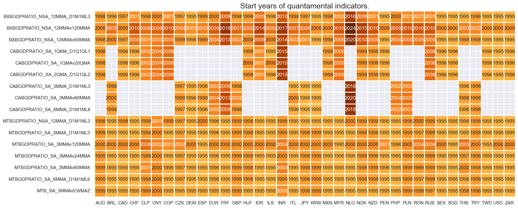
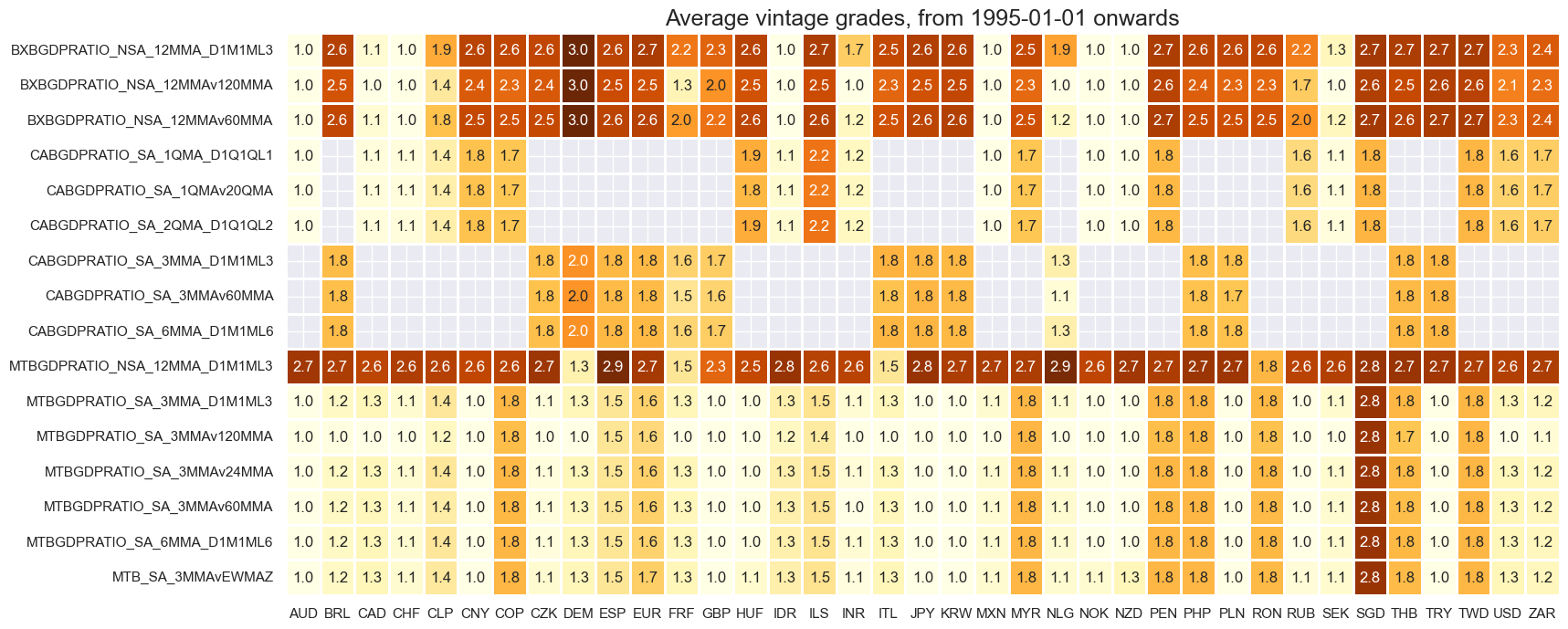
Vintage grades are mixed, with developed markets on average recording better grades than EM countries. The higher grades of seasonally-adjusted series reflect the sequential seasonal adjustment that allows deriving a good proxy of real-time data even from non-original vintages.

plot = msp.heatmap_grades(
    df,
    xcats=xcatx,
    cids=cidx,
    start=start_date,
    size=(18, 8),
    title=f"Average vintage grades, from {start_date} onwards",
)

mtbs = [
    "MTBGDPRATIO_NSA_12MMA_D1M1ML3",
    "MTBGDPRATIO_SA_3MMA_D1M1ML3",
    "MTB_SA_3MMAvEWMAZ",
]
msp.view_ranges(
    df,
    xcats=mtbs,
    cids=cids_exp,
    val="eop_lag",
    title="End of observation period lags (ranges of time elapsed since end of observation period in days)",
    start="2000-01-01",
    kind="box",
    size=(16, 4),
)
msp.view_ranges(
    df,
    xcats=mtbs,
    cids=cids_exp,
    val="mop_lag",
    title="Median of observation period lags (ranges of time elapsed since middle of observation period in days)",
    start="2000-01-01",
    kind="box",
    size=(16, 4),
)

cabs = [
    "CABGDPRATIO_SA_3MMA_D1M1ML3",
    "CABGDPRATIO_SA_6MMA_D1M1ML6",
    "CABGDPRATIO_SA_3MMAv60MMA",
    "CABGDPRATIO_SA_1QMA_D1Q1QL1",
    "CABGDPRATIO_SA_2QMA_D1Q1QL2",
    "CABGDPRATIO_SA_1QMAv20QMA",
]
msp.view_ranges(
    df,
    xcats=cabs,
    cids=cids_exp,
    val="eop_lag",
    title="End of observation period lags (ranges of time elapsed since end of observation period in days)",
    start="2000-01-01",
    kind="box",
    size=(16, 4),
)
msp.view_ranges(
    df,
    xcats=cabs,
    cids=cids_exp,
    val="mop_lag",
    title="Median of observation period lags (ranges of time elapsed since middle of observation period in days)",
    start="2000-01-01",
    kind="box",
    size=(16, 4),
)

xbbs = [
    "BXBGDPRATIO_NSA_12MMA_D1M1ML3",
    "BXBGDPRATIO_NSA_12MMAv60MMA",
    "BXBGDPRATIO_NSA_12MMAv120MMA",
]
msp.view_ranges(
    df,
    xcats=xbbs,
    cids=cids_exp,
    val="eop_lag",
    title="End of observation period lags (ranges of time elapsed since end of observation period in days)",
    start="2000-01-01",
    kind="box",
    size=(16, 4),
)
msp.view_ranges(
    df,
    xcats=xbbs,
    cids=cids_exp,
    val="mop_lag",
    title="Median of observation period lags (ranges of time elapsed since middle of observation period in days)",
    start="2000-01-01",
    kind="box",
    size=(16, 4),
)

For the purpose of the below presentation, we have renamed quarterly-frequency indicators to approximate monthly equivalents in order to have a full panel of similar measures across most countries. The two series’ are not identical but are close substitutes.

# Renaming extended categories for ease of subsequent analysis
rename_dict = {
    "CABGDPRATIO_SA_1QMA_D1Q1QL1": "CABGDPRATIO_SA_3MMA_D1M1ML3",
    "CABGDPRATIO_SA_2QMA_D1Q1QL2": "CABGDPRATIO_SA_6MMA_D1M1ML6",
    "CABGDPRATIO_SA_1QMAv20QMA": "CABGDPRATIO_SA_3MMAv60MMA",
}
dfx = df.copy()
dfx["xcat"] = df["xcat"].map(lambda x: rename_dict.get(x, x))

History

Medium-term trade balance trends

The variability of short-term trends has varied significantly across countries. Small open economies and nations with substantial commodity exports have generally seen larger fluctuations in their trade balance-to-GDP ratios. In contrast, the U.S. and the euro area have experienced the smallest standard deviations.

xcatx = ["MTBGDPRATIO_NSA_12MMA_D1M1ML3"]
cidx = cids_exp

msp.view_ranges(
    dfx,
    xcats=xcatx,
    cids=cidx,
    sort_cids_by="std",
    start=start_date,
    kind="box",
    size=(16, 8),
    title="Boxplots of medium-term trade balance trends since 1995",
    xcat_labels=["Change in 1-year moving average over preceding 3 months"],
)

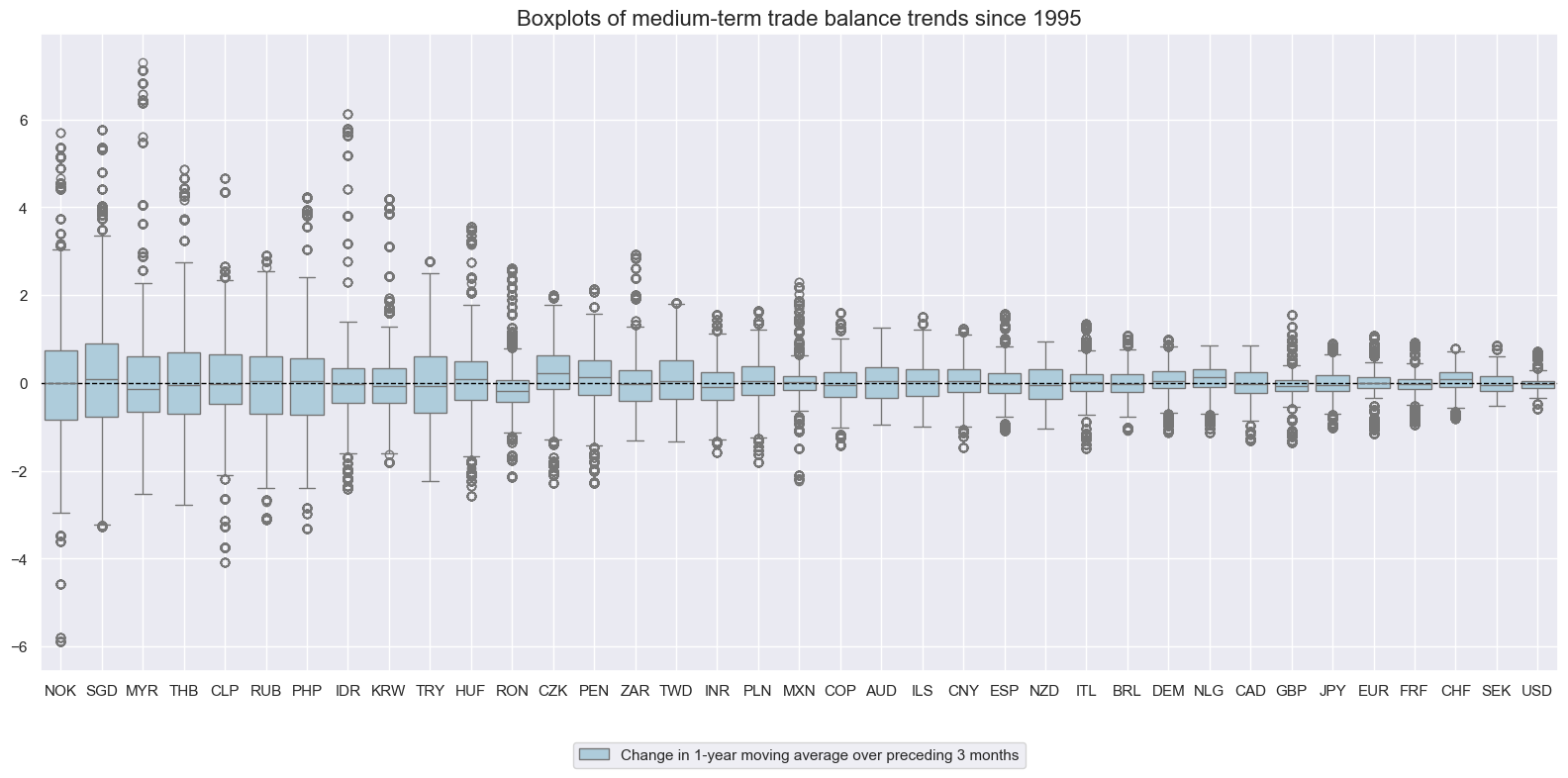
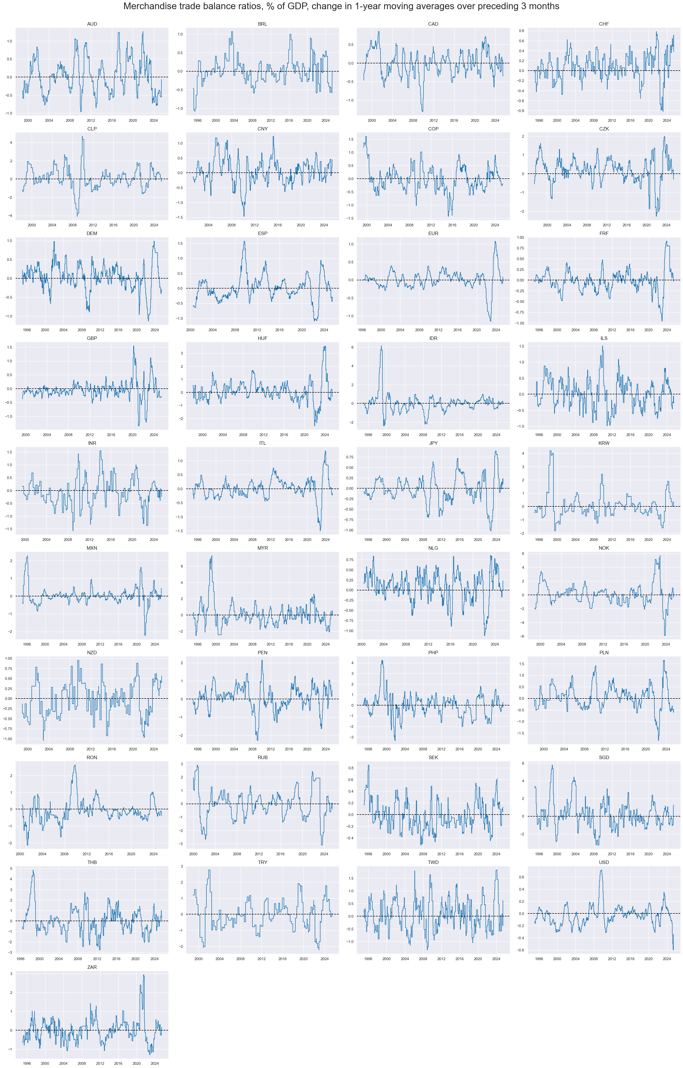
Medium-term trade balance trends have often come in cycles of 1-2 years. Large fluctuations in trade balance ratios have occurred in the wake of economic or financial turmoil.

xcatx = ["MTBGDPRATIO_NSA_12MMA_D1M1ML3"]
cidx = cids_exp

msp.view_timelines(
    dfx,
    xcats=xcatx,
    cids=cidx,
    start=start_date,
    title="Merchandise trade balance ratios, % of GDP, change in 1-year moving averages over preceding 3 months",
    title_fontsize=27,
    legend_fontsize=17,
    ncol=4,
    same_y=False,
    size=(16, 8),
    all_xticks=True,
)

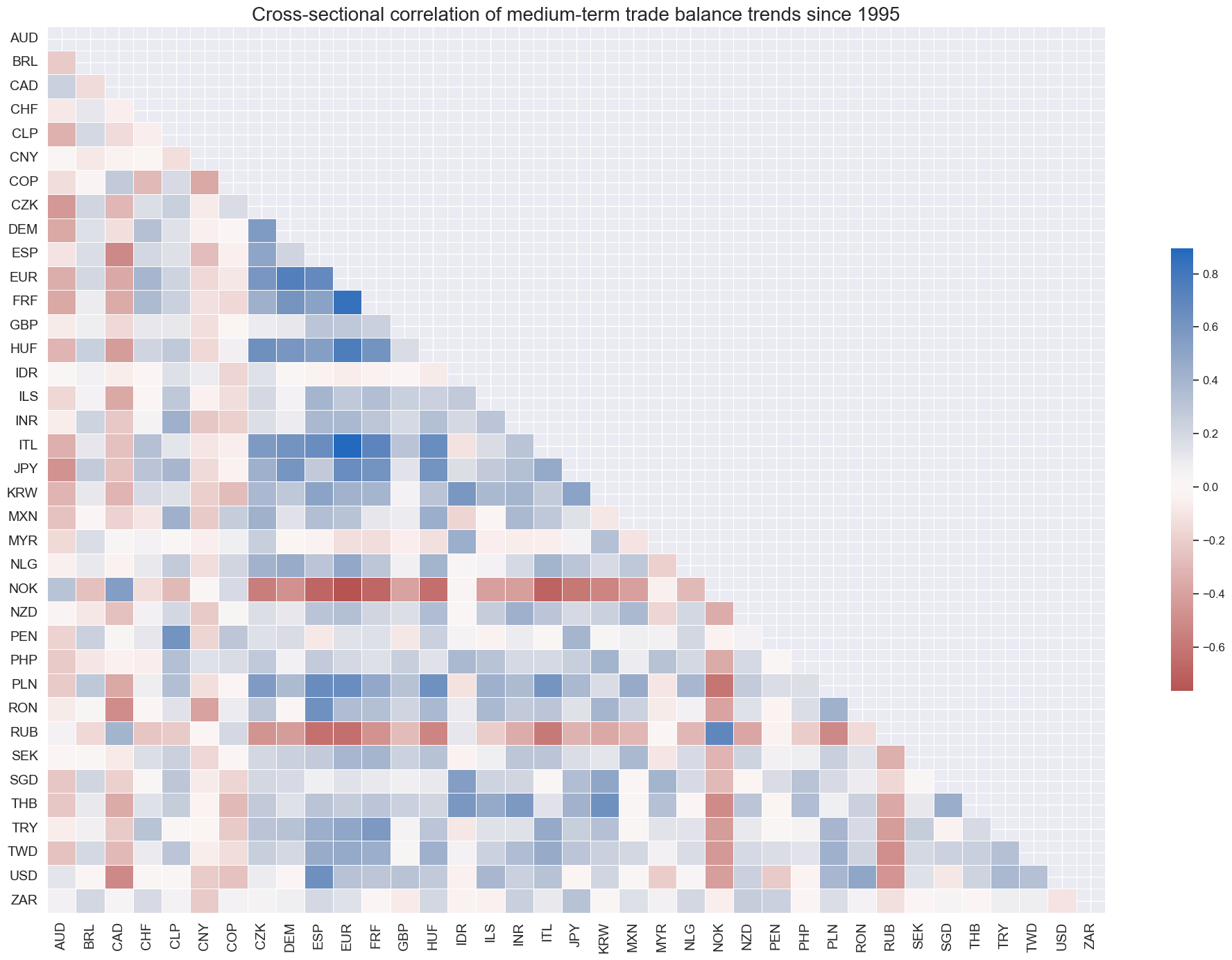
Correlations have been very diverse. Trade balance changes have been a differentiating macro factor across currency areas, with correlations plausibly depending on export-import structure and financial system features.

msp.correl_matrix(
    dfx,
    xcats="MTBGDPRATIO_NSA_12MMA_D1M1ML3",
    cids=cids_exp,
    size=(20, 14),
    start=start_date,
    title="Cross-sectional correlation of medium-term trade balance trends since 1995",
)

Short-term trade balance trends

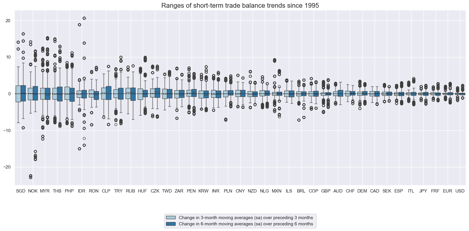
As in the case of medium-term trends, smaller countries tend to post larger short-term trade balance changes relative to GDP, since the effect of actual changes in international trade have a greater scale relative to the economy.

xcatx = ["MTBGDPRATIO_SA_3MMA_D1M1ML3", "MTBGDPRATIO_SA_6MMA_D1M1ML6"]
cidx = cids_exp

msp.view_ranges(
    dfx,
    xcats=xcatx,
    cids=cidx,
    sort_cids_by="std",
    start=start_date,
    title="Ranges of short-term trade balance trends since 1995",
    xcat_labels=[
        "Change in 3-month moving averages (sa) over preceding 3 months ",
        "Change in 6-month moving averages (sa) over preceding 6 months",
    ],
    kind="box",
    size=(16, 8),
)

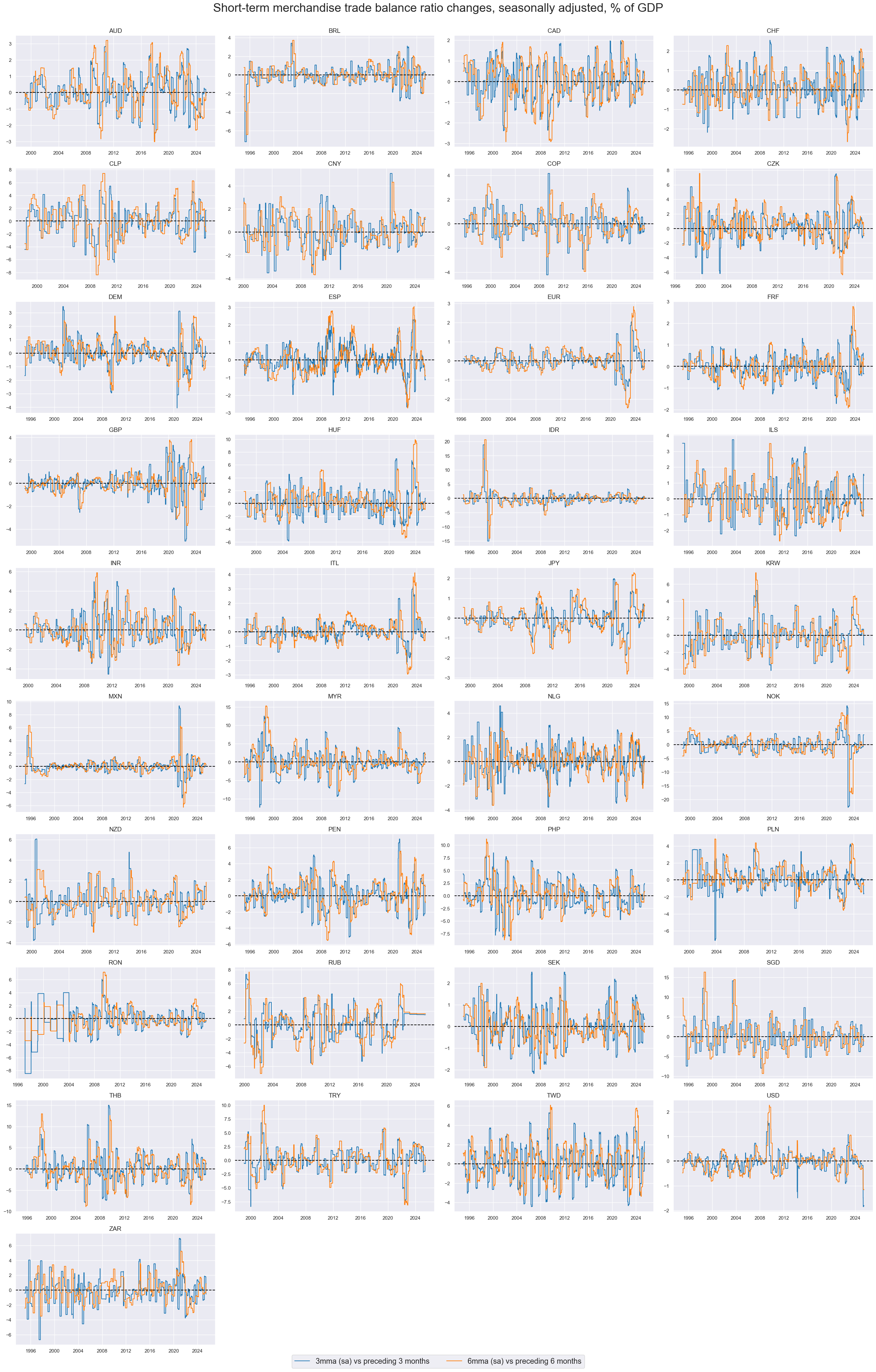
The 3-month changes in trade-balances with shorter lookback still display reveal cycles but add ample short-term volatility.

xcatx = ["MTBGDPRATIO_SA_3MMA_D1M1ML3", "MTBGDPRATIO_SA_6MMA_D1M1ML6"]
cidx = cids_exp

msp.view_timelines(
    dfx,
    xcats=xcatx,
    cids=cidx,
    start=start_date,
    title="Short-term merchandise trade balance ratio changes, seasonally adjusted, % of GDP",
    title_fontsize=27,
    legend_fontsize=17,
    xcat_labels=[
        "3mma (sa) vs preceding 3 months ",
        "6mma (sa) vs preceding 6 months",
    ],
    ncol=4,
    same_y=False,
    size=(16, 8),
    all_xticks=True,
)

Short-term current account balance trends

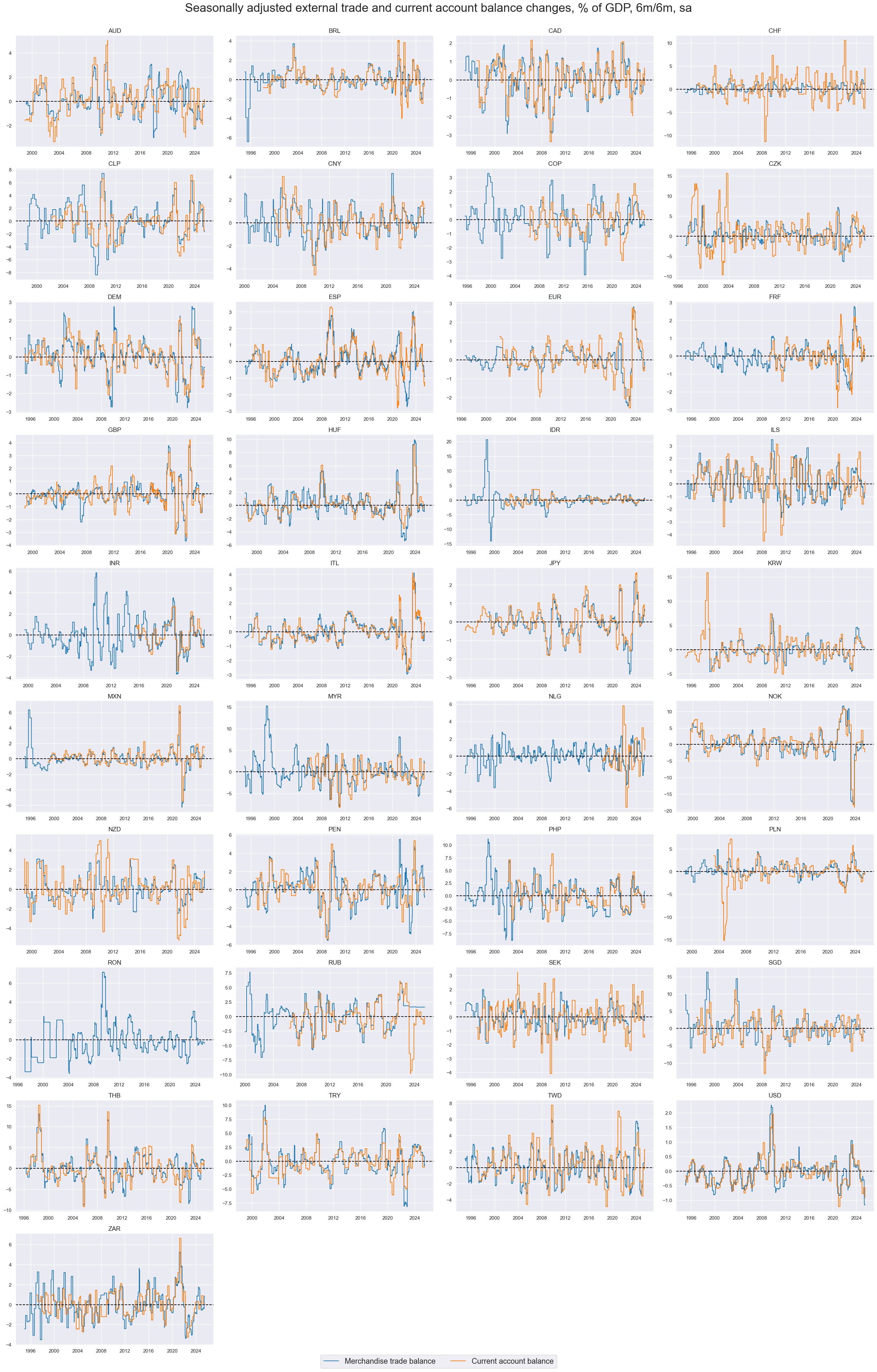
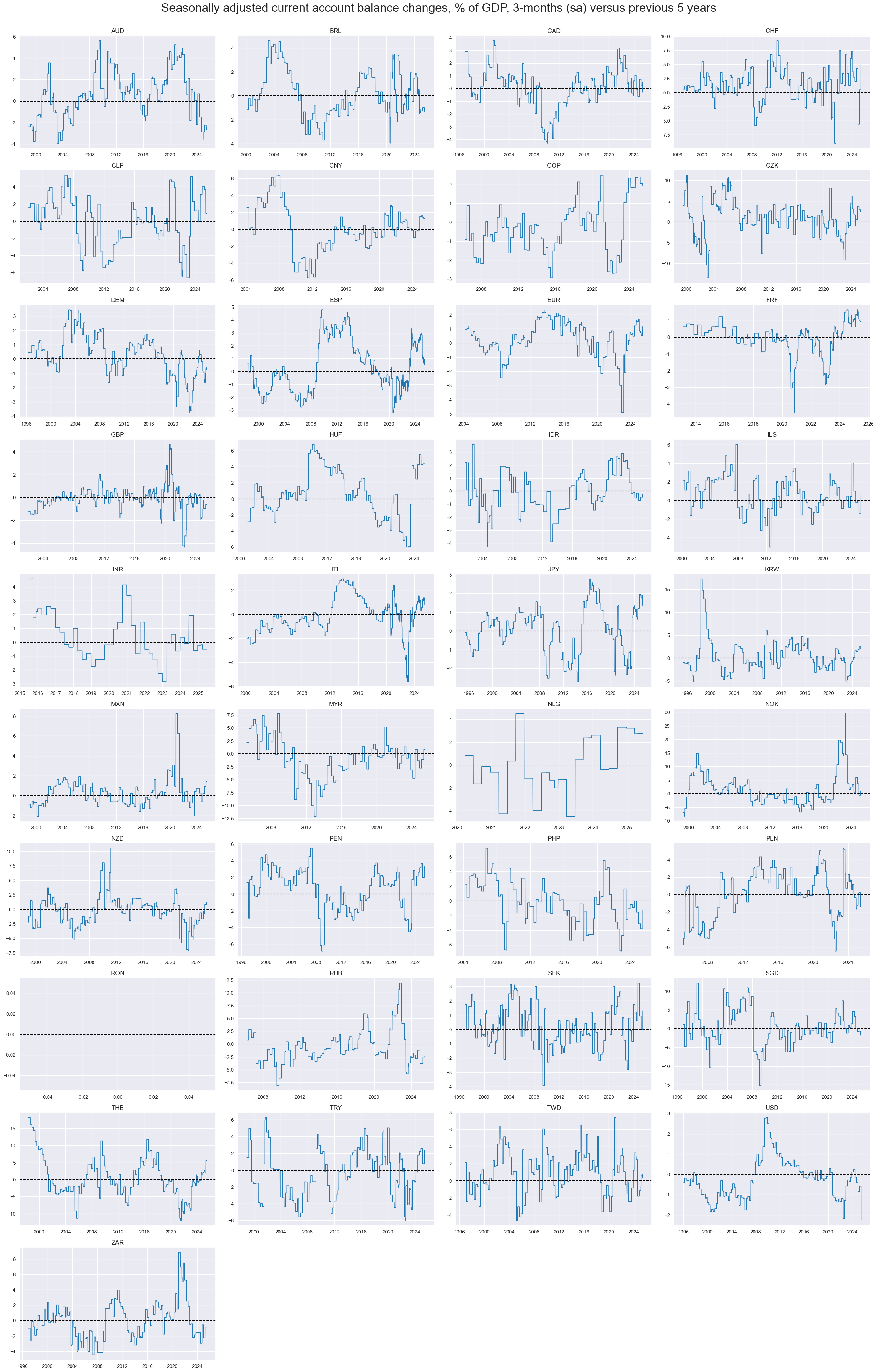
Trade balance dynamics and current account balance dynamics are naturally correlated, since the fromer is a component of the latter. However, they can have very different patterns at times. Differences can also be large for countries with a sizeable share of non-goods external trade, such as Switzerland. Information states of current account series have often shorter history than trade balance dynamics.

xcatx = ["MTBGDPRATIO_SA_6MMA_D1M1ML6", "CABGDPRATIO_SA_6MMA_D1M1ML6"]
cidx = cids_exp

msp.view_timelines(
    dfx,
    xcats=xcatx,
    cids=cids_exp,
    start=start_date,
    title="Seasonally adjusted external trade and current account balance changes, % of GDP, 6m/6m, sa",
    title_fontsize=27,
    legend_fontsize=17,
    xcat_labels=[
        "Merchandise trade balance",
        "Current account balance",
    ],
    ncol=4,
    same_y=False,
    size=(12, 7),
    all_xticks=True,
)

Longer-term trade and current account trends

Tredns versus 2-10 year moving average display only long-term developments. For most currency areas, 1-4 cycles have been observed since the beginning of the century. This means that the effect of these trends are typically best analyzed in a panel format, combining the experience of many countries.

xcatx = [
    "MTBGDPRATIO_SA_3MMAv24MMA",
    "MTBGDPRATIO_SA_3MMAv60MMA",
    "MTBGDPRATIO_SA_3MMAv120MMA",
]
msp.view_timelines(
    dfx,
    xcats=xcatx,
    cids=cidx,
    start=start_date,
    title="Longer term merchandise trade balance ratios, seasonally adjusted, % of GDP",
    title_fontsize=27,
    legend_fontsize=17,
    xcat_labels=[
        "Latest 3mma vs past 2yma",
        "Latest 3mma vs past 5yma",
        "Latest 3mma vs past 10yma",
    ],
    ncol=4,
    same_y=False,
    size=(12, 7),
    all_xticks=True,
)

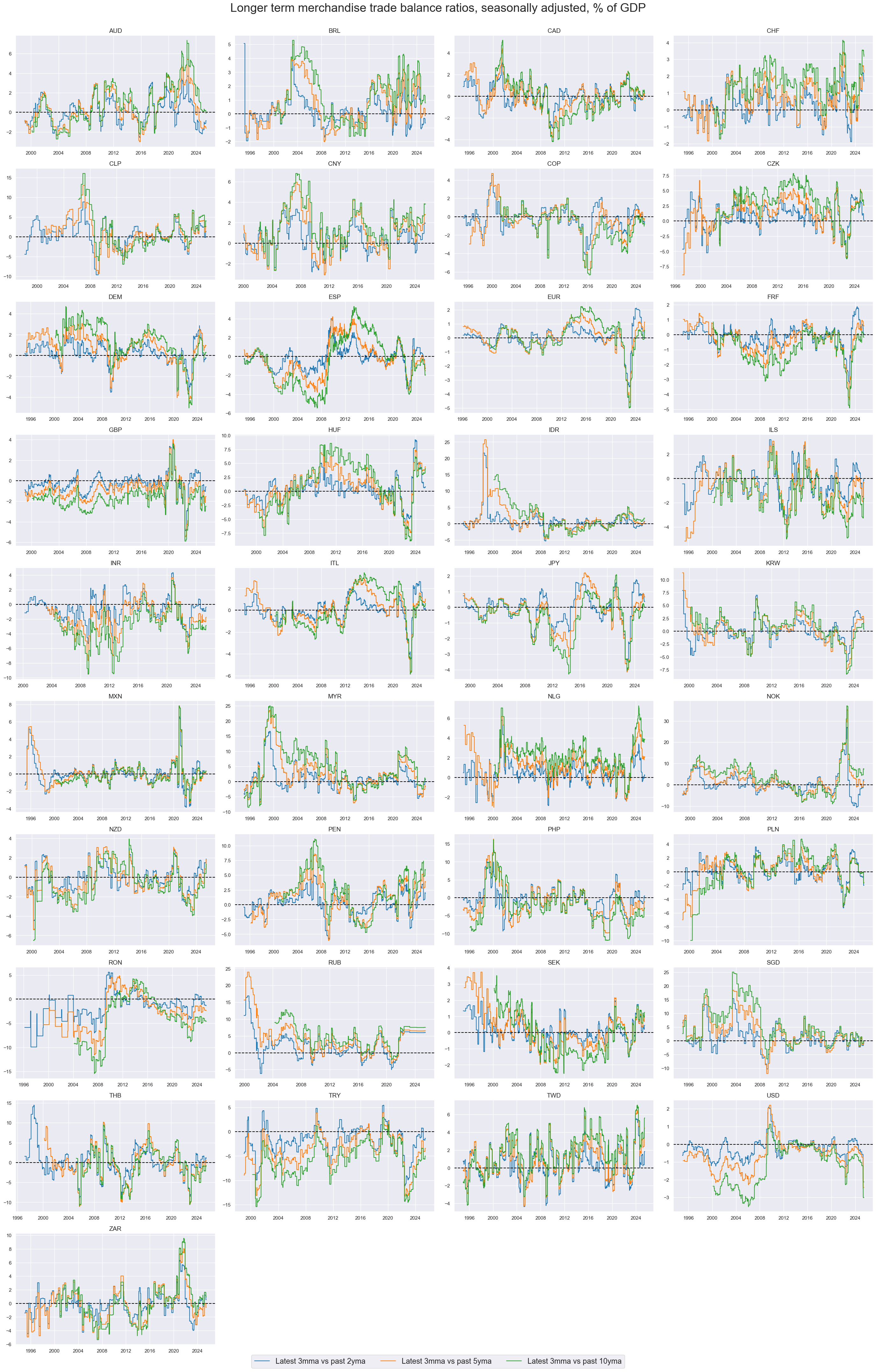
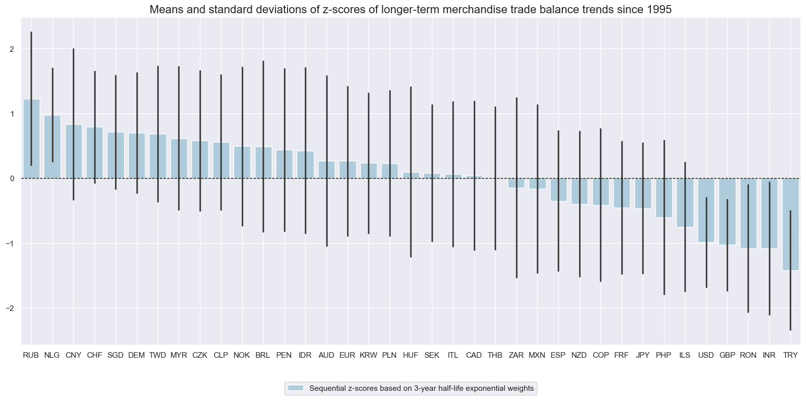
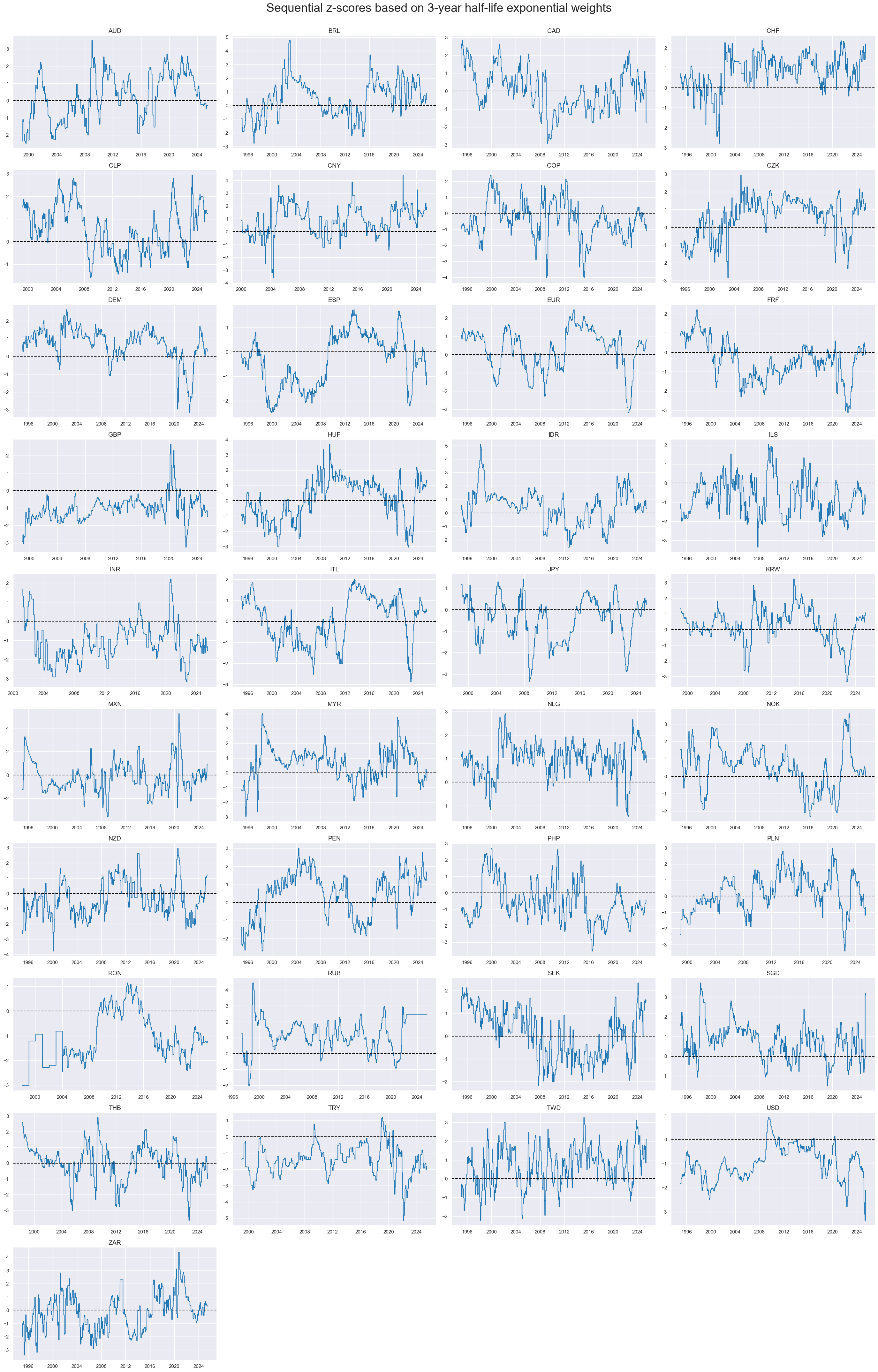
The z-score trends reveal strong long-term directional biases across countries. As trading signals they would give rise to seriously long-term positions. This reflects the use of long 3-years half-lives that are applied to the mean calculation.

xcatx = ["MTB_SA_3MMAvEWMAZ"]
cidx = cids_exp

msp.view_ranges(
    dfx,
    xcats=xcatx,
    cids=cidx,
    sort_cids_by="mean",
    start=start_date,
    title="Means and standard deviations of z-scores of longer-term merchandise trade balance trends since 1995",
    xcat_labels=["Sequential z-scores based on 3-year half-life exponential weights"],
    kind="bar",
    size=(16, 8),
)

xcatx = ["MTB_SA_3MMAvEWMAZ"]
cidx = cids_exp

msp.view_timelines(
    dfx,
    xcats=xcatx,
    cids=cidx,
    start=start_date,
    title="Sequential z-scores based on 3-year half-life exponential weights",
    title_fontsize=27,
    legend_fontsize=17,
    ncol=4,
    same_y=False,
    size=(12, 7),
    all_xticks=True,
)

xcatx = ["CABGDPRATIO_SA_3MMAv60MMA"]
cidx = cids_exp

msp.view_timelines(
    dfx,
    xcats=xcatx,
    cids=cidx,
    start=start_date,
    title="Seasonally adjusted current account balance changes, % of GDP, 3-months (sa) versus previous 5 years",
    title_fontsize=27,
    legend_fontsize=17,
    ncol=4,
    same_y=False,
    size=(12, 7),
    all_xticks=True,
)

Medium-term basic external balance trends

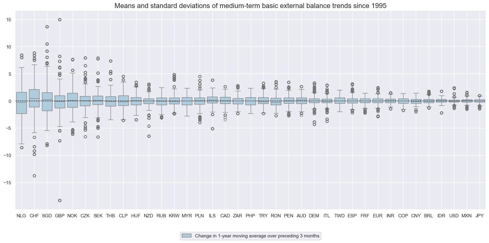
Basic external balances have posted much larger swings than trade balances, due to the variability of net FDI flows. The volatility of net FDI flows has been only partly tamed by use of trimmed (moving) means, which discard lowest and highest observations.

xcatx = ["BXBGDPRATIO_NSA_12MMA_D1M1ML3"]
cidx = cids_exp

msp.view_ranges(
    dfx,
    xcats=xcatx,
    cids=cidx,
    sort_cids_by="std",
    start=start_date,
    title="Means and standard deviations of medium-term basic external balance trends since 1995",
    xcat_labels=["Change in 1-year moving average over preceding 3 months"],
    kind="box",
    size=(16, 8),
)

xcatx = ["BXBGDPRATIO_NSA_12MMA_D1M1ML3", "MTBGDPRATIO_NSA_12MMA_D1M1ML3"]
cidx = cids_exp

msp.view_timelines(
    dfx,
    xcats=xcatx,
    cids=cids_exp,
    start=start_date,
    title="Medium term external ratios, % of GDP, change in 1-year moving averages over preceding 3 months",
    title_fontsize=27,
    legend_fontsize=17,
    xcat_labels=[
        "Basic external balance",
        "Merchandise trade balance",
    ],
    ncol=4,
    same_y=False,
    size=(12, 7),
    all_xticks=True,
)

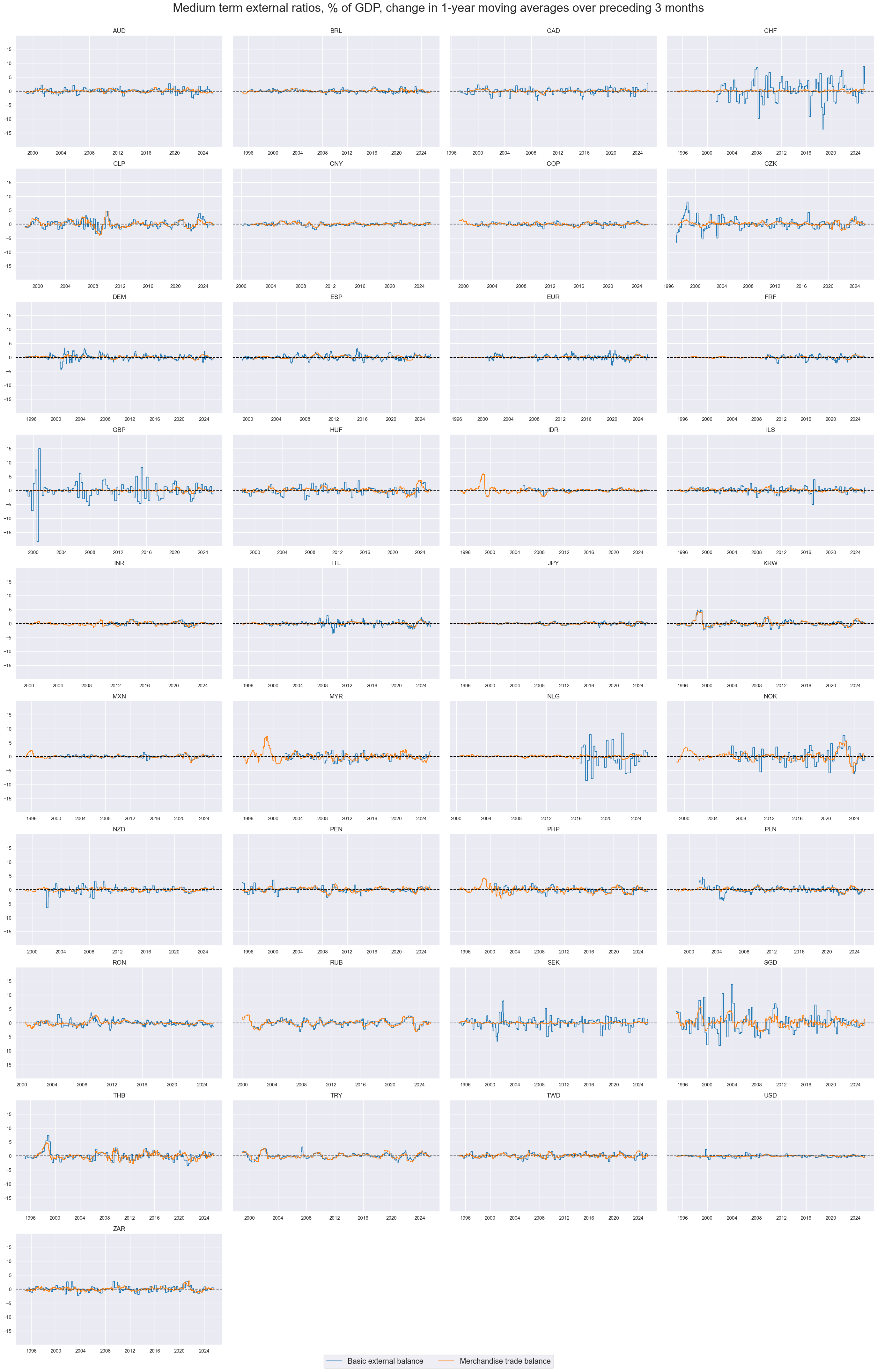
In some developed countries, such as Sweden, Norway, Switzerland and the UK, the basic external balance changes have been dominated by services, factor income and net FDI flows. Thus, the basic external balance trends bear little resemblance to the merchandise trade balance trends.

xcatx = ["BXBGDPRATIO_NSA_12MMA_D1M1ML3", "MTBGDPRATIO_NSA_12MMA_D1M1ML3"]
cidx = ["CHF", "SEK", "GBP"]
msp.view_timelines(
    dfx,
    xcats=xcatx,
    cids=cidx,
    start=start_date,
    title="Medium term external ratios, % of GDP, change in 1-year moving averages over preceding 3 months",
    title_fontsize=27,
    legend_fontsize=17,
    same_y=False,
    xcat_labels=["Basic external balance trend", "Merchandise trade balance"],
)

Longer-term basic external balance trends

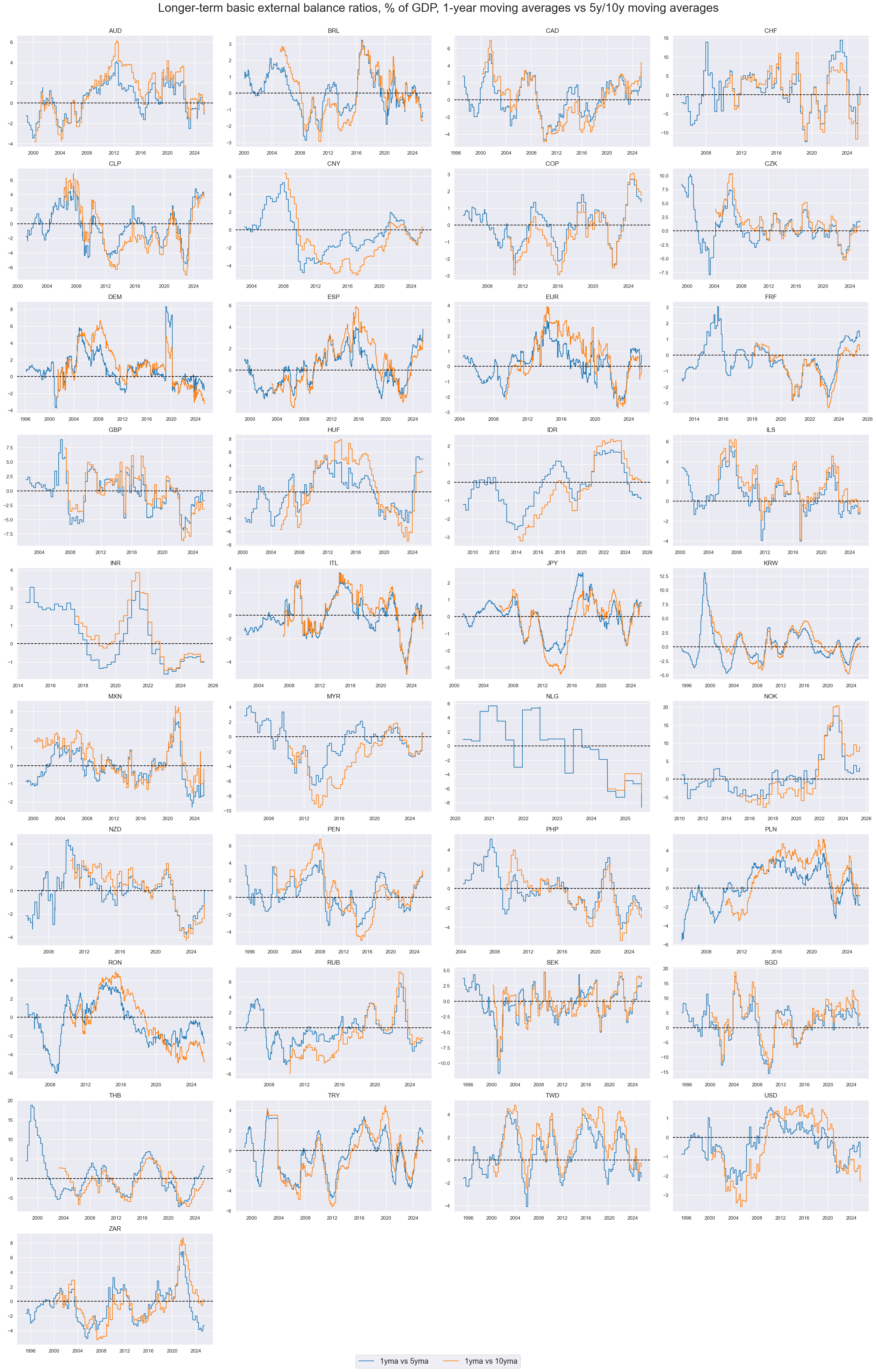
The 12-month ratios versus 5-10 year averages naturally only capture very long cycles. These may be particularly useful indicators of the underlying structural changes in the competitiveness of countries.

xcatx = [
    "BXBGDPRATIO_NSA_12MMAv60MMA",
    "BXBGDPRATIO_NSA_12MMAv120MMA",
]
cidx = cids_exp

msp.view_timelines(
    dfx,
    xcats=xcatx,
    cids=cidx,
    start=start_date,
    title="Longer-term basic external balance ratios, % of GDP, 1-year moving averages vs 5y/10y moving averages",
    title_fontsize=27,
    legend_fontsize=17,
    xcat_labels=[
        "1yma vs 5yma",
        "1yma vs 10yma",
    ],
    ncol=4,
    same_y=False,
    size=(12, 7),
    all_xticks=True,
)

Importance

Research links

On exchange rate flexibility and external balance adjustments

“For 181 countries…we find a significant and empirically robust relationship between exchange rate flexibility and the speed of external adjustment. Our results are supported by several ‘natural experiments’ of exogenous changes in bilateral exchange rate regimes.” Ghosh, Qureshi, and Tsangarides, 2014

On external ratios and economic growth

“…deterioration of trade balance has a negative impact on economic growth or vice versa. The results of multivariate regression analysis (model I) confirm statistically significant negative trade balance impact on economic growth.” Trade Balance Effects on Economic Growth: Evidence from European Union Countries

“…generally trade balance deterioration reduces average economic growth and from linear relationship evaluation we can state that it does not matter whether it starts from trade deficit or surplus result…” Trade Balance Effects on Economic Growth: Evidence from European Union Countries

“…large and persistent current account deficits driven by government borrowing are likely to be troublesome down the road if not matched by productivity gains or productive investment in tradable sectors.” Maurico Obstfeld

“… Excluding the US, we find that size does matter: the length of current account deficit spells is negatively related to the relative size of the countries’ GDP. “ J Aizenman and Y Sun

On external ratios and FX

“…a simple error-correction model that uses terms-of-trade variables seems to have an empirically significant ability to forecast exchange rate changes out-of-sample… [in Canada]” Robert A Amano

“The sign and size of the current account balance points to the expected long-run real exchange rate adjustment, but portfolio positions determine the vulnerability to sharp exchange rate fluctuations.” Maurico Obstfeld

“The external strength score is a plausible predictor of volatility-targeted FX forward returns. These are returns of FX forwards of a long in the local currency versus the base currency in percent of risk capital on a position that is scaled to a 10% (annualized) volatility target.” Macrosynergy

“…currency areas with large external deficits, highly negative international investment positions, or poor economic performance pose – all other things equal – a risk of sudden bouts of depreciation.” Macrosynergy

“…For simple growth differentials, the statistical probability of positive correlation with subsequent returns has been near 100% with a quite stable relationship across time. … balanced growth differentials that emphasize equally the performance of output and external balances are theoretically a sounder predictor. Macrosynergy

“(a) throughout the sample period the vast majority of countries have run current account deficits… (b) Large current account deficits have not had a significant degree of persistence through time. Only a few countries have run persistently large deficits. (c) The degree of persistence of large surpluses has been higher… (e) Major reversals in current account deficits have tended to be persistent through time, and strongly associated to “sudden stops” of capital inflows. (f) There is a high probability that reversals lead to an exchange rate crisis; the evidence also indicates that countries that try to face reversals by running down reserves significantly usually do not succeed.” Sebastian Edwards

“…Canada’s experience has indicated that rising debt levels can lead to higher real interest rates as risk premia increase. Moreover, a real exchange rate depreciation will eventually be required to restore external balance. This is most easily achieved in a flexible exchange rate environment.” James Powell, Bank of Canada

On external ratios and equity returns

“…our results seem to hint towards the notion that the current account has information for predictability of the equity premium when the market is not doing well because in those states investors are looking for more macroeconomic information, while when the markets are booming there is more herding into the markets and less interest in searching out for relevant marco-economic information on behalf of the market agents.” Rangan Gupta, Anandamayee Majumdar & Mark E. Wohar

On external ratios and real estate

“We find a robust and strong positive association between current account deficits and the appreciation of the real estate prices…Controlling for lagged GDP/capita growth, inflation, financial depth, institution, urban population growth and the real interest rate; a one standard deviation increase of the lagged current account deficits is associated with an appreciation of the real estate prices by 10%. “ Joshua Aizenman and Yothin Jinjarak

Empirical clues

Identifying and isolating periods characterized by official exchange rate targets, illiquidity, or convertibility-related distortions in FX markets is crucial for testing any FX-based hypothesis. These periods can significantly influence the behavior and dynamics of currency markets, and neglecting to account for them can result in inaccurate or misleading conclusions. Therefore, we compile a blacklist of such periods for all cross-sections to ensure accurate analysis.

# Blacklist periods of FX targeting or illiquidity

dfb = dfx[dfx["xcat"].isin(["FXTARGETED_NSA", "FXUNTRADABLE_NSA"])].loc[
    :, ["cid", "xcat", "real_date", "value"]
]
dfba = (
    dfb.groupby(["cid", "real_date"])
    .aggregate(value=pd.NamedAgg(column="value", aggfunc="max"))
    .reset_index()
)
dfba["xcat"] = "FXBLACK"
fxblack = msp.make_blacklist(
    dfba, "FXBLACK"
)  # dictionary of periods of FX targeting or illiquidity

External ratios and FX forward returns

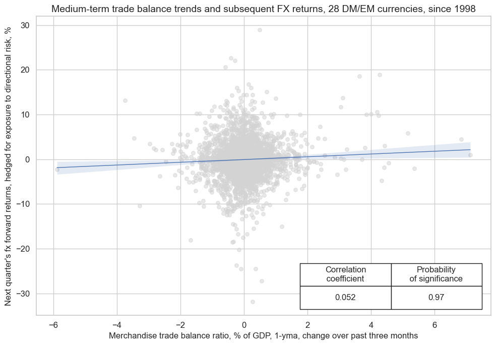
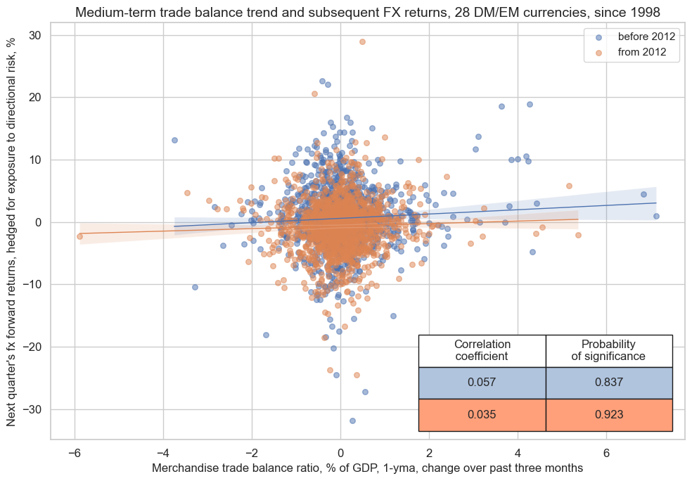
Panel regression has shown a signficant positive relation between end-of-month information states of medium term external ratios and subsequent weekly, monthly and quarterly hedged FX returns . The relation is quite seasonal, however, and requires episodes of balance of payments crises and recoveries to manifest.

Hedged return here means that the FX forward position is combined with a position in a global directional risk basket. The global directional risk basket contains equal volatility-weights in equity index futures, CDS indices and FX forwards. See also the notes on the ‘directional risk basket returns’ category DRBXR_NSA here .

cr = msp.CategoryRelations(
    dfx,
    xcats=["MTBGDPRATIO_NSA_12MMA_D1M1ML3", "FXXRHvGDRB_NSA"],
    cids=cids_fx,
    freq="q",
    lag=1,
    xcat_aggs=["last", "sum"],
    start="1998-01-01",
    blacklist=fxblack,
)

cr.reg_scatter(
    title="Medium-term trade balance trends and subsequent FX returns, 28 DM/EM currencies, since 1998",
    xlab="Merchandise trade balance ratio, % of GDP, 1-yma, change over past three months",
    ylab="Next quarter's fx forward returns, hedged for exposure to directional risk, %",
    prob_est="map",
    coef_box="lower right",
    size=(10, 7),
)

cr.reg_scatter(
    title="Medium-term trade balance trend and subsequent FX returns, 28 DM/EM currencies, since 1998",
    xlab="Merchandise trade balance ratio, % of GDP, 1-yma, change over past three months",
    ylab="Next quarter's fx forward returns, hedged for exposure to directional risk, %",
    prob_est="map",
    coef_box="lower right",
    separator=2012,
    size=(10, 7),
)

External ratio changes and interest rate swap returns

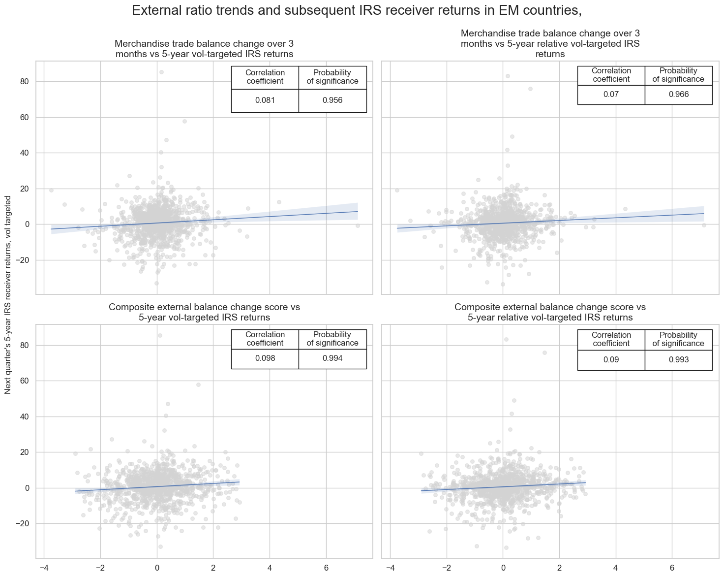
Plausibly, there should a a positive relationships between external ratio trends and the local currency IRS returns, both directional and relative to USD IRS returns. That is because improving external balances increase the chances of unsterilized FX interventions with increasing local liquidity while they reduce the risk of overvaluation and sudden stops in capital flows. The latter is particularly important for emerging markets economies that rely on foreign funding.

To simplify the analysis we calculate a composite of different external balance dynamics, using with euqal weights [i] 3-month changes in 12-month basic external balances ratios, [ii] 3-month changes in 12-month merchandise trade balances ratio, and [iii] short-term changes in monthly seasonally-adjusted merchanidse trade balances (3m/3m and 6m/6m).

# Calculate a composite score for external balance dynamics

xcatx = [
    "BXBGDPRATIO_NSA_12MMA_D1M1ML3",
    "MTBGDPRATIO_NSA_12MMA_D1M1ML3",
    "MTBGDPRATIO_SA_3MMA_D1M1ML3",
    "MTBGDPRATIO_SA_6MMA_D1M1ML6",
]  # shorter term dynamics
cidx = cids_exp


dfa = pd.DataFrame(columns=dfx.columns)


for xc in xcatx:

    dfaa = msp.make_zn_scores(
        dfx,
        xcat=xc,
        cids=cidx,
        sequential=True,
        min_obs=522,  # oos scaling after 2 years of panel data
        est_freq="m",
        neutral="zero",
        pan_weight=1,
        thresh=3,
        postfix="_ZN",

    )

    dfa = msm.update_df(dfa, dfaa)

dfx = msm.update_df(dfx, dfa)


dix = {
    "BXBGDPRATIO_NSA_12MMA_D1M1ML3_ZN": 1 / 3,
    "MTBGDPRATIO_NSA_12MMA_D1M1ML3_ZN": 1 / 3,
    "MTBGDPRATIO_SA_3MMA_D1M1ML3_ZN": 1 / 6,
    "MTBGDPRATIO_SA_6MMA_D1M1ML6_ZN": 1 / 6,
}


dfa = msp.linear_composite(
    dfx,
    xcats=list(dix.keys()),
    weights=list(dix.values()),
    cids=cidx,
    complete_xcats=False,
    new_xcat="XBDYNZ_AVG",
)

dfx = msm.update_df(dfx, dfa)

# Calculate relative returns versus the U.S.


targs = ["DU05YXR_VT10"]


dfa = msp.make_relative_value(
    dfx, xcats=targs, cids=cids, basket=["USD"], postfix="vUSD"
)


dfx = msm.update_df(dfx, dfa)

There is pervasive evidence of a positive relation between external balances changes and subsequent local currency IRS returns in emerging markets since 1998. The relationship has been signficant for both relative and directional returns, as well as for simple trade balance changes and the composite external balance change score.

Since is important, since currrency areas with strong relative and growth and high real carry often display deteriorating external balances. The empirical relevance of the latter advices to include external balance dynamics in carry trade signals.

# Define the target categories
targ_dict = {
    "DU05YXR_VT10": "5-year vol-targeted IRS returns",
    "DU05YXR_VT10vUSD": "5-year relative vol-targeted IRS returns",
}

# Define easy-to-read labels for the signals
xlab_dict = {
    "MTBGDPRATIO_NSA_12MMA_D1M1ML3": "Merchandise trade balance change over 3 months",
    "XBDYNZ_AVG": "Composite external balance change score",
}

cids_emexp = list(
    set(cids_em) - set(["BRL", "PEN", "PHP", "RON", "INR", "SGD", "TWD"])
)  # all emerging markets that trade IRS

# Initialize the dictionary to store CategoryRelations instances
cr = {}

# Loop through the signals and target categories
for sig in xlab_dict.keys():
    for targ in targ_dict.keys():
        cr[f"cr_{sig}_{targ}"] = msp.CategoryRelations(
            dfx,
            xcats=[sig, targ],
            cids=cids_emexp,
            freq="Q",
            lag=1,
            xcat_aggs=["last", "sum"],
            start="1998-01-01",
            blacklist=fxblack,
        )

# Combine all CategoryRelations instances for plotting
all_cr_instances = [
    cr[f"cr_{sig}_{targ}"] for sig in xlab_dict.keys() for targ in targ_dict.keys()
]

# Define all labels for the subplot titles
all_labels = [
    f"{sig} vs {targ}" for sig in xlab_dict.values() for targ in targ_dict.values()
]

# Plotting the results
msv.multiple_reg_scatter(
    cat_rels=all_cr_instances,
    title="External ratio trends and subsequent IRS receiver returns in EM countries, ",
    ylab="Next quarter's 5-year IRS receiver returns, vol targeted",
    ncol=2,
    nrow=len(all_labels) // 2,  # Adjust the number of rows based on the number of plots
    figsize=(15, 12),
    prob_est="map",
    coef_box="upper right",
    subplot_titles=all_labels,
)

Long-term trends and relative sovereign CDS returns.

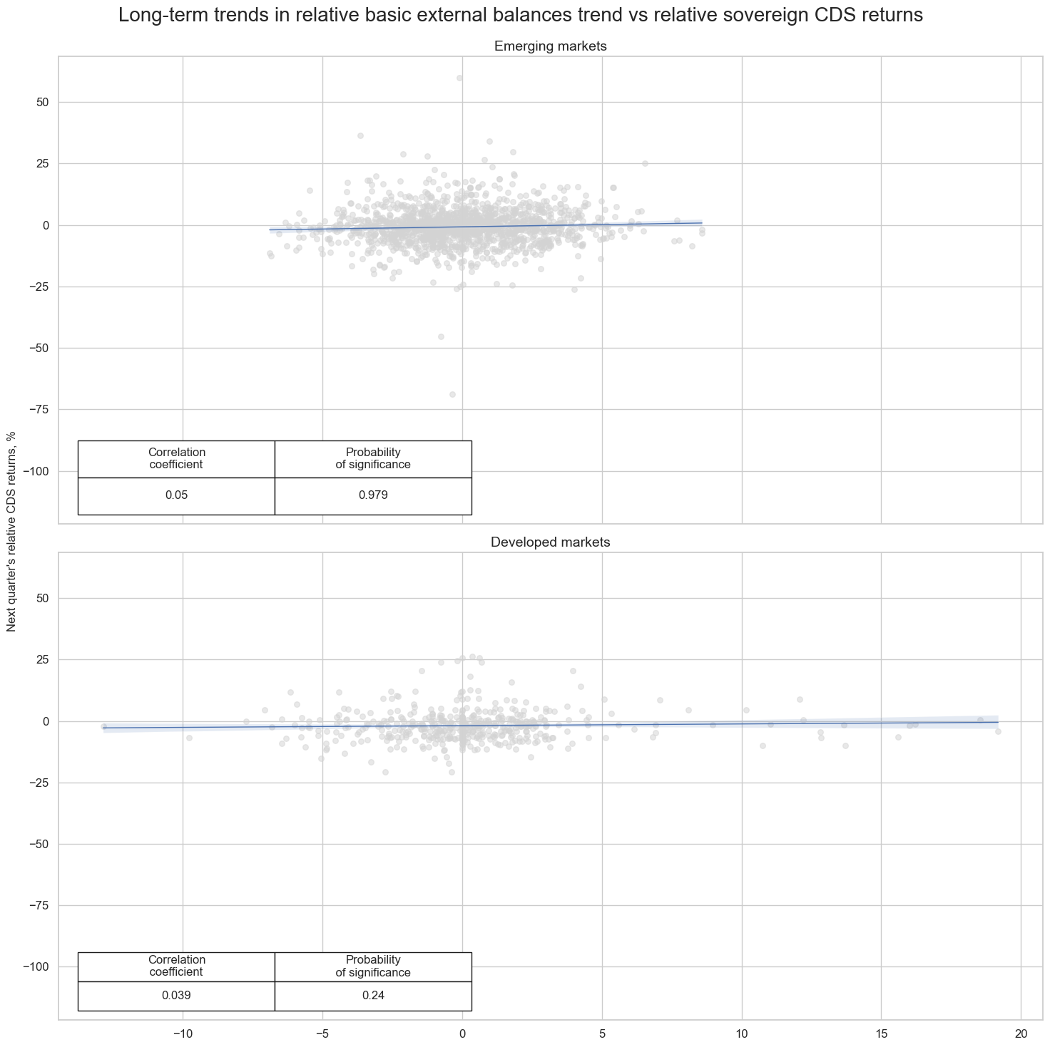
In this section, we explore the relationships between long-term external ratios and the returns on sovereign credit default swaps (CDS) relative to U.S. high yield CDS index.

The hypothesis is that countries with imporving external balances are less likely to incur sudden stops of capital flows and resulting funding problems than those with deteriorating external balances. Empirically, we find that the relationship between long-term external balance trends and relative sovereign CDS returns is positive. It is signficant only for emerging markets, however, and not for developed markets.

# Define replacements for corporate bond identifiers
replacements = {
    "EHY": ("_EHY", "EUR"),  # High yield EUR corporate bonds
    "EIG": ("_EIG", "EUR"),  # Investment grade EUR corporate bonds
    "UHY": ("_UHY", "USD"),  # High yield USD corporate bonds
    "UIG": ("_UIG", "USD"),  # Investment grade USD corporate bonds
}

# Apply the replacements to the dataframe
for cid, (suffix, new_cid) in replacements.items():
    condition = dfx["cid"] == cid
    dfx.loc[condition, "xcat"] = dfx.loc[condition, "xcat"] + suffix
    dfx.loc[condition, "cid"] = new_cid

# Define external ratio trend categories
xcatx = ["BXBGDPRATIO_NSA_12MMAv60MMA"]

# Create relative value data for the specified categories
dfa = msp.make_relative_value(
    dfx, xcats=xcatx, cids=cids, basket=["USD"], postfix="vUSD"
)

# Update the original dataframe with the new data
dfx = msm.update_df(dfx, dfa)

# Define calculations for relative CDS returns
calcs = [
    "CDS05YXR_VT10vUHY = ( CDS05YXR_VT10 - iUSD_CRXR_VT10_UHY )",
]

# Apply the calculations to the dataframe
dfa = msp.panel_calculator(dfx, calcs, cids=cids)
dfx = msm.update_df(dfx, dfa)

cids_emexp = list(
    set(cids_em) - set(["INR", "SGD", "TWD"])
)  # all available emerging markets cross-sections
cids_dmexp = list(
    set(cids_dmca) - set(["CAD", "EUR"])
)  # all available developed markets cross-sections

cr_cds_em = {}
cr_cds_dm = {}


# Create CategoryRelations for cr_cds_em
cr_cds_em = msp.CategoryRelations(
    dfx,
    xcats=["BXBGDPRATIO_NSA_12MMAv60MMAvUSD", "CDS05YXR_VT10vUHY"],
    cids=cids_emexp,
    freq="Q",
    blacklist=fxblack,
    lag=1,
    xcat_aggs=["last", "sum"],
    start=start_date,
)

# Create CategoryRelations for cr_cds_dm
cr_cds_dm = msp.CategoryRelations(
    dfx,
    xcats=["BXBGDPRATIO_NSA_12MMAv60MMAvUSD", "CDS05YXR_VT10vUHY"],
    cids=cids_dmexp,
    freq="Q",
    blacklist=fxblack,
    lag=1,
    xcat_aggs=["last", "sum"],
    start=start_date,
)

msv.multiple_reg_scatter(
    cat_rels=[cr_cds_em] + [cr_cds_dm],
    title="Long-term trends in relative basic external balances trend vs relative sovereign CDS returns",
    ylab="Next quarter's relative CDS returns, %",
    ncol=1,
    nrow=2,
    figsize=(15, 15),
    prob_est="map",
    coef_box="lower left",
    subplot_titles=["Emerging markets", "Developed markets"],
)

Appendices

Appendix 1: Seasonal adjustment procedure

We deploy the state-of-the-art US Census X-13 algorithm to handle seasonality in economic series. There are two characteristics of the model worth noting in connection to the point-in-time estimation JPMaQS is delivering:

1. The underlying econometric model is a seasonal ARIMA model leveraging a two-sided filter. As both the earliest and latest observations are included in the historical seasonal component estimation, JPMaQS forces the model (and seasonal component) to being re-estimated for each release date’s time-series. This ensures that only information available at a given point-in-time is used, avoiding leakage of future information.

2. The algorithm has an embedded endogenous model specification using an Akaike Information Criteria, ensuring the parameters are dynamically chosen using only information available at each point-in-time.

For our seasonally adjustment of the Merchandise Trade Balances , we sequentially apply the multiplicative method of the U.S. Census X-13 algorithm to the levels of imports and exports respectively for each of their vintages. We then subtract the imports from the exports to get the seasonally adjusted merchandise trade balances, and take ratios to nominal GDP at the end. This contrast with the Current Account Balances , were we first take the ratio to GDP to deal deal with non-stationarity in the data, and then apply the additive X-13 method to these ratios for each release date. As current account balances can be both in surplus and deficit, we cannot use the multiplicative method to deal with the non-stationarity of the data.

Appendix 2: Notes on OECD data integration

Some indicators in this notebook are constructed using vintages provided by the OECD’s Revision Analysis Dataset in addition to national sources series’. The integration of the OECD datasets follows the following rules:

1. The following priority order is applied for combining vintages. First, JPMaQS uses seasonally and calendar adjusted original vintages from national sources. Beyond that JPMaQS uses OECD vintages.

2. OECD vintages inform on the month of release but not the exact date. Actual release dates for these vintages are estimated based on release days of subsequent vintages.

3. Inconsistencies, data errors and missing values in the OECD vintages have been corrected for JPMaQS.

OECD data is seasonally adjusted and denominated in native currency. No such consistency is found in national sources. Often figures are stated in a foreign denomination (EUR or USD) and no seasonal adjustment has been applied. To integrate these two data sources we first currency convert national sources into their native currency and then apply seasonal adjustment.

Appendix 3: Currency symbols

The word ‘cross-section’ refers to currencies, currency areas or economic areas. In alphabetical order, these are AUD (Australian dollar), BRL (Brazilian real), CAD (Canadian dollar), CHF (Swiss franc), CLP (Chilean peso), CNY (Chinese yuan renminbi), COP (Colombian peso), CZK (Czech Republic koruna), DEM (German mark), ESP (Spanish peseta), EUR (Euro), FRF (French franc), GBP (British pound), HKD (Hong Kong dollar), HUF (Hungarian forint), IDR (Indonesian rupiah), ITL (Italian lira), JPY (Japanese yen), KRW (Korean won), MXN (Mexican peso), MYR (Malaysian ringgit), NLG (Dutch guilder), NOK (Norwegian krone), NZD (New Zealand dollar), PEN (Peruvian sol), PHP (Philippine peso), PLN (Polish zloty), RON (Romanian leu), RUB (Russian ruble), SEK (Swedish krona), SGD (Singaporean dollar), THB (Thai baht), TRY (Turkish lira), TWD (Taiwanese dollar), USD (U.S. dollar), ZAR (South African rand).