FX forward returns

The category group contains daily FX forward returns of tradeable, floating, and convertible currencies, for tenors of 1 month to 1 year. By default, returns are calculated against their respective dominant cross, which will be the USD, EUR or an equally weighted basket of both. We also provide subcategories comprising returns against the USD only. All calculations assume monthly roll at the end of the month back to full 1-month maturity, regardless of the forward tenor.

We calculate the FX forwards returns of going long the base currency , including the roll-down intra-monthly, in two steps. Firstly, we calculate the annualised carry as:

(8) \[\begin{equation} CRY_{t} = \left(\frac{S_{t}}{F_{t}}\right)^{1/h} - 1 \end{equation}\]

Where \(S_{t}\) is the FX spot price, \(F_{t}\) is the forward contract of tenor \(h\) (i.e. 1m forward: \(h=1/12\) ).

In the second stage, we use the no-arbitrage condition from Covered Interest Parity to calculate the forward price for each day (off the roll date), adjusting for days remaining in the month ( day-count-fraction : \({dcf}_{t}\) ):

(9) \[\begin{equation} {Fb}_{t} = S_{t} (1 + {CRY}_{t})^{-{dcf_{t}}} \end{equation}\]

Using the above, excess returns are then easily calculated as follows:

(10) \[\begin{equation} {XR}_{t} = \begin{cases} \frac{Fb_{t}}{Fb_{t-1}} -1 & \forall\textrm{intra monthly}\\ \frac{Fb_{t}}{F_{t-1}} -1 & \forall\textrm{after a roll-date}. \end{cases} \end{equation}\]

The FX spot and forward prices are from the JP Morgan trading desks, with Asian, European, and USDCAD taken at London close. Latin American FX crosses (USDBRL, USDCLP, USDCOP, USDMXN, and USDPEN) are end-of-day mark of each country’s trading desk.

FX forward return in % of notional

Ticker : FXXR_NSA / FXXRUSD_NSA

Label : FX forward return, % of notional: dominant cross / against USD.

Definition : 1-month FX forward return, % of notional of the contract, assuming roll back to full 1-month maturity at the end of the month: long against natural benchmark currencies / long against USD.

Notes :

• The default returns are calculated for a contract that is long the local currency of the cross section against its dominant traded benchmark.

• The benchmark for Switzerland, Czechoslovakia, Hungary, Norway, Poland, Romania and Sweden is the euro, whilst Great Britain, Turkey and Russia use an equally weighted basket of dollars and euros. All other cross-sections use the dollar as a benchmark.

• USD-compared returns are added separately for convenience should one wish to work with a pure USD-based panel.

• For the following currencies, returns are at least partly based on non-deliverable contracts: Brazil, Chile, China, Indonesia, India, South Korea, Malaysia and Taiwan. Chile is deliverable as of 2021.

• For some currencies, the returns include periods of low liquidity and FX targeting. If one wishes to ‘blacklist’ such periods, one should use the non-tradability and FX-target dummmies, which have category ticker codes FXUNTRADABLE_NSA and FXTARGETED_NSA . Malaysia, as an example, is frequently blacklisted between 1999 and the end of 2007.

Vol-targeted FX forward return

Ticker : FXXR_VT10 / FXXRUSD_VT10

Label : FX forward return for 10% vol target: dominant cross / against USD.

Definition : 1-month FX forward return, % of risk capital on position scaled to 10% (annualized) volatility target, assuming roll back to full 1-month maturity at the end of the month: long against natural benchmark currencies / long against USD.

Notes :

• Positions are scaled to a 10% volatility target based on historic standard deviation for an exponential moving average with a half-life of 11 days. Positions are rebalanced at the end of each month. Moreover, a maximum leverage ratio of 5 (of implied notional to cash position) is imposed.

• See the important related notes on “FX forward return in % of notional” above.

Hedged FX forward return

Ticker : FXXRHvGDRB_NSA

Label : Return on FX forward, hedged against market direction risk.

Definition : Return on 1-month FX forward position that has been hedged against directional risk through a position in a global directional risk basket, % of forward notional, rolled at the end of the month.

Notes :

• The global directional risk basket contains equal volatility-weights in equity index futures, CDS indices and FX forwards. See also the notes on the ‘directional risk basket returns’ category DRBXR_NSA here .

• Hedge ratios are calculated based on historical “beta”, i.e. weighted least-squares regression coefficients of past forward returns with respect to global directional risk basket returns. The estimate uses two regressions. One is based on monthly returns with an exponentially-weighted lookback of 24-months half-life. The other is based on daily returns with an exponentially-weighted lookback of 63 trading days. The usage of the two lookbacks seeks to strike a balance between timeliness of information and structural relations.

• See the important related notes on “FX forward return in % of notional” above.

FX forward return for longer tenors in % of notional

Ticker : FX03MXR_NSA / FX06MXR_NSA / FX09MXR_NSA / FX01YXR_NSA

Label : FX forward return, % of notional, vs dominant cross: 3m tenor / 6m tenor / 9m tenor / 1y tenor.

Definition : FX forward return, % of notional of the contract, assuming roll back to full equivalent maturity at the end of the month, against natural benchmark currency: 3-month forward / 6-month forward / 9-month forward / 1-year forward.

Notes :

• The default returns are calculated for a contract that is long the local currency of the cross section against its dominant traded benchmark.

• The benchmark for Switzerland, Czechoslovakia, Hungary, Norway, Poland, Romania and Sweden is the euro, whilst Great Britain, Turkey and Russia use an equally weighted basket of dollars and euros. All other cross-sections use the dollar as a benchmark.

• For the following currencies, returns are at least partly based on non-deliverable contracts: Brazil, Chile, China, Indonesia, India, South Korea, Malaysia and Taiwan. Chile is deliverable as of 2021.

• For some currencies, the returns include periods of low liquidity and FX targeting. If one wishes to ‘blacklist’ such periods, one should use the non-tradability and FX-target dummmies, which have category ticker codes FXUNTRADABLE_NSA and FXTARGETED_NSA . Malaysia, as an example, is frequently blacklisted between 1999 and the end of 2007.

Vol-targeted FX forward return for longer tenors

Ticker : FX03MXR_VT10 / FX06MXR_VT10 / FX09MXR_VT10 / FX01YXR_VT10

Label : FX forward return for 10% vol target, vs dominant cross: 3m tenor / 6m tenor / 9m tenor / 1y tenor.

Definition : FX forward return, % of risk capital on position scaled to 10% (annualized) volatility target, assuming roll back to full equivalent maturity at the end of the month, against natural benchmark currency: 3-month forward / 6-month forward / 9-month forward / 1-year forward.

Notes :

• Positions are scaled to a 10% volatility target based on historic standard deviation for an exponential moving average with a half-life of 11 days. Positions are rebalanced at the end of each month. Moreover, a maximum leverage ratio of 5 (of implied notional to cash position) is imposed.

• See the important related notes on “FX forward return in % of notional” above.

Imports

Only the standard Python data science packages and the specialized macrosynergy package are needed.

import os
import numpy as np
import pandas as pd
import matplotlib.pyplot as plt
import seaborn as sns
import math

import json
import yaml

import macrosynergy.management as msm
import macrosynergy.panel as msp
import macrosynergy.signal as mss
import macrosynergy.pnl as msn
import macrosynergy.visuals as msv


from macrosynergy.download import JPMaQSDownload

from timeit import default_timer as timer
from datetime import timedelta, date, datetime

import warnings

warnings.simplefilter("ignore")

The JPMaQS indicators we consider are downloaded using the J.P. Morgan Dataquery API interface within the macrosynergy package. This is done by specifying ticker strings , formed by appending an indicator category code <category> to a currency area code <cross_section> . These constitute the main part of a full quantamental indicator ticker, taking the form DB(JPMAQS,<cross_section>_<category>,<info>) , where <info> denotes the time series of information for the given cross-section and category. The following types of information are available:

• value giving the latest available values for the indicator

• eop_lag referring to days elapsed since the end of the observation period

• mop_lag referring to the number of days elapsed since the mean observation period

• grade denoting a grade of the observation, giving a metric of real time information quality.

After instantiating the JPMaQSDownload class within the macrosynergy.download module, one can use the download(tickers,start_date,metrics) method to easily download the necessary data, where tickers is an array of ticker strings, start_date is the first collection date to be considered and metrics is an array comprising the times series information to be downloaded.

# Cross-sections of interest

cids_dmca = [
    "AUD",
    "CAD",
    "CHF",
    "EUR",
    "GBP",
    "JPY",
    "NOK",
    "NZD",
    "SEK",
    "USD",
]  # DM currency areas
cids_latm = ["BRL", "COP", "CLP", "MXN", "PEN"]  # Latam countries
cids_emea = ["CZK", "HUF", "ILS", "PLN", "RON", "RUB", "TRY", "ZAR"]  # EMEA countries
cids_emas = [
    "CNY",
    # "HKD",
    "IDR",
    "INR",
    "KRW",
    "MYR",
    "PHP",
    "SGD",
    "THB",
    "TWD",
]  # EM Asia countries

cids_dm = cids_dmca
cids_em = cids_latm + cids_emea + cids_emas

cids = sorted(cids_dm + cids_em)
cids_fx = sorted(list(set(cids) - set(["USD"])))

main = [
    "FXXR_NSA",
    "FX03MXR_NSA",
    "FX06MXR_NSA",
    "FX09MXR_NSA",
    "FX01YXR_NSA",
    "FXXR_VT10",
    "FX03MXR_VT10",
    "FX06MXR_VT10",
    "FX09MXR_VT10",
    "FX01YXR_VT10",
    "FXXRHvGDRB_NSA",
    "FXXRUSD_NSA",
    "FXXRUSD_VT10",
]

econ = [
    "RGDPTECH_SA_P1M1ML12_D3M3ML3",
    "CTOT_NSA_P1M1ML12",
    "CTOT_NSA_P1M12ML1",
    "CTOT_NSA_P1W4WL1",
    "MBCSCORE_SA",
    "MBCSCORE_SA_D3M3ML3",
    "UNEMPLRATE_SA_D3M3ML3",
    "UNEMPLRATE_SA_D1Q1QL1"
]

fxcr = [
    f"FX{tenor}CRR_{adj}"
    for adj in ["NSA", "VT10"]
    for tenor in ["03M", "06M", "09M", "01Y"]
]
mark = [
    "EQXR_NSA",
    "FXXRBETAvGDRB_NSA",
    "FXTARGETED_NSA",
    "FXUNTRADABLE_NSA",
    "FXCRR_NSA",
    "FXCRR_VT10",
    "FXCRRUSD_NSA",
    "FXCRRUSD_V10",
] + fxcr  # related market categories

xcats = main + econ + mark

# Download series from J.P. Morgan DataQuery by tickers

start_date = "1990-01-01"
tickers = [cid + "_" + xcat for cid in cids for xcat in xcats]
print(f"Maximum number of tickers is {len(tickers)}")

# Retrieve credentials

client_id: str = os.getenv("DQ_CLIENT_ID")
client_secret: str = os.getenv("DQ_CLIENT_SECRET")

# Download from DataQuery

with JPMaQSDownload(client_id=client_id, client_secret=client_secret) as downloader:
    start = timer()
    assert downloader.check_connection()
    df = downloader.download(
        tickers=tickers,
        start_date=start_date,
        metrics=["value", "eop_lag", "mop_lag", "grading"],
        suppress_warning=False,
        show_progress=True,
    )
    end = timer()

dfd = df

print("Download time from DQ: " + str(timedelta(seconds=end - start)))

Maximum number of tickers is 1184
Downloading data from JPMaQS.
Timestamp UTC:  2024-11-15 12:04:36
Connection successful!

Requesting data: 100%|██████████| 237/237 [00:48<00:00,  4.86it/s]
Downloading data: 100%|██████████| 237/237 [01:07<00:00,  3.50it/s]

Some expressions are missing from the downloaded data. Check logger output for complete list.
444 out of 4736 expressions are missing. To download the catalogue of all available expressions and filter the unavailable expressions, set `get_catalogue=True` in the call to `JPMaQSDownload.download()`.
Some dates are missing from the downloaded data. 
2 out of 9102 dates are missing.
Download time from DQ: 0:02:15.851504

Availability

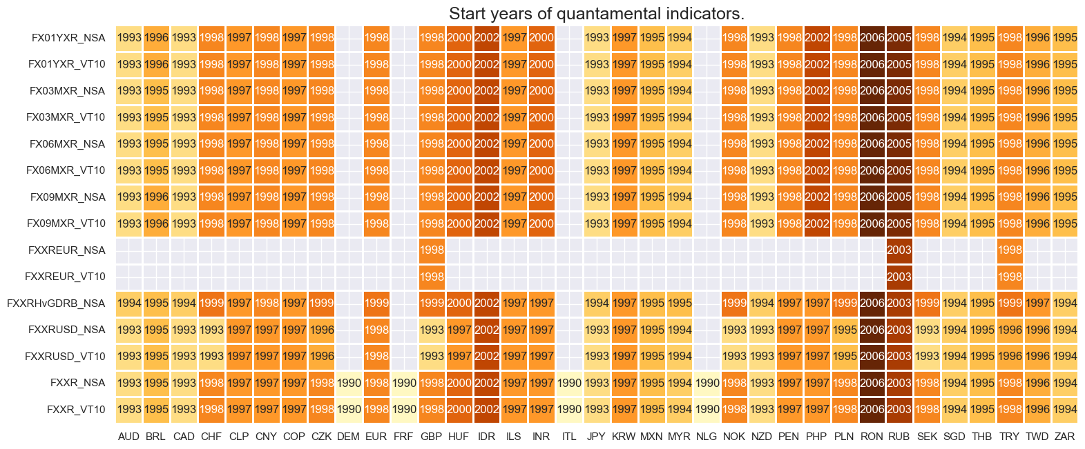
For most currencies, the return series are available back to 2000. Late starters are Romania, Russia and Indonesia, whose forward markets developed later.

For the explanation of currency symbols, which are related to currency areas or countries for which categories are available, please view Appendix 1 .

xcatx = main
cidx = cids_fx

dfx = msm.reduce_df(dfd, xcats=xcatx, cids=cidx)
dfs = msm.check_startyears(
    dfx,
)
msm.visual_paneldates(dfs, size=(18, 6))

print("Last updated:", date.today())

Last updated: 2024-11-15

xcatx = main
cidx = cids_fx

plot = msm.check_availability(
    dfd, xcats=xcatx, cids=cidx, start_size=(18, 3), start_years=False
)

History

FX forward returns in % of notional

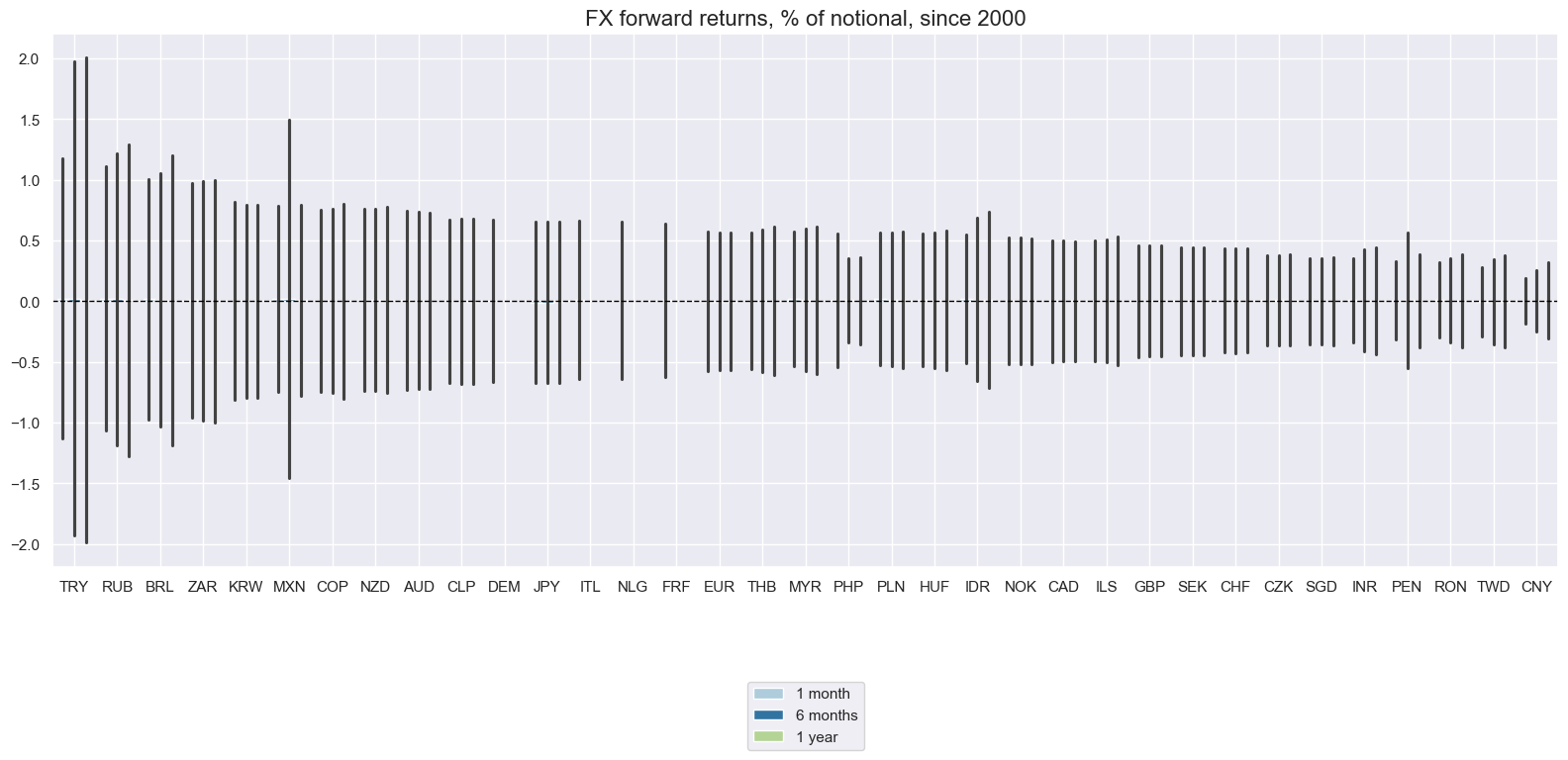
Long-term daily standard deviations of FX forward returns have displaying different orders of magnitude across countries, depending on exchange rate regimes, openness of the economies, and macroeconomic stability. Outliers have been common, with recorded daily returns of up to 40%. The Turkish lira (TRY) posted the biggest gain in December 2021 after the introduction of a local-currency deposit insurance mechanism against exchange rate depreciation and accompanying interventions.

Volatility of long-term tenors has typically been larger than for short-term tenors, with the 1-year tenor being the most volatile.

xcatx = ["FXXR_NSA", "FX06MXR_NSA", "FX01YXR_NSA"]
cidx = cids_fx

msp.view_ranges(
    dfd,
    xcats=xcatx,
    cids=cidx,
    sort_cids_by="std",
    start="2000-01-01",
    kind="bar",
    title="FX forward returns, % of notional, since 2000",
    xcat_labels=["1 month", "6 months", "1 year"],
    size=(16, 8),
)

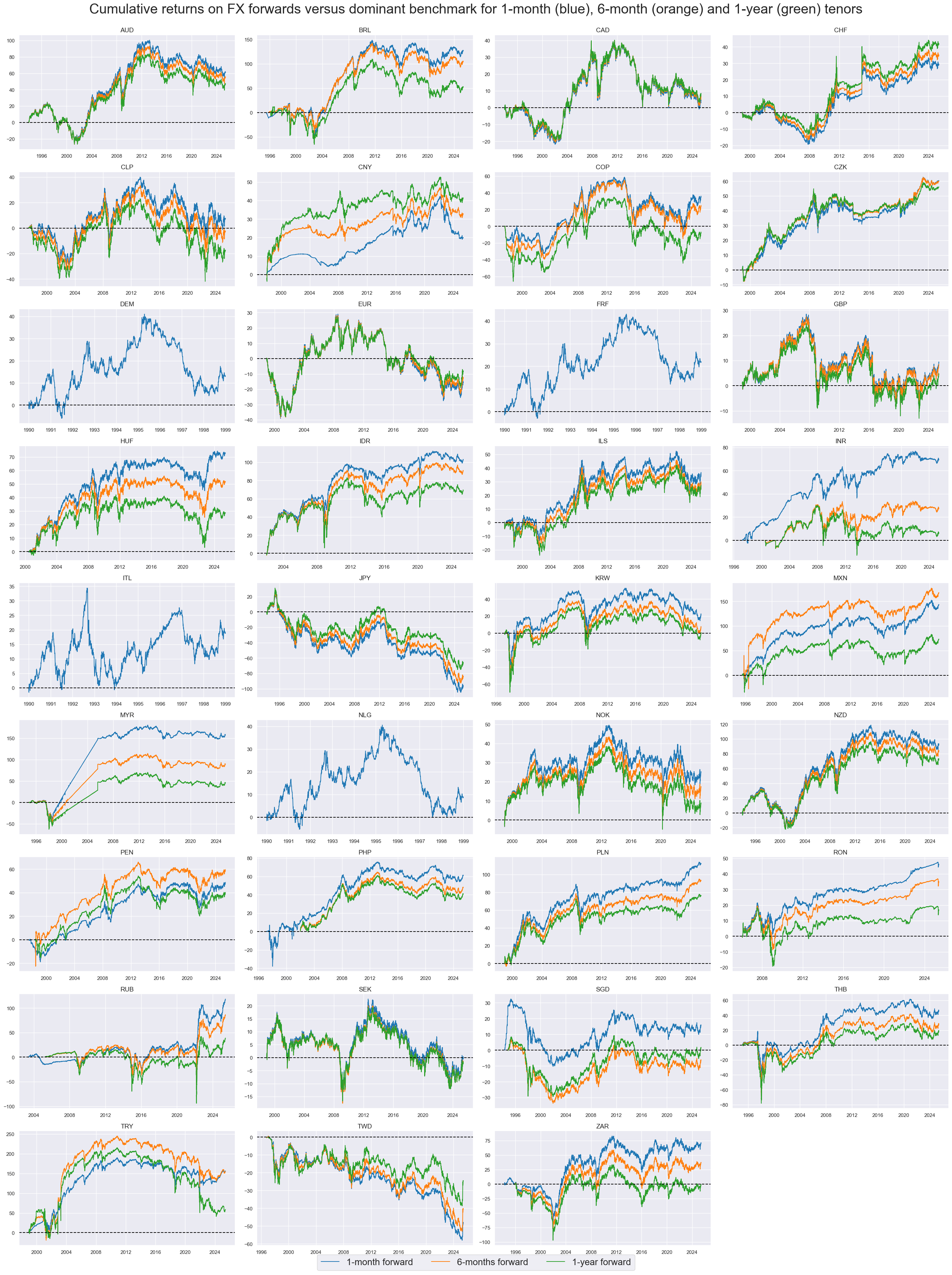
FX returns have recorded very different dynamics across currency areas, unlike equity returns and fixed-income returns. Also, lomg-term performances have been vastly different.

The below cumulative returns have not always been accessible to international investors since some EM countries imposed periods of tight capital controls. To exclude these periods, one should include the information of the “FX tradeability and flexibility” category. Particularly striking examples include the performance of the Malaysian ringgit in the early 2000s and the recorded massive positive return on the Russian ruble in the initial phase of the Ukraine invasion.

xcatx = ["FXXR_NSA", "FX06MXR_NSA", "FX01YXR_NSA"]
cidx = cids_fx 

msp.view_timelines(
    dfd,
    xcats=xcatx,
    xcat_labels=["1-month forward", "6-months forward", "1-year forward"],
    cids=cidx,
    start="2000-01-01",
    title="Cumulative returns on FX forwards versus dominant benchmark for 1-month (blue), 6-month (orange) and 1-year (green) tenors",
    title_fontsize=30,
    legend_fontsize=20,
    cumsum=True,
    ncol=4,
    same_y=False,
    size=(12, 7),
    aspect=1.7,
    all_xticks=True,
)

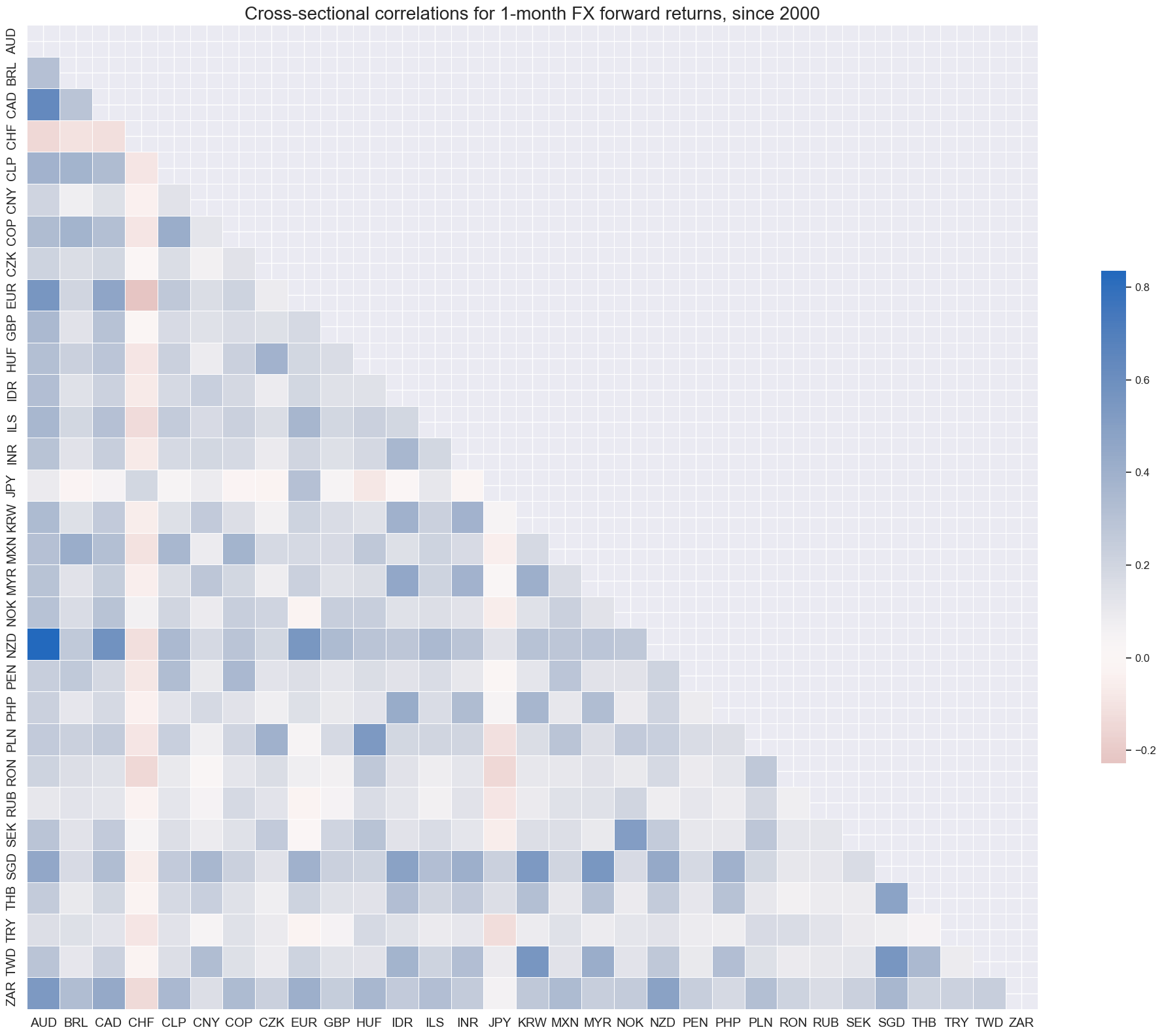
Cross-sectional correlations across forward returns have been mostly positive. This should be expected since the U.S dollar is the common benchmark for most currencies and many EM currencies have been positively correlated with global equity and credit returns. Two notable “negative correlators” have been CHF and JPY, both of which have historically served as funding currencies for positions in global and EM currencies.

xcatx = "FXXR_NSA"
cidx = cids_fx

msp.correl_matrix(
    dfd,
    xcats=xcatx,
    cids=cidx,
    title="Cross-sectional correlations for 1-month FX forward returns, since 2000",
    size=(20, 16),
)

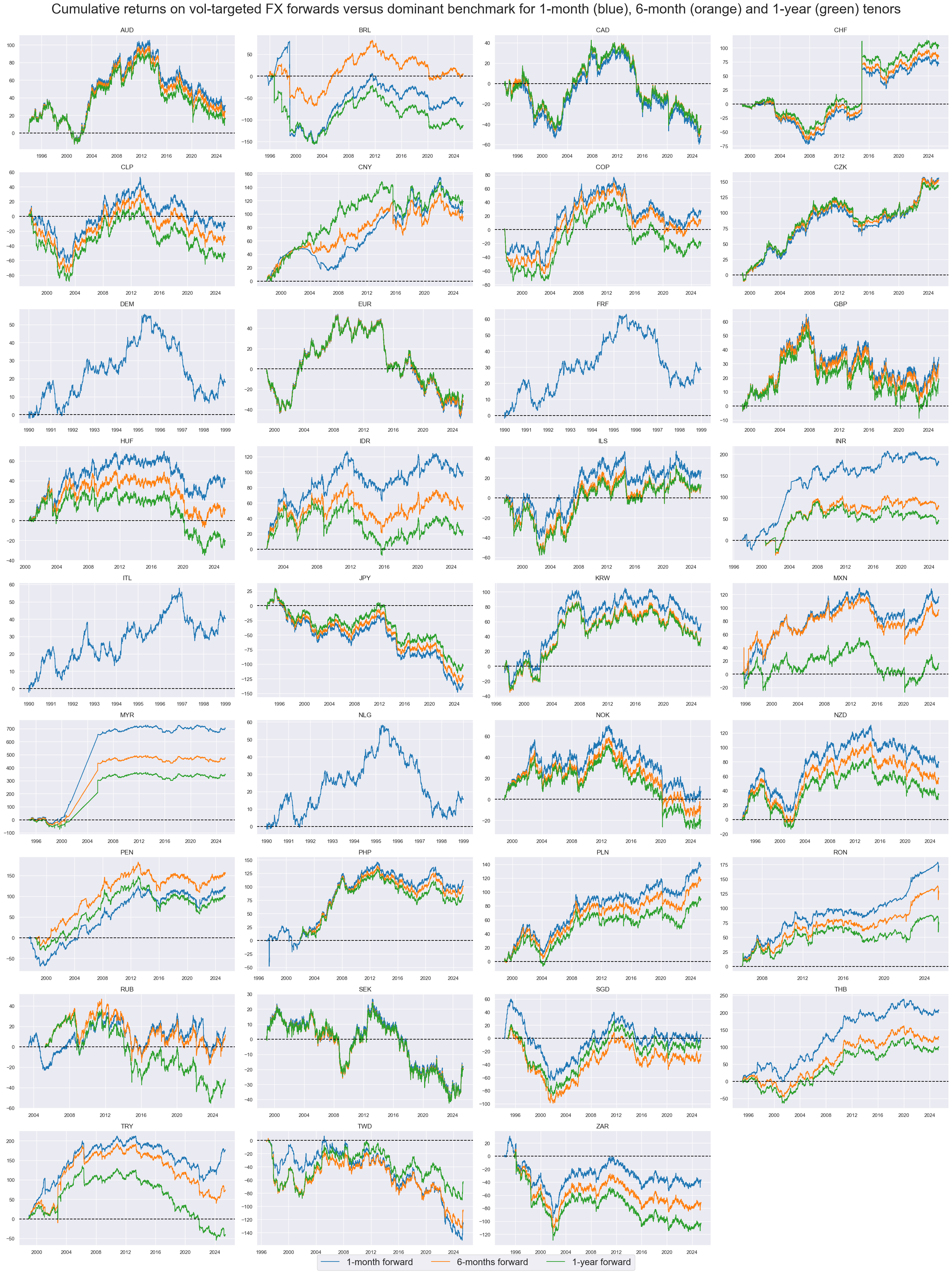
Vol-targeted FX forward returns

Long-term standard deviations are similar across volatility targeted returns. However, there have been conspicuous outliers. The proclivity to large outliers arises due the mechanical application of the volatility targeting. In periods of exchange rate targeting or pegging, they induce excessive leverage, leading to huge volatility targeted returns from the break of pegs.

xcatx = ["FXXR_VT10", "FX03MXR_VT10", "FX01YXR_VT10"]
cidx = cids_fx

msp.view_ranges(
    dfd,
    xcats=xcatx,
    cids=cidx,
    sort_cids_by="std",
    start="2000-01-01",
    kind="box",
    title="Boxplots for 10% volatility-targeted FX forward returns, since 2000",
    xcat_labels=["1 month", "3 months", "1 year"],
    size=(16, 8),
)

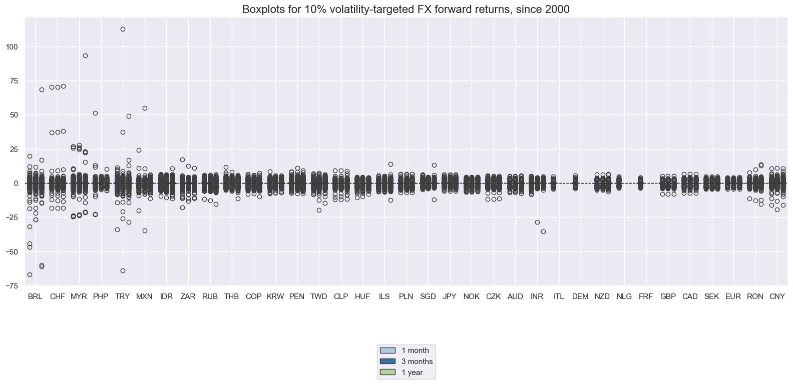
Volatility targeting makes a substantial difference in the long-term cumulative returns of forwards, even if the volatility target is close to the historical volatility of the exchange rate. This reflects two effects:

• Overtime risk of vol-targeted positions is reduced in times of turbulence and increased in quiet periods.

• Positions in low-vol currencies are increased and those in high-vol countries are reduced.

xcatx = ["FXXR_VT10", "FX06MXR_VT10", "FX01YXR_VT10"]
cidx = cids_fx

msp.view_timelines(
    dfd,
    xcats=xcatx,
    xcat_labels=["1-month forward", "6-months forward", "1-year forward"],
    cids=cidx,
    start="2000-01-01",
    title="Cumulative returns on vol-targeted FX forwards versus dominant benchmark for 1-month (blue), 6-month (orange) and 1-year (green) tenors",
    title_fontsize=30,
    legend_fontsize=20,
    cumsum=True,
    ncol=4,
    same_y=False,
    size=(12, 7),
    aspect=1.7,
    all_xticks=True,
)

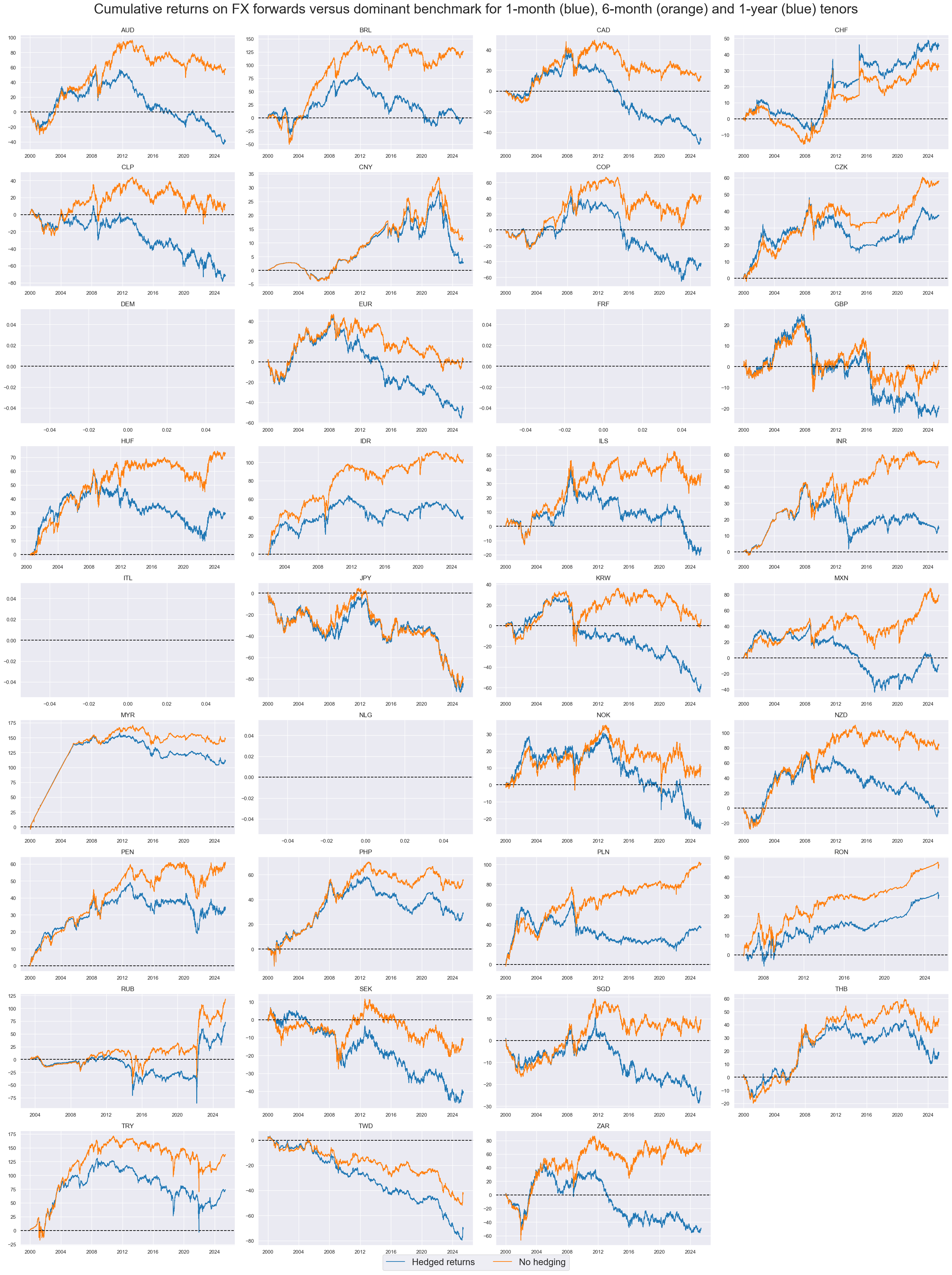
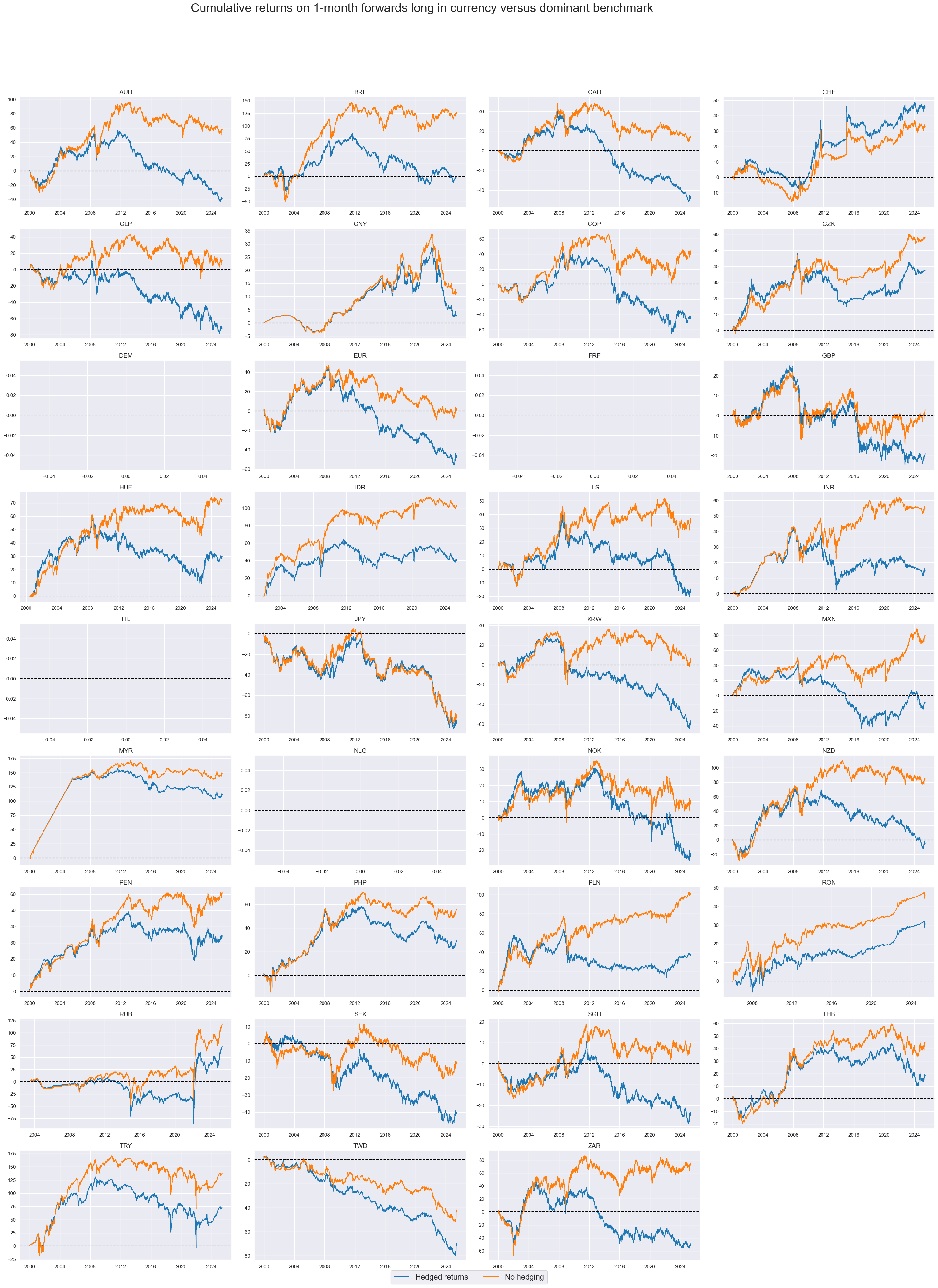
Hedged FX forward returns

Hedging against global directional risk would have greatly reduced the long-term cumulative return on many carry trades. This reflects that carry currencies often incur a high “beta”, i.e. high dependency of global risk market returns. Put simply, the idiosyncratic premium on carry currencies is often quite modest.

xcatx = ["FXXRHvGDRB_NSA", "FXXR_NSA"]
cidx = cids_fx

msp.view_timelines(
    dfd,
    xcats=xcatx,
    xcat_labels=["Hedged returns", "No hedging"],
    cids=cidx,
    start="2000-01-01",
    title="Cumulative returns on FX forwards versus dominant benchmark for 1-month (blue), 6-month (orange) and 1-year (blue) tenors",
    title_fontsize=30,
    legend_fontsize=20,
    cumsum=True,
    ncol=4,
    same_y=False,
    size=(12, 7),
    aspect=1.7,
    all_xticks=True,
)

msp.view_timelines(
    dfd,
    xcats=xcatx,
    cids=cidx,
    start="2000-01-01",
    title="Cumulative returns on 1-month forwards long in currency versus dominant benchmark",
    xcat_labels=["Hedged returns", "No hedging"],
    title_adj=1.03,
    title_xadj=0.45,
    title_fontsize=27,
    legend_fontsize=17,
    label_adj=0.075,
    cumsum=True,
    ncol=4,
    same_y=False,
    size=(12, 7),
    aspect=1.7,
    all_xticks=True,
)

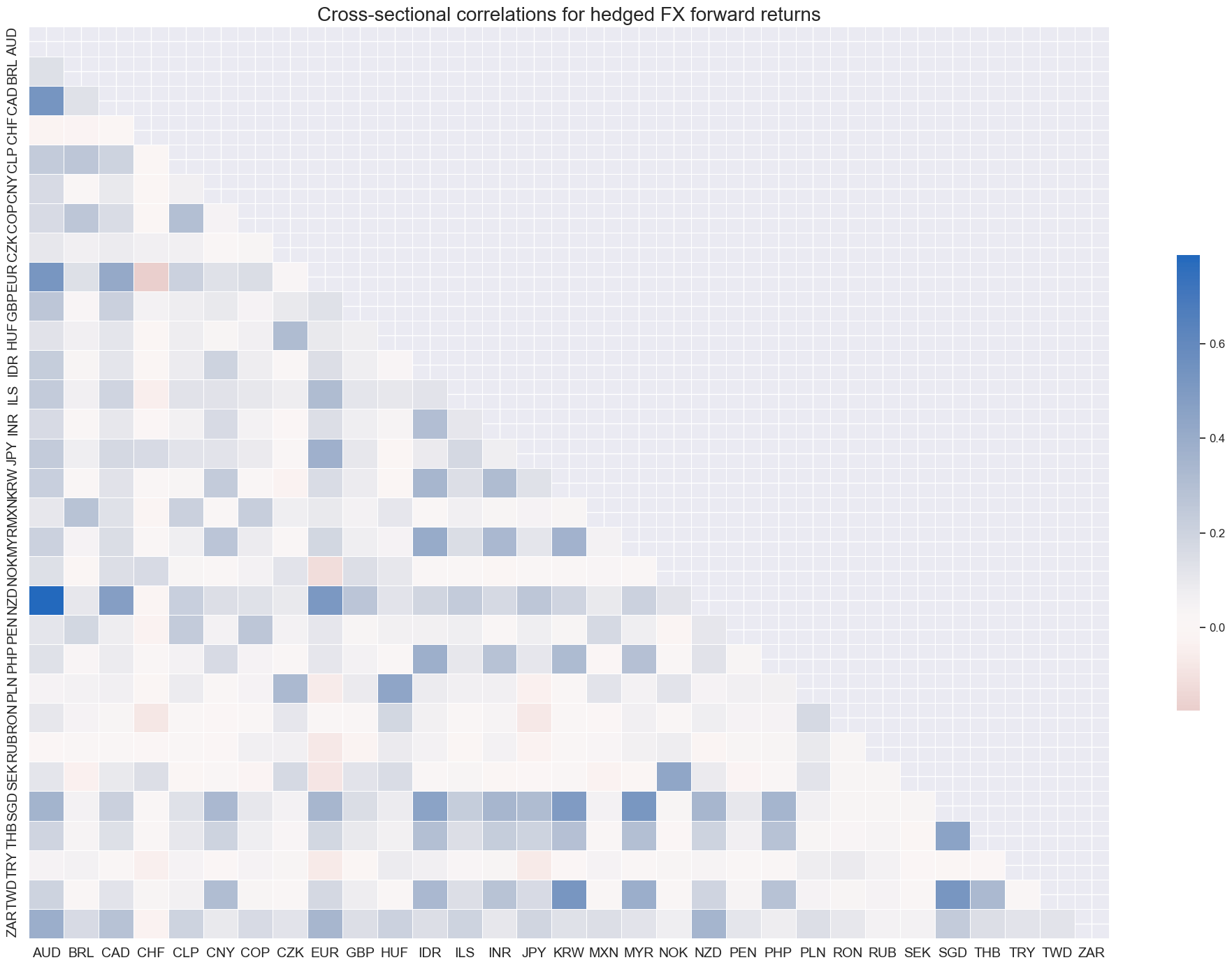
Hedging FX forward positions against global directional risk would have reduced and evened out most cross-currency correlation coefficients.

xcatx = "FXXRHvGDRB_NSA"
cidx = cids_fx

msp.correl_matrix(
    dfd,
    xcats=xcatx,
    cids=cidx,
    title="Cross-sectional correlations for hedged FX forward returns",
    size=(20, 14),
)

Importance

Research Links

“FX forward returns for 29 floating and convertible currencies since 1999 provide important empirical lessons. First, the long-term performance of FX returns has been dependent on economic structure and clearly correlated with forward-implied carry. The carry-return link has weakened considerably in the 2010s. Second, monthly returns for all currencies showed large and frequent outliers beyond the borders of a normal random distribution. Simple volatility targeting would not have mitigated this. Third, despite large fundamental differences, all carry and EM currencies have been positively correlated among themselves and with global risk benchmarks. Fourth, relative standard deviations across currencies have been predictable and partly structural. Hence, they have been important for scaling FX trades across small currencies.” Macrosynergy

Empirical Clues

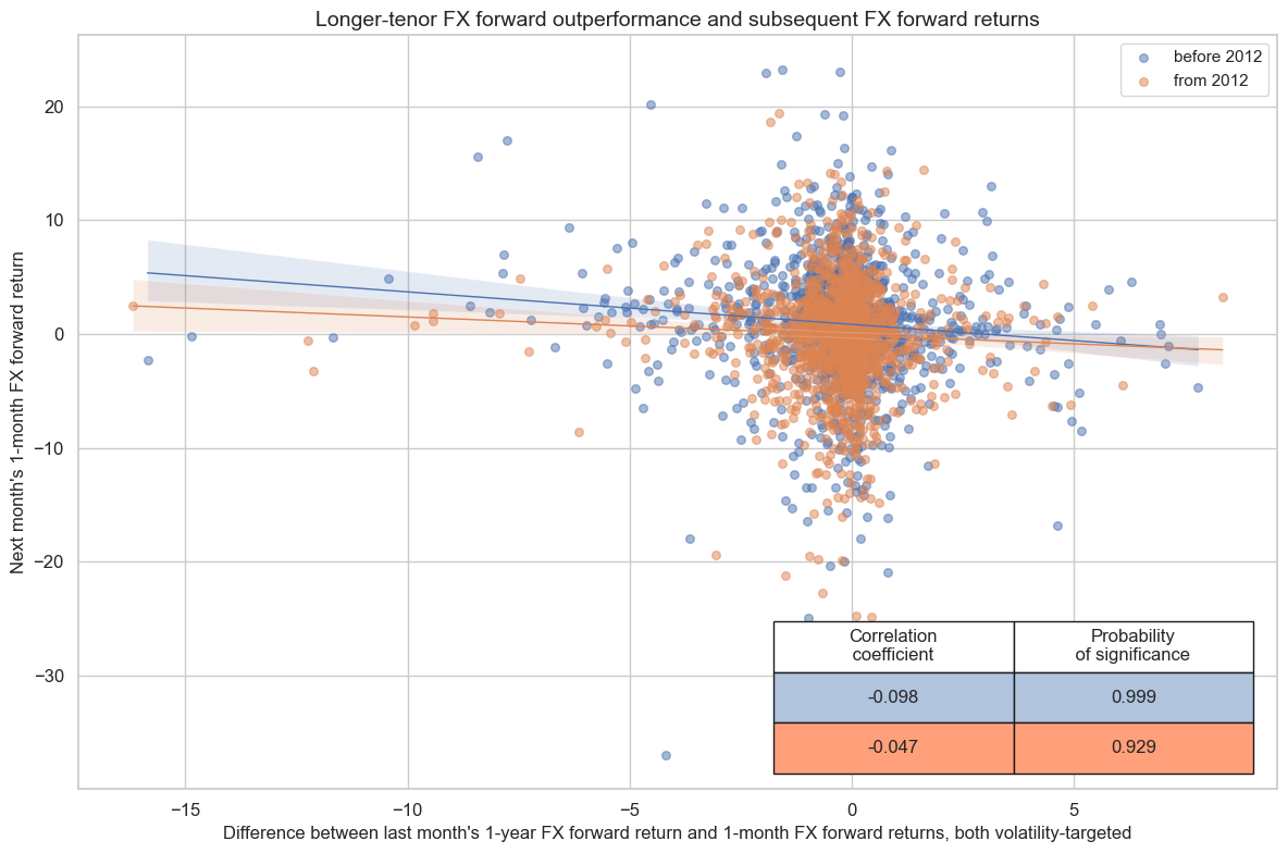
Historically, there has been a stable negative predictive correlation between the outperformance of the long-dated FX tenor and subsequent monthly or quarterly directional FX forward returns. The longer-dated tenor would typically outperform if 1-year interest rates in the local currency increased less than in the benchmark currency. This means that relative returns across tenor can be used as a proxy for relative changes in monetary policy expectations.

dfb = dfd[dfd["xcat"].isin(["FXTARGETED_NSA", "FXUNTRADABLE_NSA"])].loc[
    :, ["cid", "xcat", "real_date", "value"]
]
dfba = (
    dfb.groupby(["cid", "real_date"])
    .aggregate(value=pd.NamedAgg(column="value", aggfunc="max"))
    .reset_index()
)
dfba["xcat"] = "FXBLACK"
fxblack = msp.make_blacklist(dfba, "FXBLACK")

fx_calcs = [
    f"FX{tenor}XR_{adj}v1M = FX{tenor}XR_{adj} - FXXR_{adj}"
    for tenor in ["03M", "06M", "09M", "01Y"]
    for adj in ["NSA", "VT10"]
]
cidx = cids_fx

dfa = msp.panel_calculator(dfd, calcs=fx_calcs, cids=cidx)
dfd = msm.update_df(dfd, dfa)

xcatx = ["FX01YXR_VT10v1M", "FXXR_NSA"]
cidx = cids_fx

cr = msp.CategoryRelations(
    dfd,
    xcats=xcatx,
    cids=cidx,
    freq="Q",
    lag=1,
    xcat_aggs=["sum", "sum"],
    blacklist=fxblack,
    start="2000-01-01",
    years=None,
)

cr.reg_scatter(
    title="Longer-tenor FX forward outperformance and subsequent FX forward returns",
    labels=False,
    separator=2012,
    coef_box="lower right",
    xlab="Difference between last month's 1-year FX forward return and 1-month FX forward returns, both volatility-targeted",
    ylab="Next month's 1-month FX forward return",
)

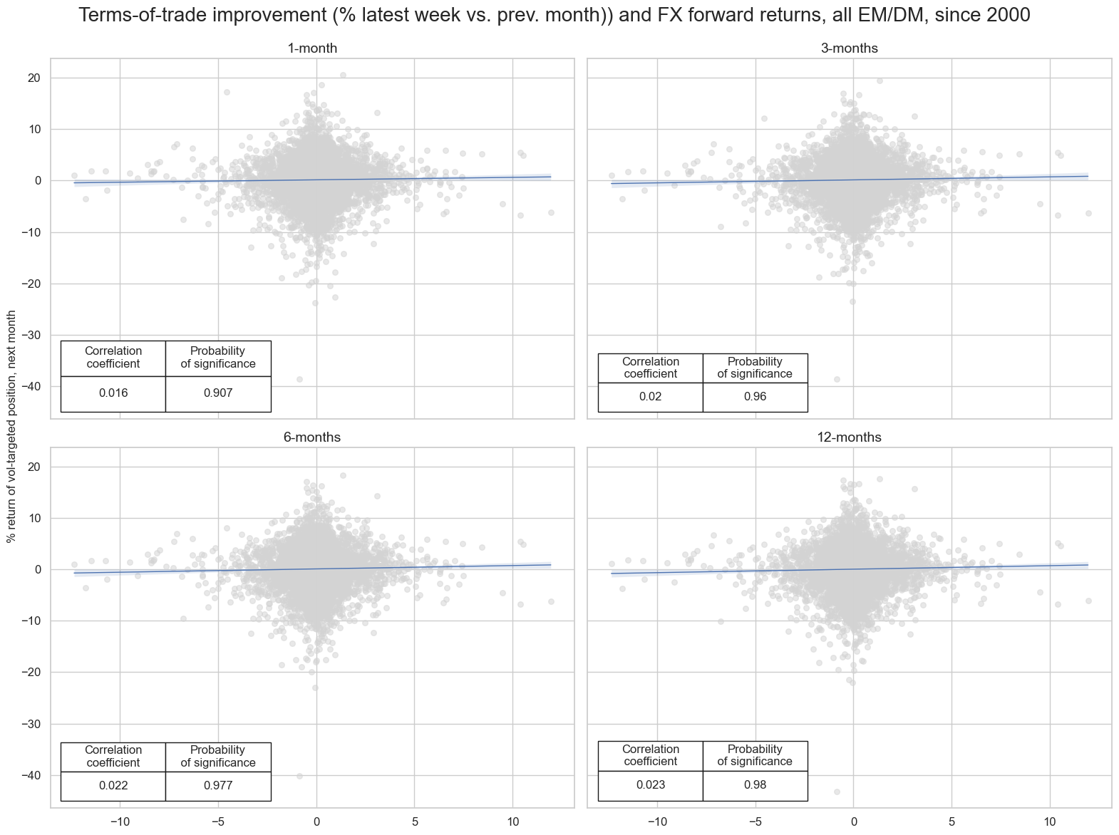
Terms-of-trade changes have been a short-term predictor of FX forward returns. This predictive power has been a little more signficant for longer FX forward tenors.

cidx = cids_fx

tenor_names = {
    "": "1-month",
    "03M": "3-months", 
    "06M": "6-months", 
    "01Y": "12-months"
}

ctot_ret_cr = {}
for tenor in ["", "03M", "06M", "01Y"]:
    ctot_ret_cr[tenor] = msp.CategoryRelations(
        dfd,
        xcats=["CTOT_NSA_P1W4WL1", f"FX{tenor}XR_VT10"],
        cids=cidx,
        freq="M",
        lag=1,
        xcat_aggs=["last", "sum"],
        blacklist=fxblack,
        start="2000-01-01",
        years=None,
    )

msv.multiple_reg_scatter(
        ctot_ret_cr.values(),
        title="Terms-of-trade improvement (% latest week vs. prev. month)) and FX forward returns, all EM/DM, since 2000",
        ylab="% return of vol-targeted position, next month",
        ncol=2,
        nrow=2,
        figsize=(16, 12),
        prob_est="map",
        coef_box="lower left", 
        subplot_titles=[tenor_names.get(k) for k in ctot_ret_cr.keys()],
     )

Appendix 1: Currency symbols

The word ‘cross-section’ refers to currencies, currency areas or economic areas. In alphabetical order, these are AUD (Australian dollar), BRL (Brazilian real), CAD (Canadian dollar), CHF (Swiss franc), CLP (Chilean peso), CNY (Chinese yuan renminbi), COP (Colombian peso), CZK (Czech Republic koruna), DEM (German mark), ESP (Spanish peseta), EUR (Euro), FRF (French franc), GBP (British pound), HKD (Hong Kong dollar), HUF (Hungarian forint), IDR (Indonesian rupiah), ITL (Italian lira), JPY (Japanese yen), KRW (Korean won), MXN (Mexican peso), MYR (Malaysian ringgit), NLG (Dutch guilder), NOK (Norwegian krone), NZD (New Zealand dollar), PEN (Peruvian sol), PHP (Phillipine peso), PLN (Polish zloty), RON (Romanian leu), RUB (Russian ruble), SEK (Swedish krona), SGD (Singaporean dollar), THB (Thai baht), TRY (Turkish lira), TWD (Taiwanese dollar), USD (U.S. dollar), ZAR (South African rand).