Equity index future returns #
This category group contains daily local-currency equity index future returns, as well as USD cash returns on synthetic equity indices for funded or unfunded investors. The returns are conceptually based on leveraged positions in the most liquid local currency-denominated indices.
Equity index future returns in % of notional #
Ticker : EQXR_NSA
Label : Equity index future returns in % of notional.
Definition : Return on front future of main country equity index, % of notional of the contract.
Notes :
-
The return is simply the % change of the futures price. The return calculation assumes rolling futures (from front to second) on IMM (international monetary markets) days.
-
See Appendix 1 for the list of equity indices used for each currency area in futures return calculations.
Unfunded USD returns on a synthetic foreign equity index in % of notional #
Ticker : EQXRUSD_NSA
Label : Unfunded USD cash return on a synthetic foreign equity index poistion, in % of notional.
Definition : Return in USD on an unfunded position for a synthetic foreign equity index, % of notional of the contract.
Notes :
-
The return is calculated as the sum of the % change of an index futures price, the daily interest in the local market, and the rate of appreciation of the local currency versus the U.S. dollar. From this we subtract the short U.S. dollar funding rate.
-
The return calculation assumes rolling futures (from front to second) on IMM (international monetary markets) days. FX spot rates used for conversion are based on the standard daily WMCO snapshots.
-
See Appendix 1 for the list of equity indices used for each currency area in futures return calculations.
Funded USD returns on a synthetic foreign equity index in % of notional #
Ticker : EQRUSD_NSA
Label : Funded USD cash return on a synthetic foreign equity index poistion, in % of notional.
Definition : Return in USD on a funded position for a synthetic foreign equity index, % of notional of the contract.
Notes :
-
The return is calculated as the sum of the % change of an index futures price, the daily interest in the local market, and the rate of appreciation of the local currency versus the U.S. dollar.
-
The return calculation assumes rolling futures (from front to second) on IMM (international monetary markets) days. FX spot rates used for conversion are based on the standard daily WMCO snapshots.
-
See Appendix 1 for the list of equity indices used for each currency area in futures return calculations.
Alternative equity index future returns in % of notional #
Ticker : EQNASDAQXR_NSA / EQRUSSELLXR_NSA / EQTOPIXXR_NSA / EQHANGSENGXR_NSA
Label : Equity index future returns in % of notional: NASDAQ 100 / Russell 2000 / TOPIX / Hang Seng.
Definition : Return on front future of alternative country equity index, % of notional of the contract: NASDAQ 100 / Russell 2000 / TOPIX / Hang Seng.
Notes :
-
Alternative indices are not the main equity index of the country but are available for suplementary analyses.
-
See Appendix 2 for the list of alternative equity indices used. Alternative indices are available for HKD, JPY, and USD.
-
See the important notes under “Equity index future returns in % of notional” (
EQXR_NSA).
Unfunded USD returns on alternative synthetic foreign equity index in % of notional #
Ticker : EQNASDAQXRUSD_NSA / EQRUSSELLXRUSD_NSA / EQTOPIXXRUSD_NSA / EQHANGSENGXRUSD_NSA
Label : Unfunded USD cash return on alternative synthetic foreign equity index poistion, in % of notional: NASDAQ 100 / Russell 2000 / TOPIX / Hang Seng.
Definition : Return in USD on an unfunded position for synthetic foreign equity alternative index, % of notional of the contract: NASDAQ 100 / Russell 2000 / TOPIX / Hang Seng.
Notes :
-
Alternative indices are not the main equity index of the country but are available for suplementary analyses.
-
See Appendix 2 for the list of alternative equity indices used. Alternative indices are available for HKD, JPY, and USD.
-
See the important notes under “Unfunded USD returns on a synthetic foreign equity index in % of notional” (
EQXRUSD_NSA).
Funded USD returns on alternative synthetic foreign equity index in % of notional #
Ticker : EQNASDAQRUSD_NSA / EQRUSSELLRUSD_NSA / EQTOPIXRUSD_NSA / EQHANGSENGRUSD_NSA
Label : Funded USD cash return on alternative synthetic foreign equity index poistion, in % of notional: NASDAQ 100 / Russell 2000 / TOPIX / Hang Seng.
Definition : Return in USD on a funded position for synthetic foreign equity alternative index, % of notional of the contract: NASDAQ 100 / Russell 2000 / TOPIX / Hang Seng.
Notes :
-
Alternative indices are not the main equity index of the country but are available for suplementary analyses.
-
See Appendix 2 for the list of alternative equity indices used. Alternative indices are available for HKD, JPY, and USD.
-
See the important notes under “Funded USD returns on a synthetic foreign equity index in % of notional” (
EQRUSD_NSA).
Vol-targeted equity index future returns #
Ticker : EQXR_VT10
Label : Equity index future return for 10% vol target.
Definition : Return on front future of main country equity index, % of risk capital on position scaled to 10% (annualized) volatility target.
Notes :
-
Positions are scaled to a 10% volatility target based on the historic standard deviation for an exponential moving average with a half-life of 11 days. Positions are rebalanced at the end of each month.
-
See the important notes under “Equity index future returns in % of notional” (
EQXR_NSA).
Vol-targeted unfunded USD returns on a synthetic foreign equity index #
Ticker : EQXRUSD_VT10
Label : Unfunded USD cash return on a synthetic foreign equity index poistion, in % of notional.
Definition : Return in USD on an unfunded position for a synthetic foreign equity index, % of notional of the contract.
Notes :
-
Positions are scaled to a 10% volatility target based on the historic standard deviation for an exponential moving average with a half-life of 11 days. Positions are rebalanced at the end of each month.
-
Note that the volatility scaling is applied to the unfunded USD returns on a synthetic foreign equity index in % of notional. This is different from vol-scaling the local-currency index returns and then accounting for spot FX changes.
-
See the important notes under “Unfunded USD returns on a synthetic foreign equity index in % of notional” (
EQXRUSD_NSA).
Vol-targeted funded USD returns on a synthetic foreign equity index #
Ticker : EQRUSD_VT10
Label : Funded USD cash return on a synthetic foreign equity index poistion, for 10% vol target..
Definition : Return in USD on a funded position for a synthetic foreign equity index, % of risk capital on position scaled to 10% (annualized) volatility target.
Notes :
-
Positions are scaled to a 10% volatility target based on the historic standard deviation for an exponential moving average with a half-life of 11 days. Positions are rebalanced at the end of each month.
-
Note that the volatility scaling is applied to the funded USD returns on a synthetic foreign equity index in % of notional. This is different from vol-scaling the local-currency index returns and then accounting for spot FX changes.
-
See the important notes under “Funded USD returns on a synthetic foreign equity index in % of notional” (
EQRUSD_NSA).
Vol-targeted alternative equity index future return #
Ticker : EQNASDAQXR_VT10 / EQRUSSELLXR_VT10 / EQTOPIXXR_VT10 / EQHANGSENGXR_VT10
Label : Equity index future return for 10% vol target: NASDAQ 100 / Russell 2000 / TOPIX / Hang Seng.
Definition : Return on front future of alternative country equity index, % of risk capital on position scaled to 10% (annualized) volatility target: NASDAQ 100 / Russell 2000 / TOPIX / Hang Seng.
Notes :
-
Positions are scaled to a 10% volatility target based on the historic standard deviation for an exponential moving average with a half-life of 11 days. Positions are rebalanced at the end of each month.
-
See Appendix 2 for the list of alternative equity indices used. Alternative indices are available for HKD, JPY, and USD.
-
See the important notes under “Equity index future returns in % of notional” (
EQXR_NSA).
Vol-targeted unfunded USD returns on alternative synthetic foreign equity index #
Ticker : EQNASDAQXRUSD_VT10 / EQRUSSELLXRUSD_VT10 / EQTOPIXXRUSD_VT10 / EQHANGSENGXRUSD_VT10
Label : Unfunded USD cash return on alternative synthetic foreign equity index poistion, for 10% vol target: NASDAQ 100 / Russell 2000 / TOPIX / Hang Seng.
Definition : Return in USD on an unfunded position for synthetic foreign equity alternative index, % of risk capital on position scaled to 10% (annualized) volatility target: NASDAQ 100 / Russell 2000 / TOPIX / Hang Seng.
Notes :
-
Alternative indices are not the main equity index of the country but are available for suplementary analyses.
-
See Appendix 2 for the list of alternative equity indices used. Alternative indices are available for HKD, JPY, and USD.
Vol-targeted funded USD returns on alternative synthetic foreign equity index #
Ticker : EQNASDAQRUSD_VT10 / EQRUSSELLRUSD_VT10 / EQTOPIXRUSD_VT10 / EQHANGSENGRUSD_VT10
Label : Funded USD cash return on alternative synthetic foreign equity index poistion, for 10% vol target: NASDAQ 100 / Russell 2000 / TOPIX / Hang Seng.
Definition : Return in USD on a funded position for synthetic foreign equity alternative index, % of risk capital on position scaled to 10% (annualized) volatility target: NASDAQ 100 / Russell 2000 / TOPIX / Hang Seng.
Notes :
-
Alternative indices are not the main equity index of the country but are available for suplementary analyses.
-
See Appendix 2 for the list of alternative equity indices used. Alternative indices are available for HKD, JPY, and USD.
Imports #
Only the standard Python data science packages and the specialized
macrosynergy
package are needed.
import os
import numpy as np
import pandas as pd
import matplotlib.pyplot as plt
import seaborn as sns
import math

import json
import yaml

import macrosynergy.management as msm
import macrosynergy.panel as msp
import macrosynergy.signal as mss
import macrosynergy.pnl as msn


from macrosynergy.download import JPMaQSDownload

from timeit import default_timer as timer
from datetime import timedelta, date, datetime

import warnings

warnings.simplefilter("ignore")
The
JPMaQS
indicators we consider are downloaded using the J.P. Morgan Dataquery API interface within the
macrosynergy
package. This is done by specifying
ticker strings
, formed by appending an indicator category code
<category>
to a currency area code
<cross_section>
. These constitute the main part of a full quantamental indicator ticker, taking the form
DB(JPMAQS,<cross_section>_<category>,<info>)
, where
<info>
denotes the time series of information for the given cross-section and category. The following types of information are available:
-
valuegiving the latest available values for the indicator -
eop_lagreferring to days elapsed since the end of the observation period -
mop_lagreferring to the number of days elapsed since the mean observation period -
gradedenoting a grade of the observation, giving a metric of real time information quality.
After instantiating the
JPMaQSDownload
class within the
macrosynergy.download
module, one can use the
download(tickers,start_date,metrics)
method to easily download the necessary data, where
tickers
is an array of ticker strings,
start_date
is the first collection date to be considered and
metrics
is an array comprising the times series information to be downloaded.
# Cross-sections of interest

cids_dmeq = ["AUD", "CAD", "CHF", "EUR", "GBP", "JPY", "SEK", "USD"]
cids_eueq = ["DEM", "ESP", "FRF", "ITL", "NLG"]
cids_aseq = ["CNY", "HKD", "INR", "KRW", "MYR", "SGD", "THB", "TWD"]
cids_exeq = ["BRL", "TRY", "ZAR"]
cids_nueq = ["MXN", "PLN"]

cids = sorted(cids_dmeq + cids_eueq + cids_aseq + cids_exeq + cids_nueq)
main = ["EQXR_NSA", "EQXR_VT10", "EQRUSD_NSA", "EQRUSD_VT10", "EQXRUSD_NSA", "EQXRUSD_VT10"]

econ = ["BXBGDPRATIO_NSA_12MMA", "CABGDPRATIO_NSA_12MMA"]  # economic context

mark = [
    "EQCRR_NSA",
    "EQCRR_VT10",
    "FXXR_NSA",
    "FXTARGETED_NSA",
    "FXUNTRADABLE_NSA",
]  # market links

xcats = main + econ + mark
# Download series from J.P. Morgan DataQuery by tickers

start_date = "1990-01-01"
tickers = [cid + "_" + xcat for cid in cids for xcat in xcats]
alt_tickers = [
    "USD_EQNASDAQXR_NSA",
    "USD_EQNASDAQXR_VT10",
    "USD_EQNASDAQRUSD_NSA",
    "USD_EQNASDAQRUSD_VT10",
    "USD_EQNASDAQXRUSD_NSA",
    "USD_EQNASDAQXRUSD_VT10",

    "USD_EQRUSSELLXR_NSA",
    "USD_EQRUSSELLXR_VT10",
    "USD_EQRUSSELLRUSD_NSA",
    "USD_EQRUSSELLRUSD_VT10",
    "USD_EQRUSSELLXRUSD_NSA",
    "USD_EQRUSSELLXRUSD_VT10",

    "JPY_EQTOPIXXR_NSA",
    "JPY_EQTOPIXXR_VT10",
    "JPY_EQTOPIXRUSD_NSA",
    "JPY_EQTOPIXRUSD_VT10",
    "JPY_EQTOPIXXRUSD_NSA",
    "JPY_EQTOPIXXRUSD_VT10",

    "HKD_EQHANGSENGXR_NSA",
    "HKD_EQHANGSENGXR_VT10",
    "HKD_EQHANGSENGRUSD_NSA",
    "HKD_EQHANGSENGRUSD_VT10",
    "HKD_EQHANGSENGXRUSD_NSA",
    "HKD_EQHANGSENGXRUSD_VT10",
]
tickers = tickers + alt_tickers
print(f"Maximum number of tickers is {len(tickers)}")

# Retrieve credentials

client_id: str = os.getenv("DQ_CLIENT_ID")
client_secret: str = os.getenv("DQ_CLIENT_SECRET")

# Download from DataQuery

with JPMaQSDownload(client_id=client_id, client_secret=client_secret) as downloader:
    start = timer()
    assert downloader.check_connection()
    df = downloader.download(
        tickers=tickers,
        start_date=start_date,
        metrics=["value", "eop_lag", "mop_lag", "grading"],
        suppress_warning=True,
        show_progress=True,
    )
    end = timer()

dfd = df

print("Download time from DQ: " + str(timedelta(seconds=end - start)))
Maximum number of tickers is 362
Downloading data from JPMaQS.
Timestamp UTC:  2025-09-25 16:41:25
Connection successful!
Requesting data: 100%|██████████████████████████████████████████████████| 73/73 [00:15<00:00,  4.63it/s]
Downloading data: 100%|█████████████████████████████████████████████████| 73/73 [00:39<00:00,  1.83it/s]
Some expressions are missing from the downloaded data. Check logger output for complete list.
68 out of 1448 expressions are missing. To download the catalogue of all available expressions and filter the unavailable expressions, set `get_catalogue=True` in the call to `JPMaQSDownload.download()`.
Download time from DQ: 0:01:06.883880
Availability #
cids_exp = cids  # cids expected in category panels
msm.missing_in_df(dfd, xcats=main, cids=cids_exp)
No missing XCATs across DataFrame.
Missing cids for EQRUSD_NSA:    []
Missing cids for EQRUSD_VT10:   []
Missing cids for EQXRUSD_NSA:   []
Missing cids for EQXRUSD_VT10:  []
Missing cids for EQXR_NSA:      []
Missing cids for EQXR_VT10:     []
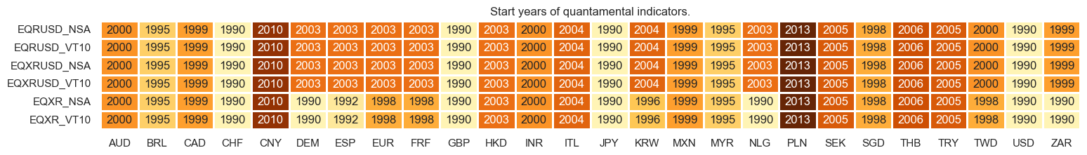
For most countries the series start in the 1990s, but China’s and Poland’s return series only begin the 2010s.
For the explanation of currency symbols, which are related to currency areas or countries for which categories are available, please view Appendix 3 .
xcatx = main
cidx = cids_exp

dfx = msm.reduce_df(dfd, xcats=xcatx, cids=cidx)
dfs = msm.check_startyears(
    dfx,
)
msm.visual_paneldates(dfs, size=(18, 2))

print("Last updated:", date.today())
Last updated: 2025-09-25
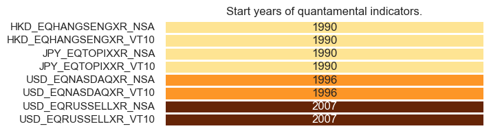
Alternative indicators are available for HKD, JPY and USD. They enable suplementary analyses with different focuses when compared to the country’s main index (small caps, broader/narrower coverage, etc.). All the alternative indices series are available since the 2000s.
alt_cats = [
    "EQNASDAQXR_NSA",
    "EQNASDAQXR_VT10",
    "EQRUSSELLXR_NSA",
    "EQRUSSELLXR_VT10",
    "EQTOPIXXR_NSA",
    "EQTOPIXXR_VT10",
    "EQHANGSENGXR_NSA",
    "EQHANGSENGXR_VT10",
]

dfx = msm.reduce_df(dfd, xcats=alt_cats, cids=cidx)
dfs = msm.check_startyears(
    dfx,
)

# Creating the dataframe for alternative indices
dfs_alt = pd.DataFrame(
    [
        {
            f"{index}_{col}": dfs.loc[index, col]
            for index in dfs.index
            for col in dfs.columns
            if not pd.isna(dfs.loc[index, col])
        }
    ]
)
dfs_alt["idx"] = ""
dfs_alt = dfs_alt.set_index("idx")

msm.visual_paneldates(dfs_alt, size=(6, 2))

print("Last updated:", date.today())
Last updated: 2025-09-25
xcatx = main
cidx = cids_exp

plot = msp.heatmap_grades(
    dfd,
    xcats=xcatx,
    cids=cidx,
    size=(18, 2),
    title=f"Average vintage grades from {start_date} onwards",
)
History #
Equity index future returns in % of notional #
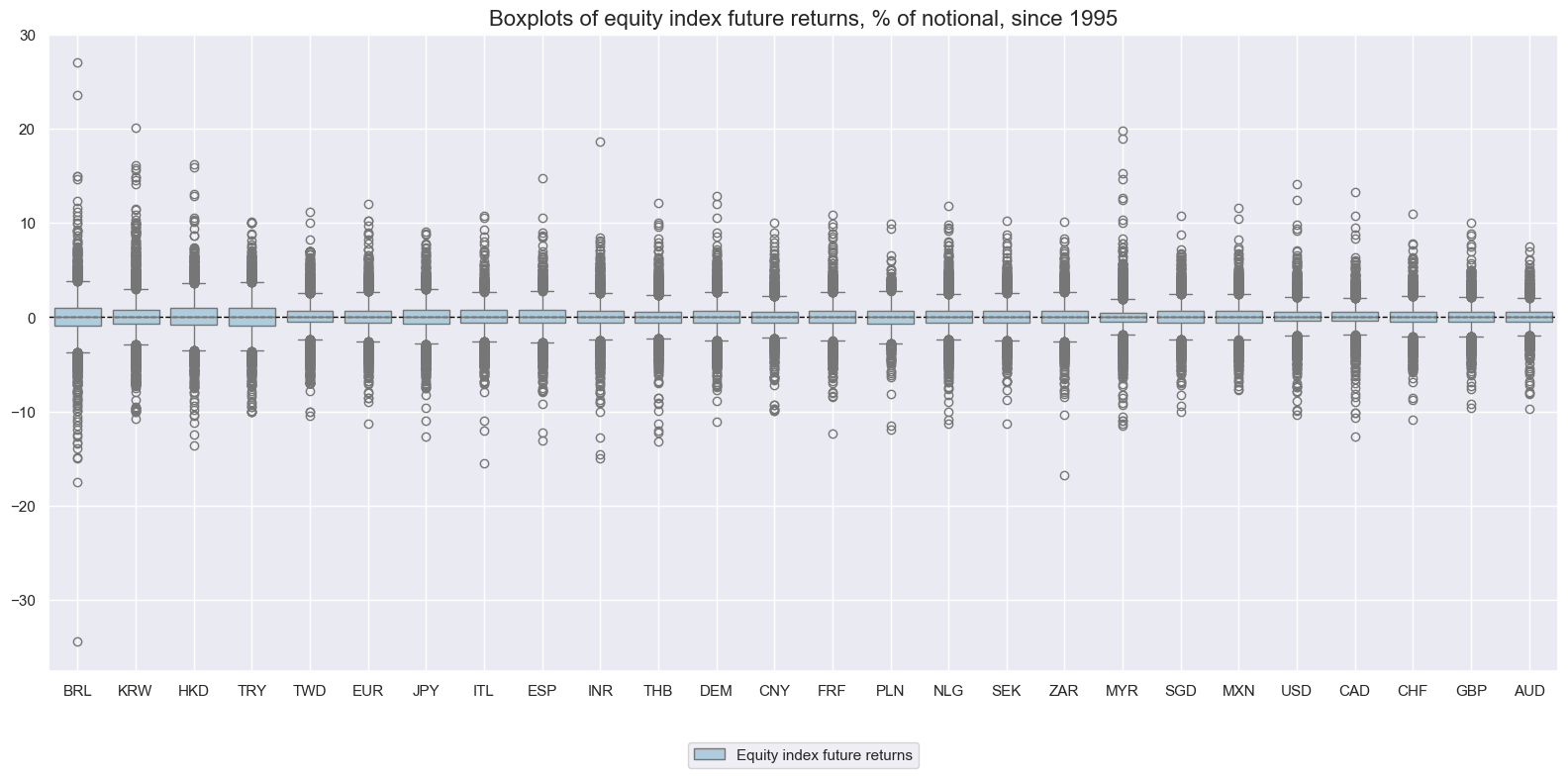
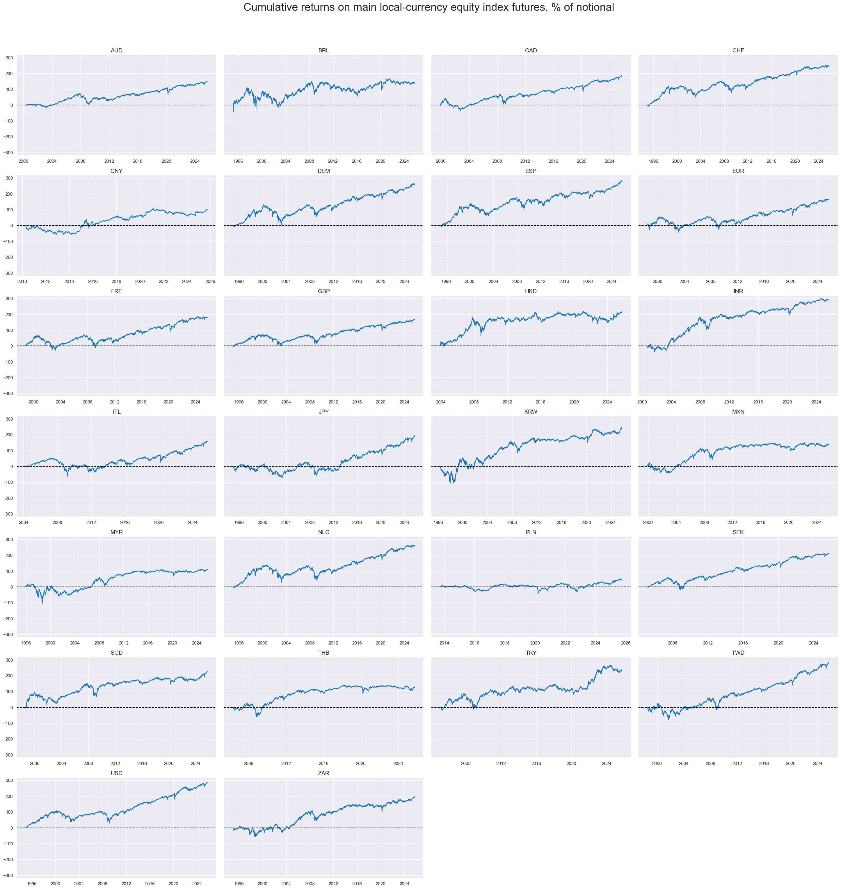
Long-term return distributions have been more homogeneous across currency areas than the distributions of FX or interest rate swap returns.
xcatx = ["EQXR_NSA"]
cidx = cids_exp
start_date="1995-01-01"

msp.view_ranges(
    dfd,
    xcats=xcatx,
    cids=cidx,
    sort_cids_by="std",
    start=start_date,
    kind="box",
    title="Boxplots of equity index future returns, % of notional, since 1995",
    xcat_labels=["Equity index future returns"],
    size=(16, 8),
)
xcatx = ["EQXR_NSA"]
cidx = cids_exp

msp.view_timelines(
    dfd,
    xcats=xcatx,
    cids=cidx,
    start=start_date,
    title="Cumulative returns on main local-currency equity index futures, % of notional",
    title_fontsize=27,
    title_adj=1.02,
    title_xadj=0.51,
    cumsum=True,
    ncol=4,
    same_y=True,
    size=(12, 7),
    aspect=1.7,
    all_xticks=True,
)
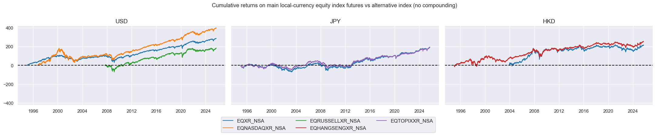
Despite their similarities, alternative indices provide different lenses to evaluate the market, revealing distinct return dynamics throughout their history - such as the recent steep growth of NASDAQ 100 returns when compared to S&P 500, and the shift between TOPIX and Nikkei 250 returns after 2008.
msp.view_timelines(
    dfd,
    xcats=["EQXR_NSA", "EQNASDAQXR_NSA", "EQRUSSELLXR_NSA", "EQHANGSENGXR_NSA", "EQTOPIXXR_NSA"],
    cids=['USD', 'JPY', 'HKD'],
    start=start_date,
    title="Cumulative returns on main local-currency equity index futures vs alternative index (no compounding)",
    title_fontsize=13,
    title_adj=1.02,
    title_xadj=0.51,
    cumsum=True,
    ncol=4,
    same_y=True,
    size=(6, 3.5),
    aspect=1.7,
    all_xticks=True,
)
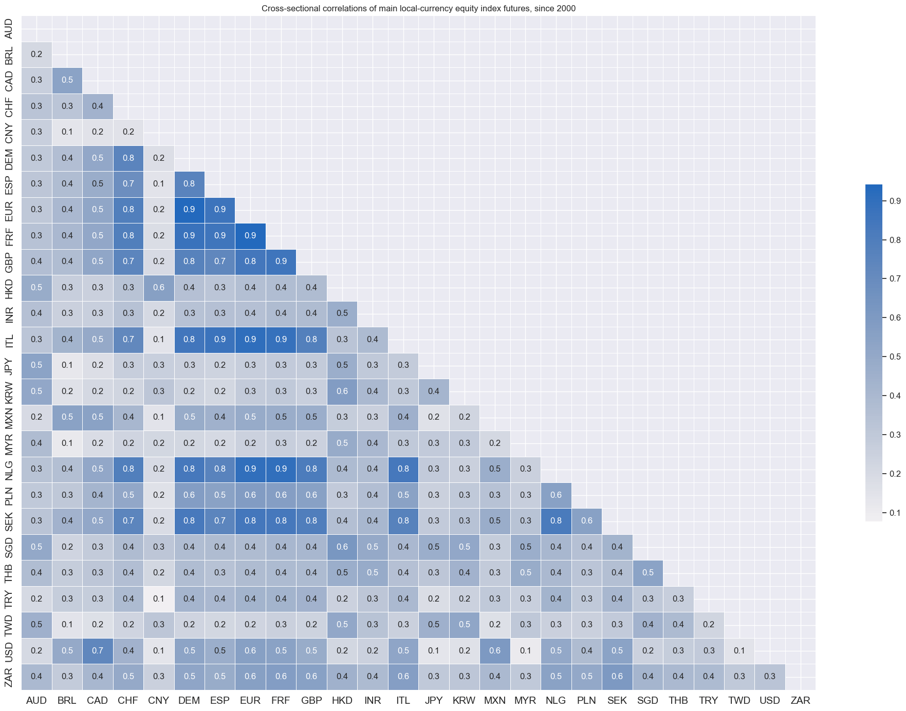
Unsurprisingly, cross-country correlations of daily equity future returns have been all positive since 2000. China displayed the lowest correlation with other countries.
xcatx = "EQXR_NSA"
cidx = cids_exp

msp.correl_matrix(
    dfd,
    xcats=xcatx,
    cids=cidx,
    title="Cross-sectional correlations of main local-currency equity index futures, since 2000",
    size=(20, 14),
    annot=True,
    fmt=".1f",
)
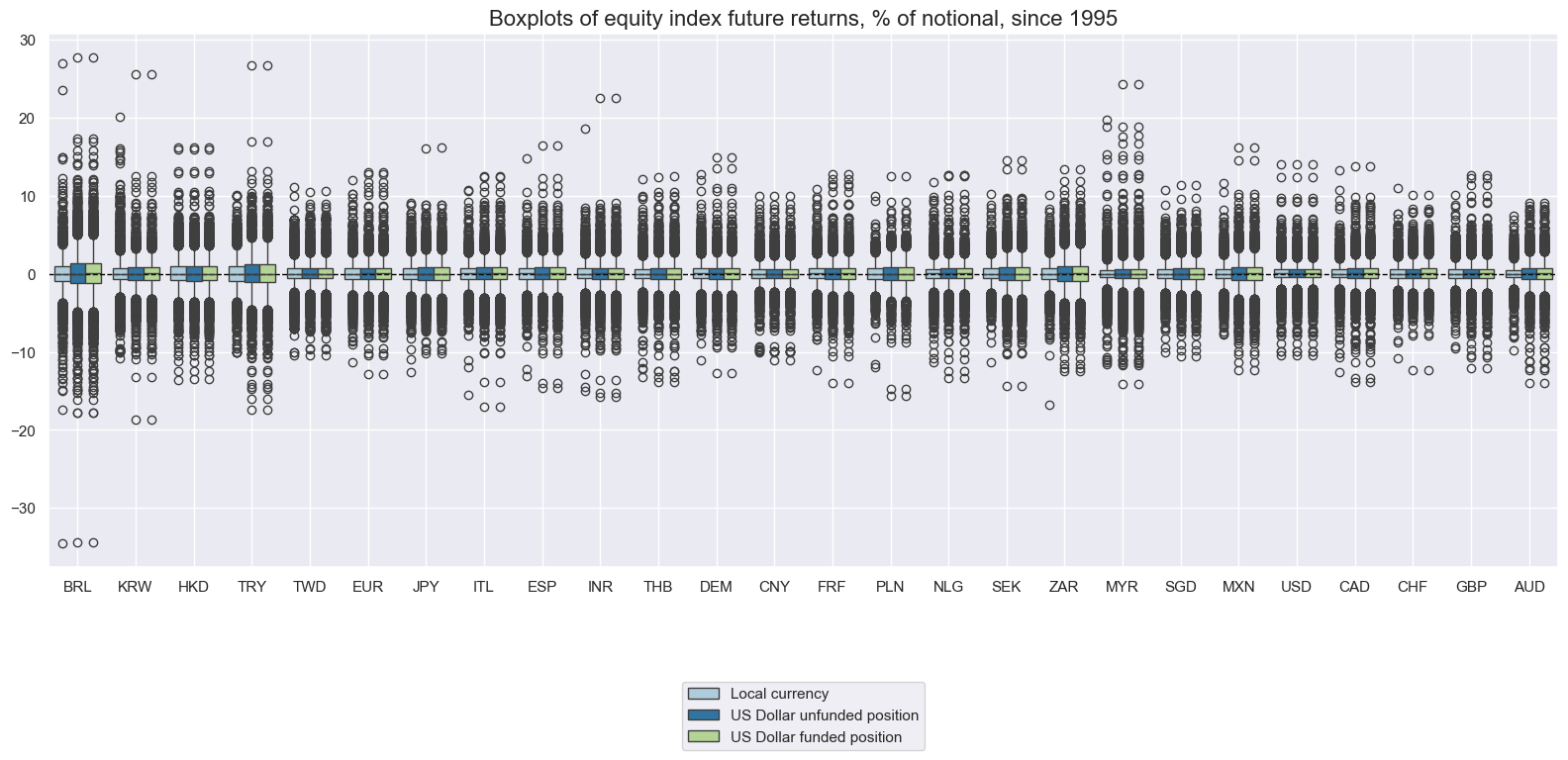
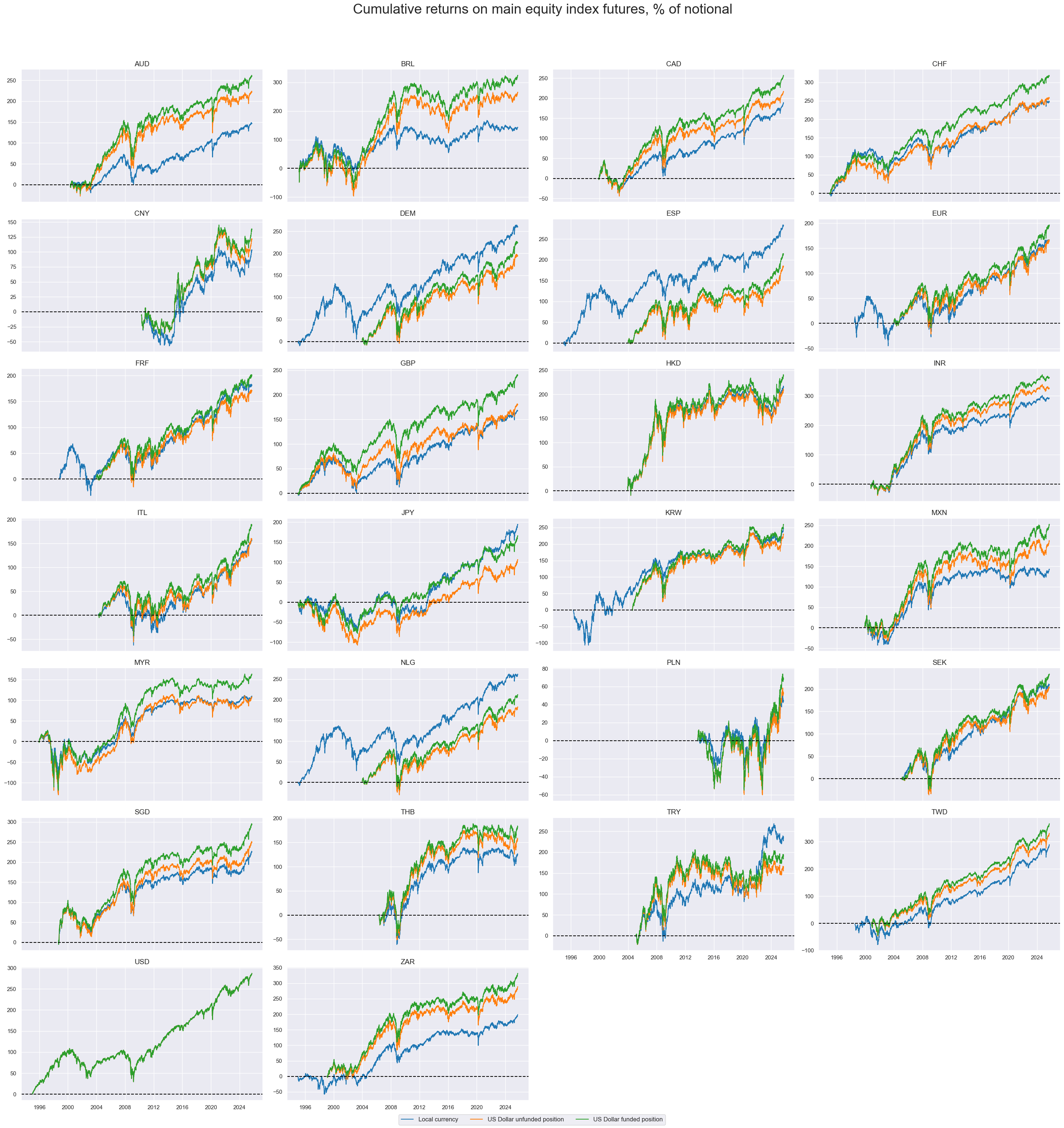
Funded and unfunded USD returns on a synthetic foreign equity index in % of notional #
Differences in distribution of daily equity future excess returns emerge when looking at investors with localy currency exposures vs funded or unfunded USD positions. In particular, tails and extreme movements seem to differ, with USD-denominated returns showing additional volatility for some areas like BRL, KRW, and TRY.
xcatx = ["EQXR_NSA", "EQXRUSD_NSA", "EQRUSD_NSA"]
cidx = cids_exp
start_date="1995-01-01"

msp.view_ranges(
    dfd,
    xcats=xcatx,
    cids=cidx,
    sort_cids_by="std",
    start=start_date,
    kind="box",
    title="Boxplots of equity index future returns, % of notional, since 1995",
    xcat_labels=["Local currency", "US Dollar unfunded position", "US Dollar funded position"],
    size=(16, 8),
)
FX dynamics matter as local currency evolution vs USD has both cyclical and long-term implications for asset allocators and investors.
xcatx = ["EQXR_NSA", "EQXRUSD_NSA", "EQRUSD_NSA",]
cidx = cids_exp

msp.view_timelines(
    dfd,
    xcats=xcatx,
    cids=cidx,
    start=start_date,
    title="Cumulative returns on main equity index futures, % of notional",
    title_fontsize=27,
    title_adj=1.02,
    title_xadj=0.51,
    cumsum=True,
    ncol=4,
    same_y=False,
    size=(12, 7),
    aspect=1.7,
    all_xticks=False,
    xcat_labels=["Local currency", "US Dollar unfunded position", "US Dollar funded position"]
)
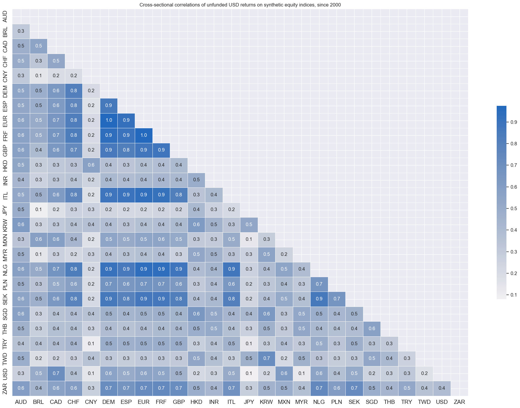
Daily correlations of USD returns on funded and unfunded synthetic positions remain positive, driven by the underlying equity index dynamics. FX appreciation vs USD adds further positive co-movement across markets.
xcatx = "EQXRUSD_NSA"
cidx = cids_exp

msp.correl_matrix(
    dfd,
    xcats=xcatx,
    cids=cidx,
    title="Cross-sectional correlations of unfunded USD returns on synthetic equity indices, since 2000",
    size=(20, 14),
    annot=True,
    fmt=".1f",
)
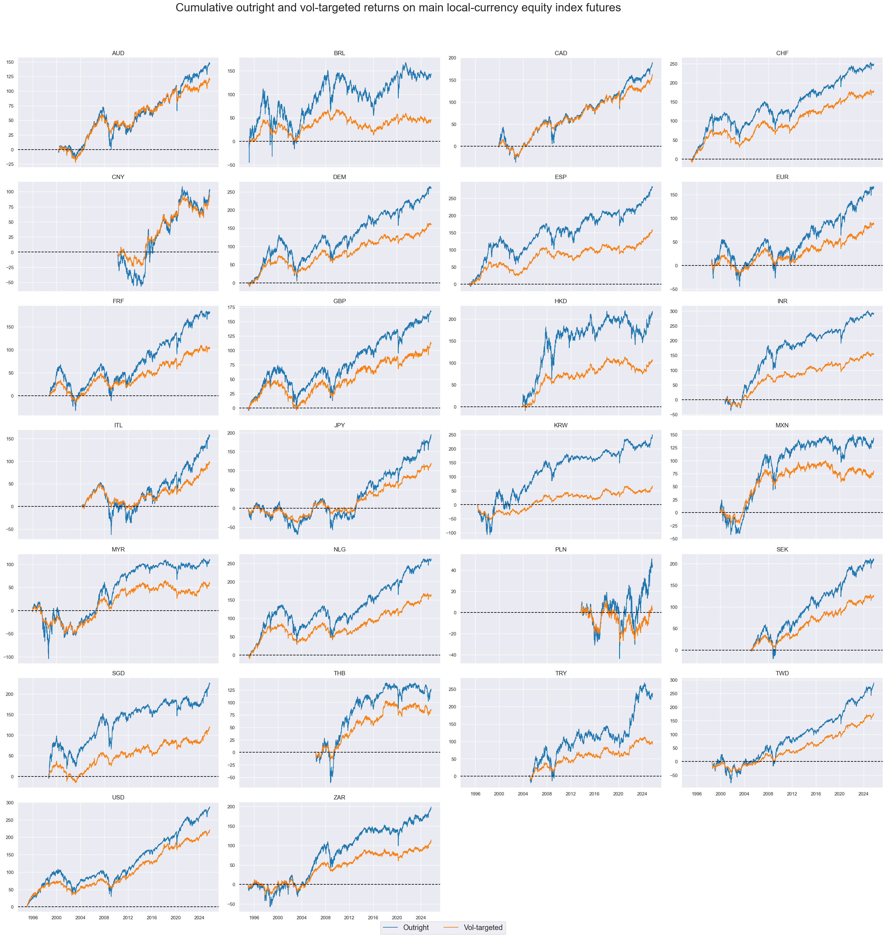
Vol-targeted equity index future returns #
Volatility targeting reduces the relative cumulative performance of most emerging market indices relative to the developed world.
xcatx = ["EQXR_NSA", "EQXR_VT10"]
cidx = cids_exp

msp.view_timelines(
    dfd,
    xcats=xcatx,
    cids=cidx,
    start=start_date,
    title="Cumulative outright and vol-targeted returns on main local-currency equity index futures",
    xcat_labels=["Outright", "Vol-targeted"],
    title_adj=1.02,
    title_xadj=0.45,
    legend_fontsize=17,
    label_adj=0.075,
    title_fontsize=27,
    cumsum=True,
    ncol=4,
    same_y=False,
    size=(12, 7),
    aspect=1.7,
    all_xticks=False,
)
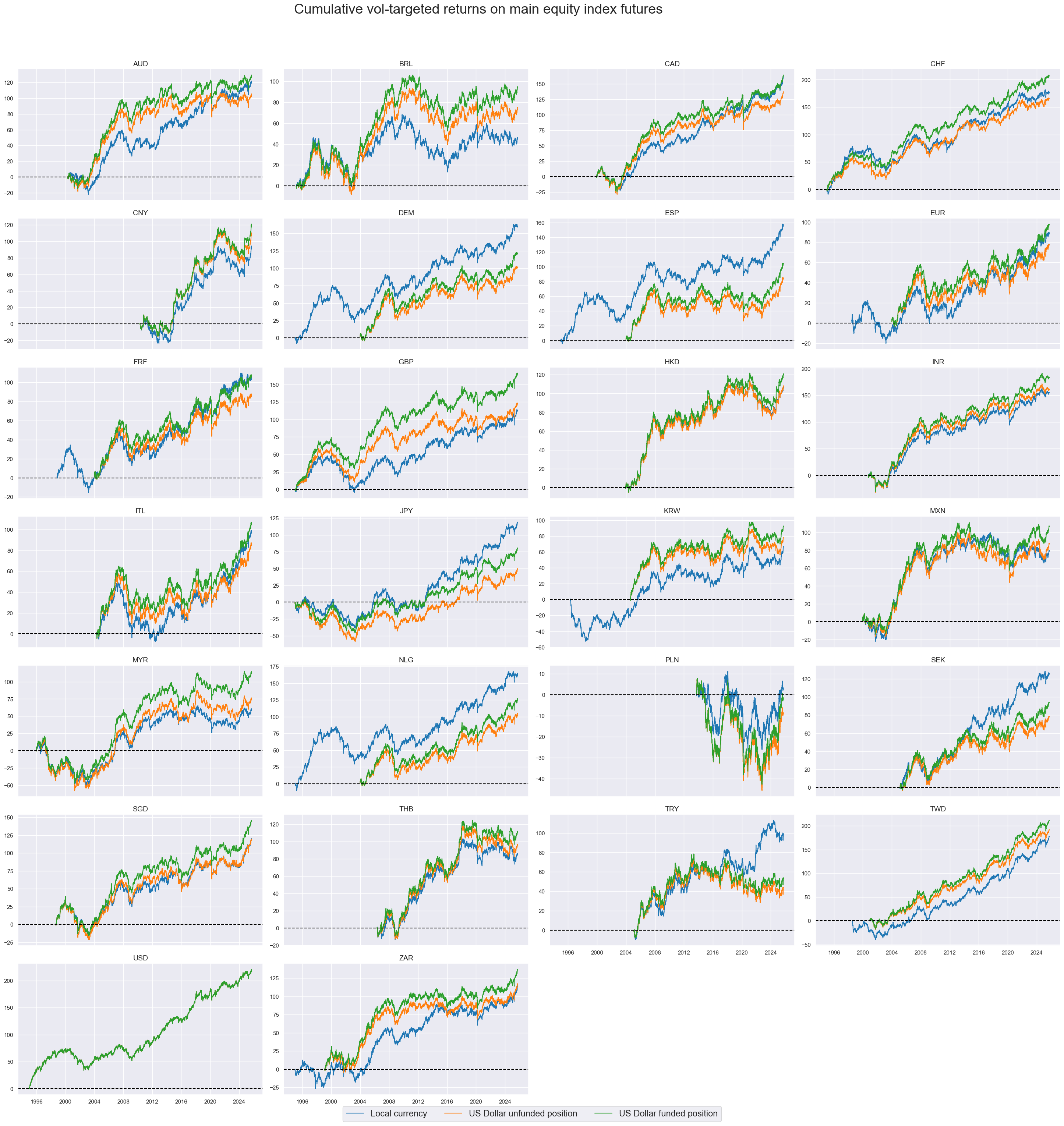
Incorporating FX dynamics into equity futures returns reveal striking differences, especially in emerging markets where the FX volaility is more pronounced.
Temporary deviations vs the local-currency vol-targeted index returns are also present in developed markets such as AUD, CHF, and EUR, highlighting the necessity to incorporate foreign exchange into global equity investors allocation decisions.
xcatx = ["EQXR_VT10", "EQXRUSD_VT10", "EQRUSD_VT10"]
cidx = cids_exp

msp.view_timelines(
    dfd,
    xcats=xcatx,
    cids=cidx,
    start=start_date,
    title="Cumulative vol-targeted returns on main equity index futures",
    xcat_labels=["Local currency", "US Dollar unfunded position", "US Dollar funded position"],
    title_adj=1.02,
    title_xadj=0.45,
    legend_fontsize=17,
    label_adj=0.075,
    title_fontsize=27,
    cumsum=True,
    ncol=4,
    same_y=False,
    size=(12, 7),
    aspect=1.7,
    all_xticks=False,
)
Importance #
Research Links #
“The vast range of academically researched equity return anomalies can be condensed into five categories: (1) return momentum, (2) outperformance of high valuation, (3) underperformance of high investment growth, (4) outperformance of high profitability, and (5) outperformance of stocks subject to trading frictions. A new empirical analysis suggests that these return anomalies are related to market inefficiencies, such as investor protection, limits-to-arbitrage, and investor irrationality. In particular, the analysis provides evidence that the valuation return anomaly is largely driven by mispricing.” Macrosynergy
“All markets recorded much fatter tails of (equity index future) returns than should be expected for normal distributions. Autocorrelation has predominantly been positive in the 2000s but decayed in the 2010s consistent with declining returns on trend following. Correlation of international equity returns across countries has been high, suggesting that global factors dominate performance, diversification is limited and country-specific views should best be implemented in form of relative positions. For smaller countries equity returns have mostly been positively correlated with FX returns, underscoring the power of international financial flows. Volatility targeting has been successful in reducing the fat tails of returns and in enhancing absolute performance. Relative volatility scaling is essential for setting up relative cross-market trades. The performance of relative positions has displayed multi-year trends in the past.” Macrosynergy
“A truly global and long-term (116 years) data set for both successful and failed financial markets shows that equity has delivered positive long-term performance in each and every country that did not expropriate capital owners, even those that were ravaged by wars. Also, equity significantly outperformed government bonds in every country, with a world average annual return of 5% versus 1.8%. The long-term Sharpe ratio on world equity has been 0.24 versus 0.09 for bonds. Valuation-based strategies for market timing have historically struggled to improve equity portfolio performance. Active management strategies that rely on both valuation and momentum would have been more useful.” Macrosynergy
Empirical Clues #
In the medium-term, local-currency equity and FX forward returns have been positively correlated. This suggests that capital flows and local economic conditions, which drive the positive correlation, have been more powerful than exchange rate shocks, which usually push FX and local-currency equity returns in different directions.
dfb = dfd[dfd["xcat"].isin(["FXTARGETED_NSA", "FXUNTRADABLE_NSA"])].loc[
    :, ["cid", "xcat", "real_date", "value"]
]
dfba = (
    dfb.groupby(["cid", "real_date"])
    .aggregate(value=pd.NamedAgg(column="value", aggfunc="max"))
    .reset_index()
)
dfba["xcat"] = "FXBLACK"
fxblack = msp.make_blacklist(dfba, "FXBLACK")
fxblack
{'BRL': (Timestamp('2012-12-03 00:00:00'), Timestamp('2013-09-30 00:00:00')),
 'CHF': (Timestamp('2011-10-03 00:00:00'), Timestamp('2015-01-30 00:00:00')),
 'CNY': (Timestamp('1999-01-01 00:00:00'), Timestamp('2025-09-24 00:00:00')),
 'HKD': (Timestamp('1999-01-01 00:00:00'), Timestamp('2025-09-24 00:00:00')),
 'INR': (Timestamp('1999-01-01 00:00:00'), Timestamp('2004-12-31 00:00:00')),
 'MYR_1': (Timestamp('1999-01-01 00:00:00'), Timestamp('2007-11-30 00:00:00')),
 'MYR_2': (Timestamp('2018-07-02 00:00:00'), Timestamp('2025-09-24 00:00:00')),
 'SGD': (Timestamp('1999-01-01 00:00:00'), Timestamp('2025-09-24 00:00:00')),
 'THB': (Timestamp('2007-01-01 00:00:00'), Timestamp('2008-11-28 00:00:00')),
 'TRY_1': (Timestamp('1999-01-01 00:00:00'), Timestamp('2003-09-30 00:00:00')),
 'TRY_2': (Timestamp('2020-01-01 00:00:00'), Timestamp('2024-07-31 00:00:00'))}
xcatx = ["FXXR_NSA", "EQXR_NSA"]
cidx = cids_exp

cr = msp.CategoryRelations(
    dfd,
    xcats=xcatx,
    cids=cidx,
    blacklist=fxblack,
    freq="A",
    lag=0,
    xcat_aggs=["sum", "sum"],
    start="2000-01-01",
    years=None,
)
FXXR_NSA misses: ['ESP', 'HKD', 'USD'].
cr.reg_scatter(
    title="Annual cumulative local-currency equity index and FX forward returns since 2000",
    labels=True,
    coef_box="lower left",
    xlab="FX forward returns",
    ylab="Equity index futures returns",
)
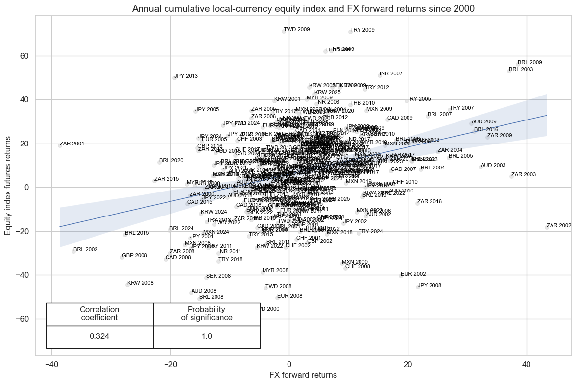
OLS regression reveals a highly significant positive intercept, implying that on average, the FX forward returns need to be quite negative to result in negative equity index futures.
cr.ols_table()
                            OLS Regression Results
==============================================================================
Dep. Variable:               EQXR_NSA   R-squared:                       0.105
Model:                            OLS   Adj. R-squared:                  0.103
Method:                 Least Squares   F-statistic:                     45.00
Date:                Thu, 25 Sep 2025   Prob (F-statistic):           7.08e-11
Time:                        17:43:14   Log-Likelihood:                -1696.8
No. Observations:                 386   AIC:                             3398.
Df Residuals:                     384   BIC:                             3405.
Df Model:                           1
Covariance Type:            nonrobust
==============================================================================
                 coef    std err          t      P>|t|      [0.025      0.975]
------------------------------------------------------------------------------
const          5.8848      1.005      5.856      0.000       3.909       7.861
FXXR_NSA       0.6199      0.092      6.708      0.000       0.438       0.802
==============================================================================
Omnibus:                       24.166   Durbin-Watson:                   2.248
Prob(Omnibus):                  0.000   Jarque-Bera (JB):               41.715
Skew:                          -0.404   Prob(JB):                     8.74e-10
Kurtosis:                       4.393   Cond. No.                         10.9
==============================================================================

Notes:
[1] Standard Errors assume that the covariance matrix of the errors is correctly specified.
Appendices #
Appendix 1: Equity index specification #
The following equity indices have been used for futures return calculations in each currency area:
-
AUD: Standard and Poor’s / Australian Stock Exchange 200
-
BRL: Brazil Bovespa
-
CAD: Standard and Poor’s / Toronto Stock Exchange 60 Index
-
CHF: Swiss Market (SMI)
-
CNY: Shanghai Shenzhen CSI 300
-
DEM: DAX 30 Performance (Xetra)
-
ESP: IBEX 35
-
EUR: EURO STOXX 50
-
FRF: CAC 40
-
GBP: FTSE 100
-
HKD: Hang Seng China Enterprises
-
INR: CNX Nifty (50)
-
ITL: FTSE MIB Index
-
JPY: Nikkei 225 Stock Average
-
KRW: Korea Stock Exchange KOSPI 200
-
MXN: Mexico IPC (Bolsa)
-
MYR: FTSE Bursa Malaysia KLCI
-
NLG: AEX Index (AEX)
-
PLN: Warsaw General Index 20
-
SEK: OMX Stockholm 30 (OMXS30)
-
SGD: MSCI Singapore (Free)
-
THB: Bangkok S.E.T. 50
-
TRY: Bist National 30
-
TWD: Taiwan Stock Exchange Weighed TAIEX
-
USD: Standard and Poor’s 500 Composite
-
ZAR: FTSE / JSE Top 40
See Appendix 3 for the list of currency symbols used to represent each cross-section.
Appendix 2: Alternative equity index specification #
Alternative equity indices are available for the following currency areas:
-
HKD: Hang Seng
-
JPY: TOPIX
-
USD: NASDAQ 100
-
USD: Russell 2000
See Appendix 3 for the list of currency symbols used to represent each cross-section.
Appendix 3: Currency symbols #
The word ‘cross-section’ refers to currencies, currency areas or economic areas. In alphabetical order, these are AUD (Australian dollar), BRL (Brazilian real), CAD (Canadian dollar), CHF (Swiss franc), CLP (Chilean peso), CNY (Chinese yuan renminbi), COP (Colombian peso), CZK (Czech Republic koruna), DEM (German mark), ESP (Spanish peseta), EUR (Euro), FRF (French franc), GBP (British pound), HKD (Hong Kong dollar), HUF (Hungarian forint), IDR (Indonesian rupiah), ITL (Italian lira), JPY (Japanese yen), KRW (Korean won), MXN (Mexican peso), MYR (Malaysian ringgit), NLG (Dutch guilder), NOK (Norwegian krone), NZD (New Zealand dollar), PEN (Peruvian sol), PHP (Phillipine peso), PLN (Polish zloty), RON (Romanian leu), RUB (Russian ruble), SEK (Swedish krona), SGD (Singaporean dollar), THB (Thai baht), TRY (Turkish lira), TWD (Taiwanese dollar), USD (U.S. dollar), ZAR (South African rand).