Labor market dynamics #
This category group contains real-time measures of changes in employment, employment and productivity. Whilst labor market dynamics are often seen as lagging indicators of business cycles, they are also indicative of the impact of the economic situation on private households, popular sentiment and labor cost.
Employment growth #
Ticker : EMPL_NSA_P1M1ML12 / _P1M1ML12_3MMA / _P1Q1QL4
Label : Employment growth: %oya / %oya, 3mma / %oya, quarterly
Definition : Main measure of employment growth: % over a year ago / % over a year ago, 3-month moving average / % over a year ago, quarterly
Notes :
-
Employment data is taken only from official statistics, not job agencies or surveys.
-
Most countries release monthly-frequency data with fairly short publication lags. However, the following currency areas only release quarterly data: Switzerland (CHF), Czech Republic (CZK), the Eurozone (EUR), Mexico (MXN), Norway (NOK), New Zealand (NZD), the Phillipines (PHP), Singapore (SGD), Thailand (THB) and South Africa (ZAR). There are no employment growth rates on a monthly frequency for these countries.
-
The UK (GBP) and Peru (PEN) only release employment in 3-month moving averages. However, these are updated at a monthly frequency.
-
Employment growth has not been calculated for countries and periods with semi-annual and annual data, most prominently China and Indonesia.
Unemployment growth #
Ticker : UNEMPLRATE_NSA_3MMA_D1M1ML12 / _D1Q1QL4
Label : Unemployment rate change: oya, 3mma / oya, quarterly
Definition : Change in unemployment rate: over a year ago, 3-month moving average / over a year ago, quarterly
Notes :
-
Unemployment data is taken only from official statistics, not job agencies or surveys.
-
Most countries release monthly-frequency data with fairly short publication lags. However, the following currency areas only release quarterly data: the Phillipines (PHP), Singapore (SGD) and South Africa (ZAR). There are no unemployment growth rates on a monthly frequency for these countries.
-
Brazil (BRL) and Peru (PEN) only release unemployment in 3-month moving averages. However, these are updated at a monthly frequency.
-
Unemployment growth has not been calculated for countries that only provide semi-annual and annual data, most prominently China and Indonesia.
Ticker : UNEMPLRATE_SA_D3M3ML3 / _D6M6ML6 / _D1Q1QL1 / _D2Q2QL2
Label : Unemployment growth, seasonally adjusted: difference 3 months over 3 months ago / difference 6 months over 6 months ago / difference 1 quarter over 1 quarter ago / difference 2 quarters over 2 quarters ago
Definition : Change in seasonally adjusted unemployment rate: 3 months over previous 3 months / 6 months over previous 6 months / quarter over previous quarter / 2 quarters over previous two quarters
Notes :
-
Unemployment data is taken only from official statistics, not job agencies or surveys.
-
Most countries release monthly-frequency data with fairly short publication lags. However, the following currency areas only release quarterly data: the Phillipines (PHP), Thailand (THB) and South Africa (ZAR). There are no unemployment growth rates on a monthly frequency for these countries.
-
Brazil (BRL), the UK (GBP) and Peru (PEN) only release seasonally adjusted unemployment in 3-month moving averages. However, these are updated at a monthly frequency.
-
Unemployment growth has not been calculated for countries and periods with semi-annual and annual data, most prominently China and Indonesia.
Labour productivity #
Ticker : RGDPPW_SA_P1Q1QL4 / _P1Qv2YMA / _P1Qv5YMA
Label : Real GDP (1-year moving average) per workforce, sa: % oya / % 1q vs 2yma / % 1q vs 5yma
Definition : Real GDP (1-year moving average) per workforce, seasonally adjusted: % over a year ago / % change, latest quarter versus 2-year moving average / % change, latest quarter versus 5-year moving average
Notes :
-
Work force data are taken from national statistics sources and the World Bank.
-
Due to workforce being a yearly series and significantly behind real GDP we estimate up to date and quarterly values by taking the 3 year difference of moving median for workforce and adding that to latest value and interpolating to get the quarterly values.
Ticker : RGDPPE_SA_P1Q1QL4 / _P1Qv2YMA / _P1Qv5YMA
Label : Real GDP (1-year moving average) per employee, sa: % oya / % 1q vs 2yma / % 1q vs 5yma
Definition : Real GDP (1-year moving average) per employee, seasonally adjusted: % over a year ago / % change, latest quarter versus 2-year moving average / % change, latest quarter versus 5-year moving average
Notes :
-
Employment data is taken only from official statistics, not job agencies or surveys.
-
Employment numbers used in calculation are also a one year moving average.
-
Due to CNY employment series being a yearly series the same procedure is done as the workforce ratios.
Ticker : MANUPE_SA_P1M1ML12 / _P1M1ML12_3MMA / _P1Mv2YMA / _P1Mv5YMA
Label : Maufacturing ouput (1-year moving average) per employee, sa: % oya / % oya, 3mma, / % 1m vs 2yma / % 1m vs 5yma
Definition : Manufacturing output (1-year moving average) per manufacturing employee, seasonally adjusted: % over a year ago / % over a year ago, 3 month moving average / % change, latest quarter versus 2-year moving average / % change, latest quarter versus 5-year moving average
Notes :
-
In this case employment figures are related to manufacturing employment.
-
We form a synthetic index by taking the one year moving average of manufacturing component of industrial production and then dividing it by manufacturing employees and finally working out the transformations.
-
Due to CNY and RUB manufacturing employment series being a yearly only series the same procedure is done as the workforce ratios.
-
As CNY only publishes growth figures for manufacturing output only percent over ago indicators are calculated.
-
CZK, IDR, ILS, INR, MYR, PEN do not publish manufacturing employee numbers and thus are not included.
Imports #
Only the standard Python data science packages and the specialized
macrosynergy
package are needed.
import os
import numpy as np
import pandas as pd
import matplotlib.pyplot as plt
import seaborn as sns

import macrosynergy.management as msm
import macrosynergy.panel as msp
import macrosynergy.signal as mss
import macrosynergy.pnl as msn
import macrosynergy.visuals as msv

from macrosynergy.download import JPMaQSDownload

import warnings
warnings.simplefilter("ignore")
The
JPMaQS
indicators we consider are downloaded using the J.P. Morgan Dataquery API interface within the
macrosynergy
package. This is done by specifying
ticker strings
, formed by appending an indicator category code
<category>
to a currency area code
<cross_section>
. These constitute the main part of a full quantamental indicator ticker, taking the form
DB(JPMAQS,<cross_section>_<category>,<info>)
, where
<info>
denotes the time series of information for the given cross-section and category.
The following types of information are available:
-
valuegiving the latest available values for the indicator -
eop_lagreferring to days elapsed since the end of the observation period -
mop_lagreferring to the number of days elapsed since the mean observation period -
gradedenoting a grade of the observation, giving a metric of real time information quality.
After instantiating the
JPMaQSDownload
class within the
macrosynergy.download
module, one can use the
            download(tickers,


            start_date,


            metrics)
method to obtain the data. Here
tickers
is an array of ticker strings,
start_date
is the first release date to be considered and
metrics
denotes the types of information requested.
# Cross-sections of interest

cids_dmca = [
    "AUD",
    "CAD",
    "CHF",
    "EUR",
    "GBP",
    "JPY",
    "NOK",
    "NZD",
    "SEK",
    "USD",
]  # DM currency areas
cids_dmec = ["DEM", "ESP", "FRF", "ITL", "NLG"]  # DM euro area countries
cids_latm = ["BRL", "COP", "CLP", "MXN", "PEN"]  # Latam countries
cids_emea = ["CZK", "HUF", "ILS", "PLN", "RON", "RUB", "TRY", "ZAR"]  # EMEA countries
cids_emas = [
    "CNY",
    "HKD",
    "IDR",
    "INR",
    "KRW",
    "MYR",
    "PHP",
    "SGD",
    "THB",
    "TWD",
]  # EM Asia countries

cids_dm = cids_dmca + cids_dmec
cids_em = cids_latm + cids_emea + cids_emas

# For Equity analysis:

cids_g3 = ["EUR", "JPY", "USD"]  # DM large currency areas
cids_dmes = ["AUD", "CAD", "CHF", "GBP", "SEK"]  # Smaller DM equity countries
cids_dmeq = cids_g3 + cids_dmes  # DM equity countries

# For FX analysis:
cids_nofx = ["USD", "EUR", "CNY", "SGD", "HKD"]
cids_dmfx = list(set(cids_dmca) - set(cids_nofx)) # DM currencies excluding USD, EUR
cids_emfx = list(set(cids_em) - set(cids_nofx))


cids = sorted(cids_dm + cids_em)
cids_lab = sorted(list(set(cids) - set(["CNY", "IDR", "INR"])))
cids_rgdppe = sorted(list(set(cids) - set(cids_dmec + ["HKD"])))
# Quantamental categories of interest

main = [
    "EMPL_NSA_P1M1ML12",
    "EMPL_NSA_P1M1ML12_3MMA",
    "EMPL_NSA_P1Q1QL4",
    "UNEMPLRATE_NSA_3MMA_D1M1ML12",
    "UNEMPLRATE_NSA_D1Q1QL4",
    "UNEMPLRATE_SA_D3M3ML3",
    "UNEMPLRATE_SA_D6M6ML6",
    "UNEMPLRATE_SA_D1Q1QL1",
    "UNEMPLRATE_SA_D2Q2QL2",
    "RGDPPW_SA_P1Q1QL4",
    "RGDPPW_SA_P1Qv2YMA",
    "RGDPPW_SA_P1Qv5YMA",
    "RGDPPE_SA_P1Q1QL4",
    "RGDPPE_SA_P1Qv2YMA",
    "RGDPPE_SA_P1Qv5YMA",
    "MANUPE_SA_P1M1ML12",
    "MANUPE_SA_P1M1ML12_3MMA",
    "MANUPE_SA_P1Mv5YMA",
    "MANUPE_SA_P1Mv2YMA",
]
econ = [
    "INTRGDP_NSA_P1M1ML12_3MMA",
    "IMPORTS_SA_P1M1ML12_3MMA",
    "UNEMPLRATE_SA_3MMA",
    "UNEMPLRATE_SA_3MMAv5YMA",
    "WFORCE_NSA_P1Y1YL1_5YMM",
    "WAGES_NSA_P1M1ML12",
    "WAGES_NSA_P1Q1QL4",
]  # economic context
mark = [
    "FXXR_NSA",
    "EQXR_NSA",
    "DU05YXR_NSA",
    "DU05YXR_VT10",
    "DU02YXR_NSA",
    "DU02YXR_VT10",
    "FXTARGETED_NSA",
    "FXUNTRADABLE_NSA",
    "DU10YXR_NSA",
    "FXXR_VT10",
    "FXXRHvGDRB_NSA"
]  # market links

xcats = main + econ + mark

cids_co = ["GLD"]  # gold
xcats_co = ["COXR_VT10", "COXR_NSA"]  # Commodity future returns

tix_co = [c + "_" + x for c in cids_co for x in xcats_co]  # gold futures returns
# Download series from J.P. Morgan DataQuery by tickers

tickers = [cid + "_" + xcat for cid in cids for xcat in xcats]
tickers = tickers + tix_co

print(f"Maximum number of tickers is {len(tickers)}")
start_date="2000-01-01"
end_date = (pd.Timestamp.today() - pd.offsets.BDay(1)).strftime('%Y-%m-%d')


# Retrieve credentials

client_id: str = os.getenv("DQ_CLIENT_ID")
client_secret: str = os.getenv("DQ_CLIENT_SECRET")

with JPMaQSDownload(client_id=client_id, client_secret=client_secret) as dq:
    df = dq.download(
        tickers=tickers,
     #   start_date=start_date,
        suppress_warning=True,
        metrics=["all"],
        show_progress=True,
    )

dfx = df
Maximum number of tickers is 1408
Downloading data from JPMaQS.
Timestamp UTC:  2025-05-06 08:54:07
Connection successful!
Requesting data: 100%|███████████████████████████████████████████████████████████████| 282/282 [00:59<00:00,  4.72it/s]
Downloading data: 100%|██████████████████████████████████████████████████████████████| 282/282 [04:44<00:00,  1.01s/it]
Some expressions are missing from the downloaded data. Check logger output for complete list.
1636 out of 5632 expressions are missing. To download the catalogue of all available expressions and filter the unavailable expressions, set `get_catalogue=True` in the call to `JPMaQSDownload.download()`.
Some dates are missing from the downloaded data.
2 out of 6614 dates are missing.
Availability #
cids_exp = cids_lab  # cids expected in category panels
msm.missing_in_df(df, xcats=main[0:9], cids=cids_exp)
No missing XCATs across DataFrame.
Missing cids for EMPL_NSA_P1M1ML12:             ['CHF', 'CZK', 'EUR', 'FRF', 'GBP', 'MXN', 'NLG', 'NOK', 'NZD', 'PEN', 'PHP', 'SGD', 'THB', 'ZAR']
Missing cids for EMPL_NSA_P1M1ML12_3MMA:        ['CHF', 'CZK', 'EUR', 'FRF', 'MXN', 'NLG', 'NOK', 'NZD', 'PHP', 'SGD', 'THB', 'ZAR']
Missing cids for EMPL_NSA_P1Q1QL4:              ['AUD', 'BRL', 'CAD', 'CLP', 'COP', 'DEM', 'ESP', 'GBP', 'HKD', 'HUF', 'ILS', 'ITL', 'JPY', 'KRW', 'MYR', 'PEN', 'PLN', 'RON', 'RUB', 'SEK', 'TRY', 'TWD', 'USD']
Missing cids for UNEMPLRATE_NSA_3MMA_D1M1ML12:  ['ESP', 'NZD', 'PHP', 'SGD', 'ZAR']
Missing cids for UNEMPLRATE_NSA_D1Q1QL4:        ['AUD', 'BRL', 'CAD', 'CHF', 'CLP', 'COP', 'CZK', 'DEM', 'ESP', 'EUR', 'FRF', 'GBP', 'HKD', 'HUF', 'ILS', 'ITL', 'JPY', 'KRW', 'MXN', 'MYR', 'NLG', 'NOK', 'PEN', 'PLN', 'RON', 'RUB', 'SEK', 'THB', 'TRY', 'TWD', 'USD']
Missing cids for UNEMPLRATE_SA_D1Q1QL1:         ['AUD', 'BRL', 'CAD', 'CHF', 'CLP', 'COP', 'CZK', 'DEM', 'EUR', 'FRF', 'GBP', 'HKD', 'HUF', 'ILS', 'ITL', 'JPY', 'KRW', 'MXN', 'MYR', 'NLG', 'NOK', 'NZD', 'PEN', 'PLN', 'RON', 'RUB', 'SEK', 'SGD', 'TRY', 'TWD', 'USD']
Missing cids for UNEMPLRATE_SA_D2Q2QL2:         ['AUD', 'BRL', 'CAD', 'CHF', 'CLP', 'COP', 'CZK', 'DEM', 'EUR', 'FRF', 'GBP', 'HKD', 'HUF', 'ILS', 'ITL', 'JPY', 'KRW', 'MXN', 'MYR', 'NLG', 'NOK', 'NZD', 'PEN', 'PLN', 'RON', 'RUB', 'SEK', 'SGD', 'TRY', 'TWD', 'USD']
Missing cids for UNEMPLRATE_SA_D3M3ML3:         ['ESP', 'PHP', 'THB', 'ZAR']
Missing cids for UNEMPLRATE_SA_D6M6ML6:         ['ESP', 'PHP', 'THB', 'ZAR']
Availability of real-time quantamental indicators of labor market dynamics, either quarterly or monthly, is very diverse, with some series’ going back to the 1970s and others only starting in the 2010s.
For the explanation of currency symbols, which are related to currency areas or countries for which categories are available, please view Appendix 1 .
xcatx = main[0:9]
cidx = cids_lab

msm.check_availability(
    df,
    xcats=xcatx,
    cids=cidx,
    missing_recent=False,
)

Vintage grading is mixed, with Chile the only country with high grade vintages consistently available across indicators.
xcatx = main[0:9]
cidx = cids_lab

plot = msp.heatmap_grades(
    df,
    xcats=xcatx,
    cids=cidx,
    start=start_date,
    size=(16, 4),
    title=f"Average vintage grades, from {start_date} onwards",
)

xcatx = ["EMPL_NSA_P1M1ML12", "EMPL_NSA_P1M1ML12_3MMA", "EMPL_NSA_P1Q1QL4"]
cidx = cids_lab
msp.view_ranges(
    df,
    xcats=xcatx,
    cids=cidx,
    val="eop_lag",
    title="End of observation period lags (ranges of time elapsed since end of observation period in days)",
    start="2000-01-01",
    kind="box",
    size=(16, 4),
)
msp.view_ranges(
    df,
    xcats=xcatx,
    cids=cidx,
    val="mop_lag",
    title="Median of observation period lags (ranges of time elapsed since middle of observation period in days)",
    start="2000-01-01",
    kind="box",
    size=(16, 4),
)


xcatx = [
    "UNEMPLRATE_SA_D3M3ML3",
    "UNEMPLRATE_SA_D6M6ML6",
    "UNEMPLRATE_SA_D1Q1QL1",
    "UNEMPLRATE_SA_D2Q2QL2",
]
cidx = cids_lab
msp.view_ranges(
    df,
    xcats=xcatx,
    cids=cidx,
    val="eop_lag",
    title="End of observation period lags (ranges of time elapsed since end of observation period in days)",
    start="2000-01-01",
    kind="box",
    size=(16, 4),
)
msp.view_ranges(
    df,
    xcats=xcatx,
    cids= cidx,
    val="mop_lag",
    title="Median of observation period lags (ranges of time elapsed since middle of observation period in days)",
    start="2000-01-01",
    kind="box",
    size=(16, 4),
)


cids_exp = cids_rgdppe  # cids expected in category panels
msm.missing_in_df(df, xcats=main[10:], cids=cids_rgdppe)
No missing XCATs across DataFrame.
Missing cids for MANUPE_SA_P1M1ML12:       ['CZK', 'IDR', 'ILS', 'INR', 'MYR', 'PEN']
Missing cids for MANUPE_SA_P1M1ML12_3MMA:  ['CZK', 'IDR', 'ILS', 'INR', 'MYR', 'PEN']
Missing cids for MANUPE_SA_P1Mv2YMA:       ['CNY', 'CZK', 'IDR', 'ILS', 'INR', 'MYR', 'PEN']
Missing cids for MANUPE_SA_P1Mv5YMA:       ['CNY', 'CZK', 'IDR', 'ILS', 'INR', 'MYR', 'PEN']
Missing cids for RGDPPE_SA_P1Q1QL4:        ['INR']
Missing cids for RGDPPE_SA_P1Qv2YMA:       ['INR']
Missing cids for RGDPPE_SA_P1Qv5YMA:       ['INR']
Missing cids for RGDPPW_SA_P1Qv2YMA:       []
Missing cids for RGDPPW_SA_P1Qv5YMA:       []
Most real GDP ratios are available since 2000, while the manufacturing output per employee is much more diverse and generally later.
xcatx = main[9:]
cidx = cids_rgdppe

msm.check_availability(
    df,
    xcats=xcatx,
    cids=cidx,
    missing_recent=False,
)

Vintage grading is mixed, with developed countries have high grade vintages compared to developing countries.
xcatx = main[9:]
cidx = cids_rgdppe

plot = msp.heatmap_grades(
    df,
    xcats=xcatx,
    cids=cidx,
    start=start_date,
    size=(16, 4),
    title=f"Average vintage grades, from {start_date} onwards",
)

For the purpose of the below presentation, we have renamed quarterly-frequency indicators to approximate monthly equivalents in order to have a full panel of similar measures across most countries. The two series’ are not identical but are close substitutes.
olds = [

    "EMPL_NSA_P1Q1QL4", "UNEMPLRATE_NSA_D1Q1QL4", "WAGES_NSA_P1Q1QL4"
]
news = [

    "EMPL_NSA_P1M1ML12_3MMA","UNEMPLRATE_NSA_3MMA_D1M1ML12","WAGES_NSA_P1M1ML12"
]


dfx = df.replace(to_replace=olds, value=news)

scols = ["cid", "xcat", "real_date", "value"]
dfx = dfx[scols].copy().sort_values(["cid", "xcat", "real_date"])
dfx["ticker"] = dfx["cid"] + "_" + dfx["xcat"]
History #
Employment growth #
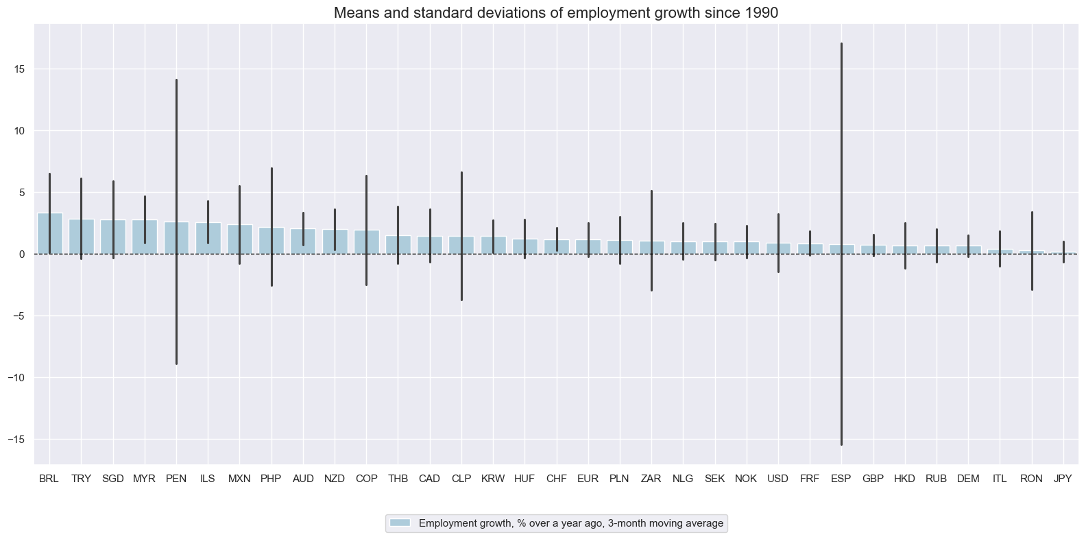
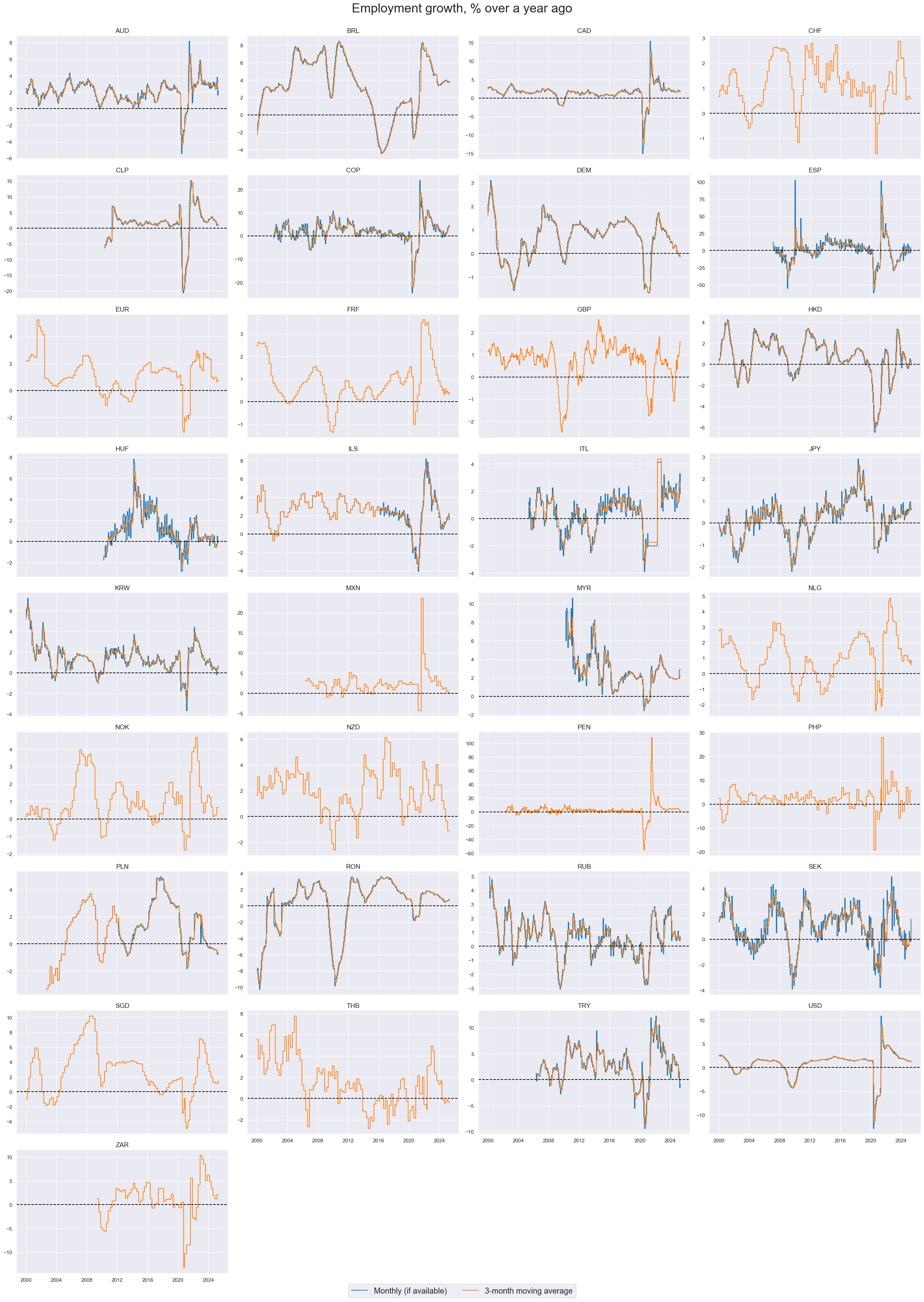
Employment growth has been positive across all currency areas since 2000 or over the available sample periods. Fluctuations have been larger in American economies than elsewhere.
cidx = list(set(cids_lab) - set(["TWD", "CZK"]))
xcatx = ["EMPL_NSA_P1M1ML12_3MMA"]

msp.view_ranges(
    dfx,
    xcats=xcatx,
    cids=cidx,
    sort_cids_by="mean",
    start=start_date,
    kind="bar",
    size=(16, 8),
    title="Means and standard deviations of employment growth since 1990",
    xcat_labels=["Employment growth, % over a year ago, 3-month moving average"],
)
cidx = sorted(list(set(cids_lab) - set(["TWD", "CZK"])))
xcatx = ["EMPL_NSA_P1M1ML12", "EMPL_NSA_P1M1ML12_3MMA"]

msp.view_timelines(
    dfx,
    xcats=xcatx,
    cids=cidx,
    start=start_date,
    title="Employment growth, % over a year ago",
    xcat_labels=["Monthly (if available)", "3-month moving average"],
    ncol=4,
    same_y=False,
    legend_fontsize=17,
    title_fontsize=27,
    size=(12, 7),
    all_xticks=False,
)
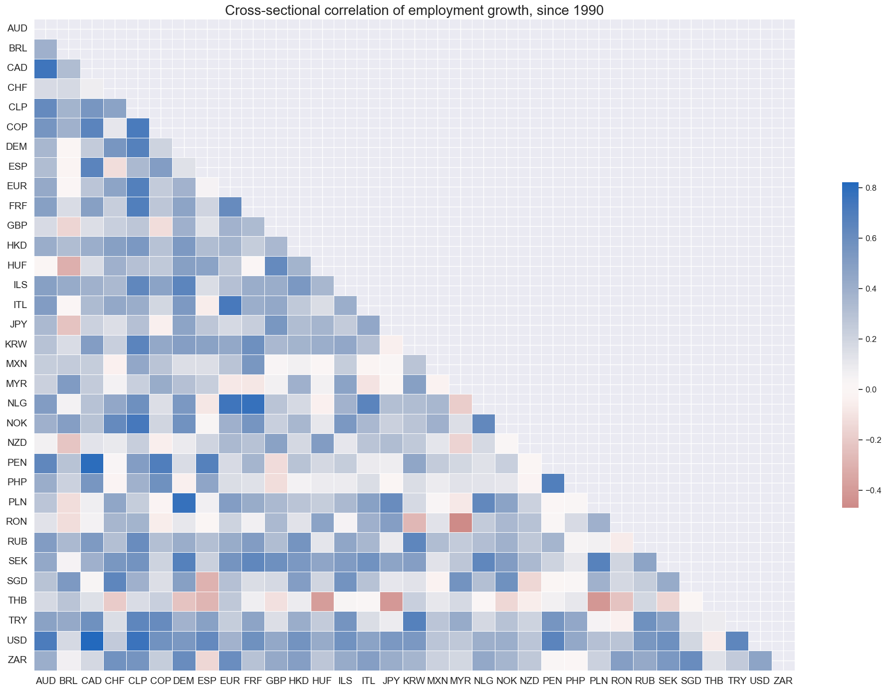
Information states of employment growth has been predominantly positively correlated across currency markets. All countries, except for Thailand, have displayed positive correlation with U.S. payroll growth.
msp.correl_matrix(
    dfx,
    xcats="EMPL_NSA_P1M1ML12_3MMA",
    cids=cidx,
    size=(20, 14),
    start=start_date,
    title="Cross-sectional correlation of employment growth, since 1990",
)
Annual changes in unemployment rates #
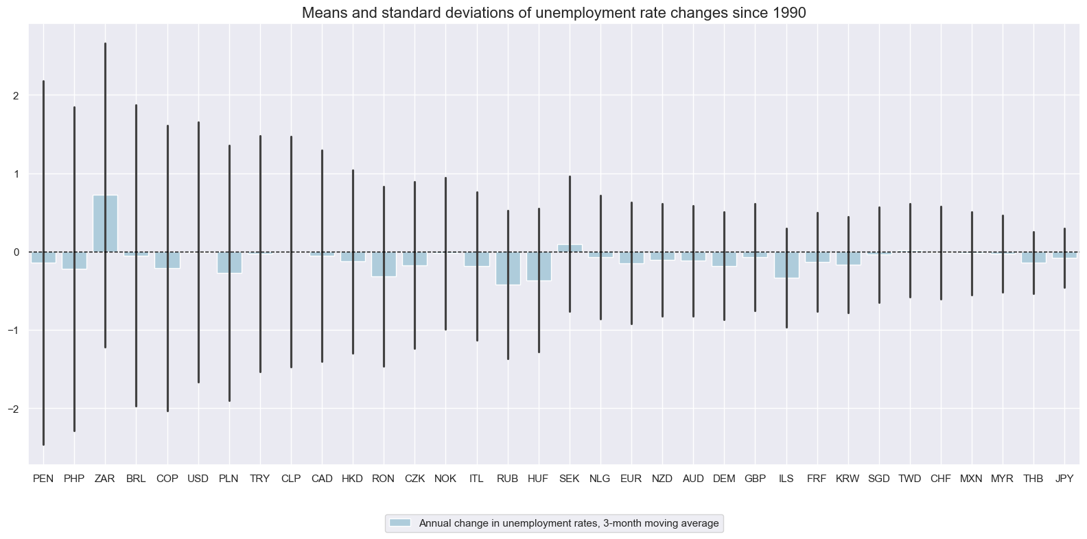
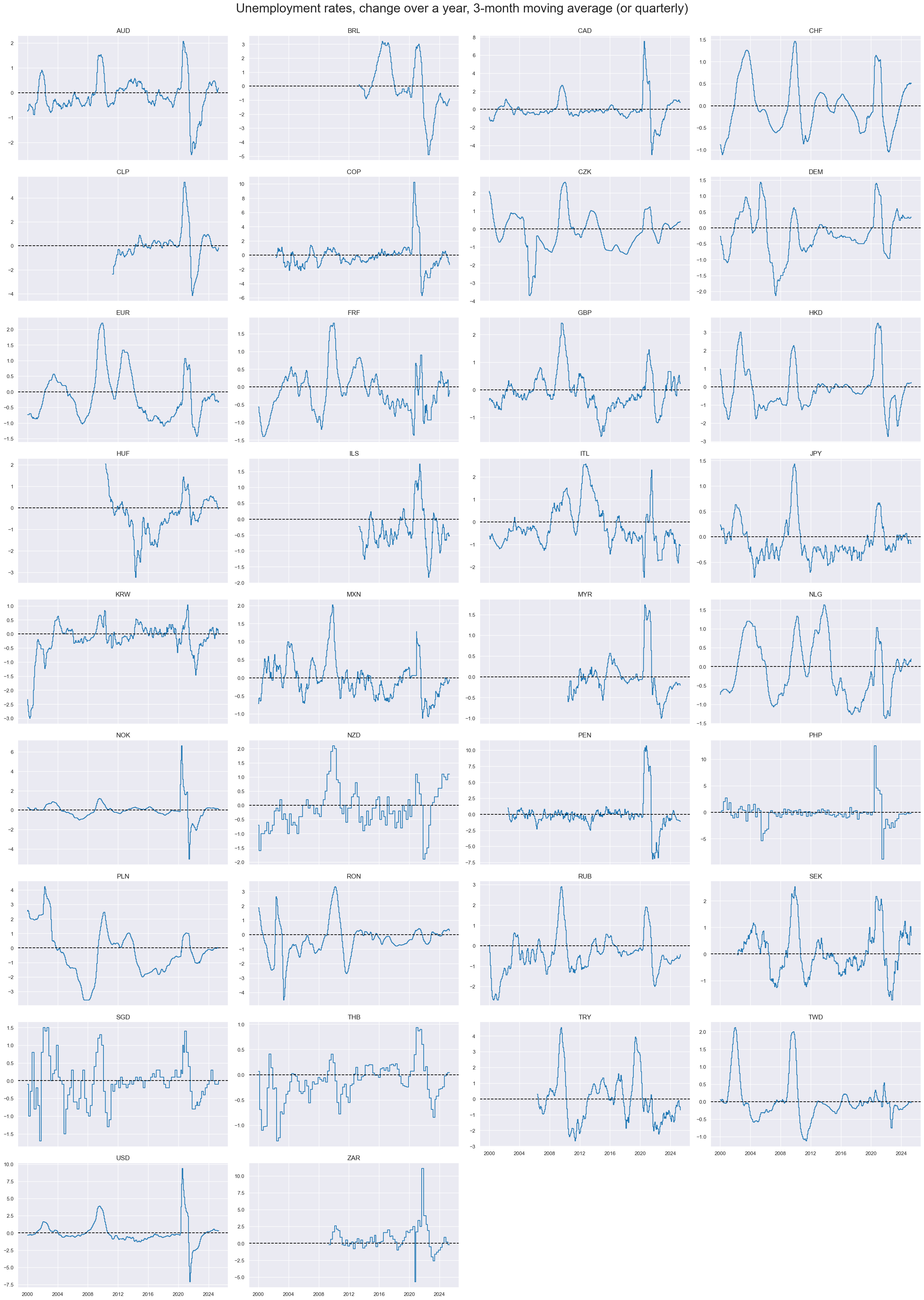
Volatility of unemployment rate changes have been very different across countries, reflecting differences in labor markets and social security incentives for registration, as well as the general registered level of joblessness.
xcatx = ["UNEMPLRATE_NSA_3MMA_D1M1ML12"]
cidx = list(set(cids_lab))

msp.view_ranges(
    dfx,
    xcats=xcatx,
    cids=cidx,
    sort_cids_by="std",
    start=start_date,
    title="Means and standard deviations of unemployment rate changes since 1990",
    xcat_labels=["Annual change in unemployment rates, 3-month moving average"],
    kind="bar",
    size=(16, 8),
)
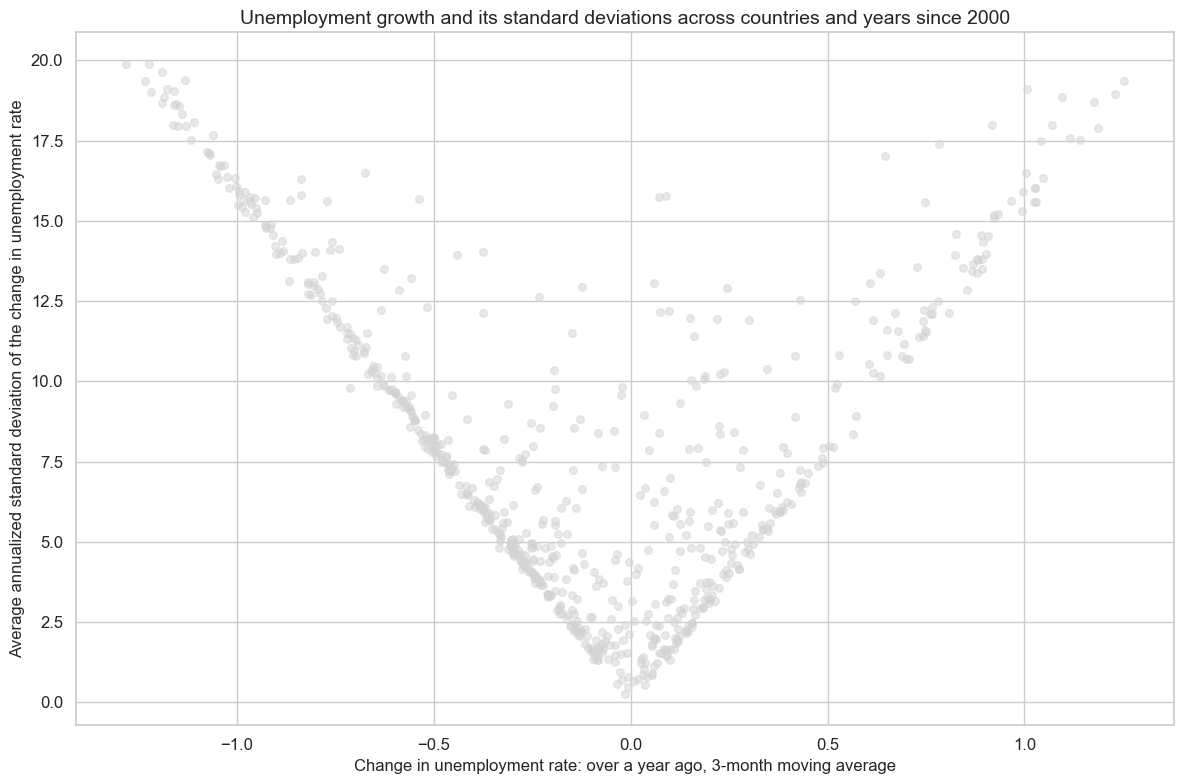
Similar to demographic trend indicators, there has been a clear linear relation between average unemployment growth and its standard deviation, across currency areas and years. This suggests high absolute unemployment growth comes with high uncertainty. This inherent uncertainty leads to more pronounced fluctuations in unemployment rates, resulting in a higher standard deviation.
dfa = msp.historic_vol(
    dfx, xcat="UNEMPLRATE_NSA_3MMA_D1M1ML12", cids=cids, lback_meth="xma", postfix="_ASD"
)
dfx = msm.update_df(dfx, dfa)


cr = msp.CategoryRelations(
    dfx,
    xcats=["UNEMPLRATE_NSA_3MMA_D1M1ML12", "UNEMPLRATE_NSA_3MMA_D1M1ML12_ASD"],
    cids=cids_lab,
    freq="A",
    lag=0,
    xcat_aggs=["mean", "mean"],
    xcat_trims=[20, 20],
    start="2000-01-01",
)

cr.reg_scatter(
    title="Unemployment growth and its standard deviations across countries and years since 2000",
    xlab="Change in unemployment rate: over a year ago, 3-month moving average",
    ylab="Average annualized standard deviation of the change in unemployment rate",
    prob_est="map",
    fit_reg=False,
    coef_box=None,
    )
UNEMPLRATE_NSA_3MMA_D1M1ML12 misses: ['ESP'].
UNEMPLRATE_NSA_3MMA_D1M1ML12_ASD misses: ['ESP'].
xcatx = ["UNEMPLRATE_NSA_3MMA_D1M1ML12"]
cidx = sorted(list(set(cids_lab)))

msp.view_timelines(
    dfx,
    xcats=xcatx,
    cids=cidx,
    start=start_date,
    title="Unemployment rates, change over a year, 3-month moving average (or quarterly)",
    legend_fontsize=17,
    title_fontsize=27,
    xcat_labels=["3-month moving average"],
    ncol=4,
    same_y=False,
    size=(12, 7),
    all_xticks=False,
)
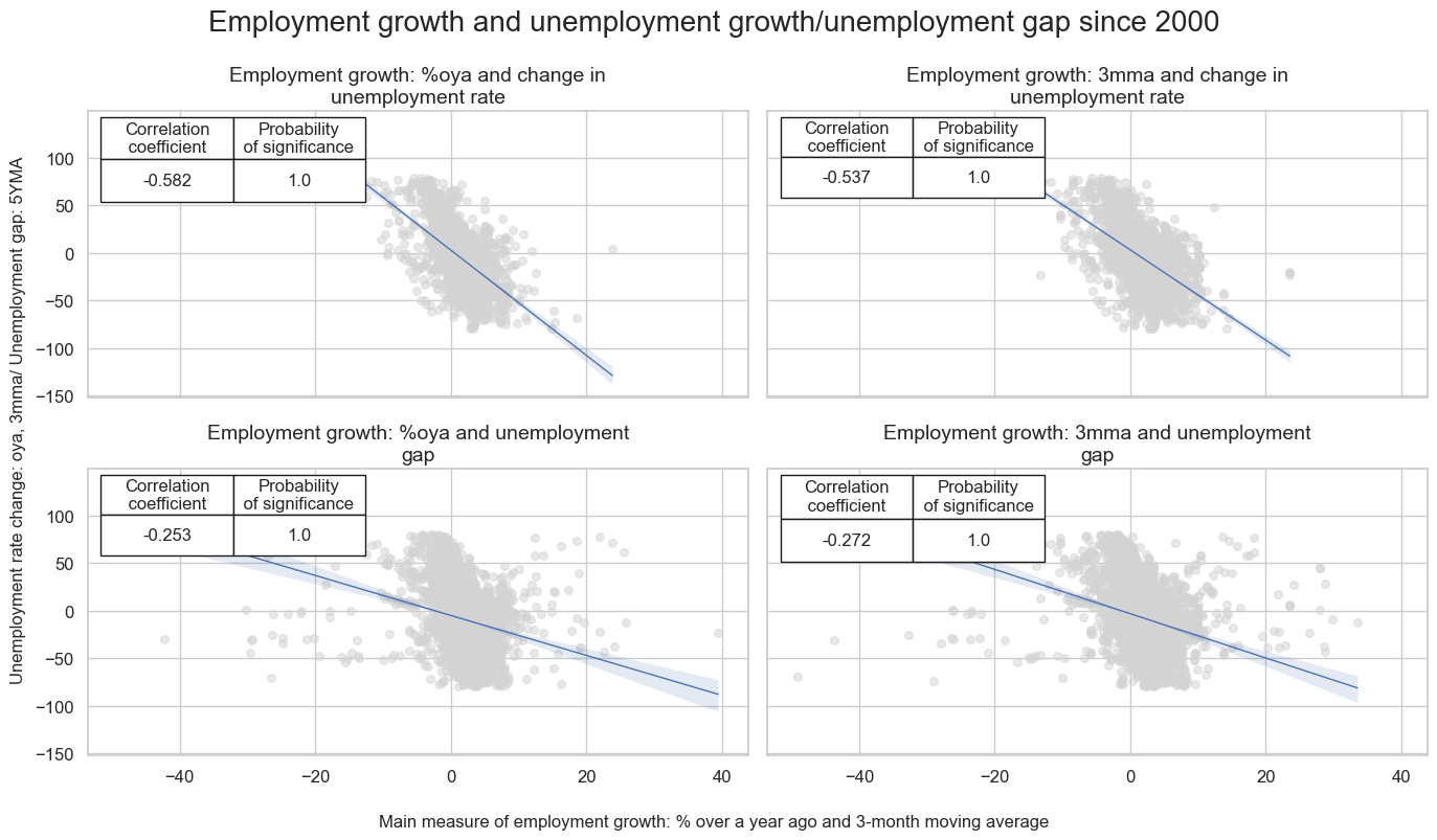
Employment growth is strongly, but not perfectly (negatively) correlated with the change in unemployment rate, reflecting the different methodologies of the two metrics as well as the influence of labor participation rates. Using monthly averages, the magnitude of negative correlation has been roughly 60%. Scatterplots reveal a number of outliers.
The same relationship holds for employment growth and unemployment gap, labor market tightness indicator.
easy_labels = {
    "EMPL_NSA_P1M1ML12": "Employment growth: %oya",
    "EMPL_NSA_P1M1ML12_3MMA": "Employment growth: 3mma",
   }


cr_empl= {}
cr_emplgap= {}

empl=["EMPL_NSA_P1M1ML12", "EMPL_NSA_P1M1ML12_3MMA"]

for sig in empl:
    cr_empl[f"cr_{sig}"] = msp.CategoryRelations(
        dfx,
        xcats=[sig, "UNEMPLRATE_NSA_3MMA_D1M1ML12"],
        cids=cids_lab,
        freq="M",
        lag=1,
        xcat_aggs=["last", "sum"],
        start=start_date,
        xcat_trims=[80, 80]
    )

for sig in empl:
    cr_emplgap[f"cr_{sig}"] = msp.CategoryRelations(
        dfx,
        xcats=[sig, "UNEMPLRATE_SA_3MMAv5YMA"],
        cids=cids_lab,
        freq="M",
        lag=1,
        xcat_aggs=["last", "sum"],
        start=start_date,
        xcat_trims=[50, 80]
    )

msv.multiple_reg_scatter(
    cat_rels = [cr_empl["cr_"+ key] for key in list(easy_labels.keys())]+[cr_emplgap["cr_"+ key] for key in list(easy_labels.keys())],
    title="Employment growth and unemployment growth/unemployment gap since 2000",
    xlab="Main measure of employment growth: % over a year ago and 3-month moving average",
    ylab="Unemployment rate change: oya, 3mma/ Unemployment gap: 5YMA",
    figsize=(14, 8),
    ncol=2,
    nrow=2,
    prob_est="map",
    coef_box="upper left",
    subplot_titles = [f"{lab} and change in unemployment rate" for lab in easy_labels.values()] + \
                 [f"{lab} and unemployment gap" for lab in easy_labels.values()]
)
EMPL_NSA_P1M1ML12 misses: ['CHF', 'CZK', 'EUR', 'FRF', 'GBP', 'MXN', 'NLG', 'NOK', 'NZD', 'PEN', 'PHP', 'SGD', 'THB', 'ZAR'].
UNEMPLRATE_NSA_3MMA_D1M1ML12 misses: ['ESP'].
UNEMPLRATE_NSA_3MMA_D1M1ML12 misses: ['ESP'].
EMPL_NSA_P1M1ML12 misses: ['CHF', 'CZK', 'EUR', 'FRF', 'GBP', 'MXN', 'NLG', 'NOK', 'NZD', 'PEN', 'PHP', 'SGD', 'THB', 'ZAR'].
Shorter-term changes in unemployment rates #
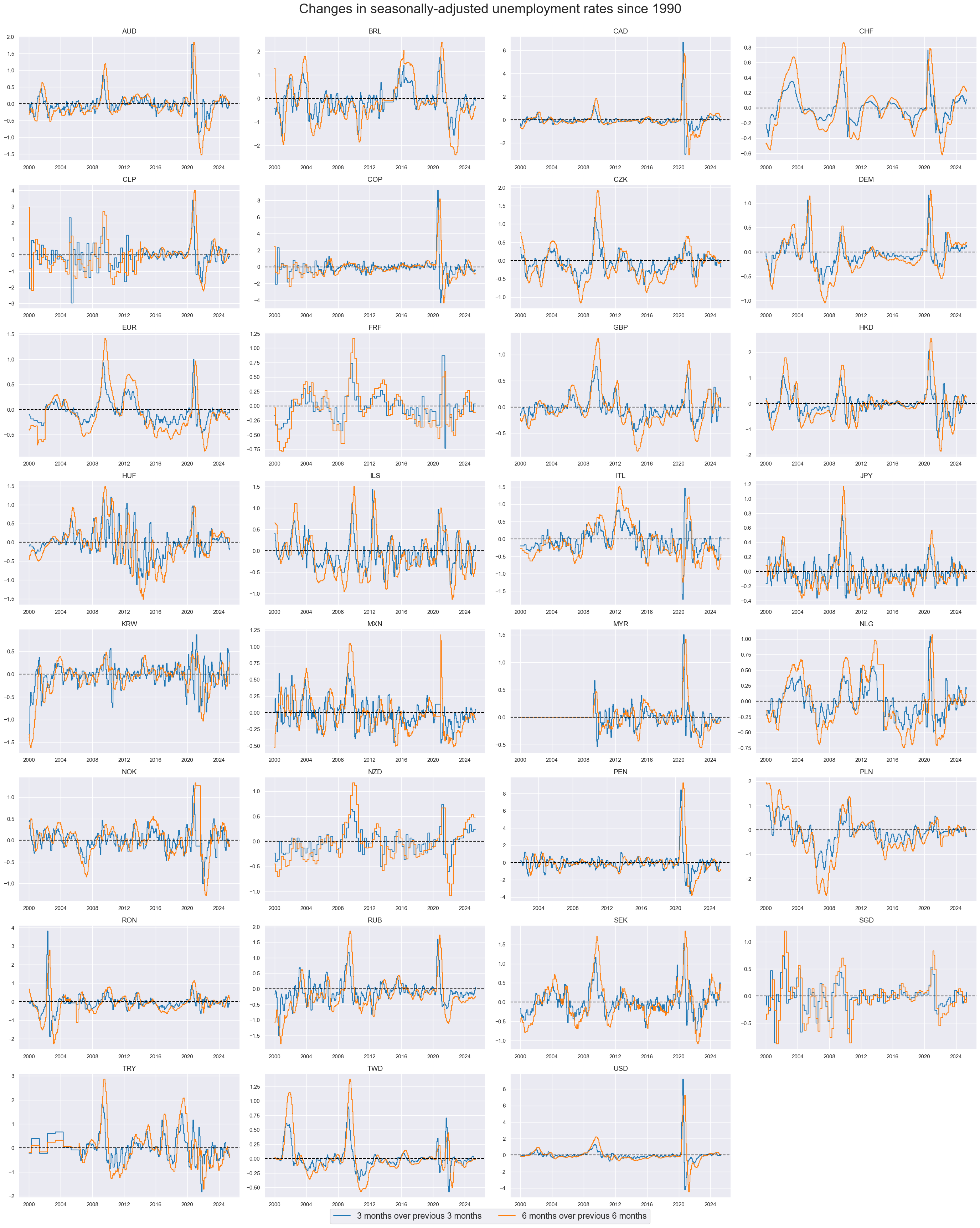
Seasonally adjusted unemployment changes can be more timely in detecting labor market and broader business cycle trends.
The 6-month-over-6-month changes look like good trend indicators for most countries. The 3-month-over-3-month changes are subject to greater volatility, but often detect large shifts in labor market conditions earlier.
xcatx = ["UNEMPLRATE_SA_D3M3ML3", "UNEMPLRATE_SA_D6M6ML6"]
cidx = cids_lab
msp.view_timelines(
    dfx,
    xcats=xcatx,
    cids=cidx,
    start=start_date,
    title="Changes in seasonally-adjusted unemployment rates since 1990",
    xcat_labels=["3 months over previous 3 months", "6 months over previous 6 months"],
    legend_fontsize=17,
    title_fontsize=27,
    ncol=4,
    same_y=False,
    size=(12, 7),
    all_xticks=True,
)
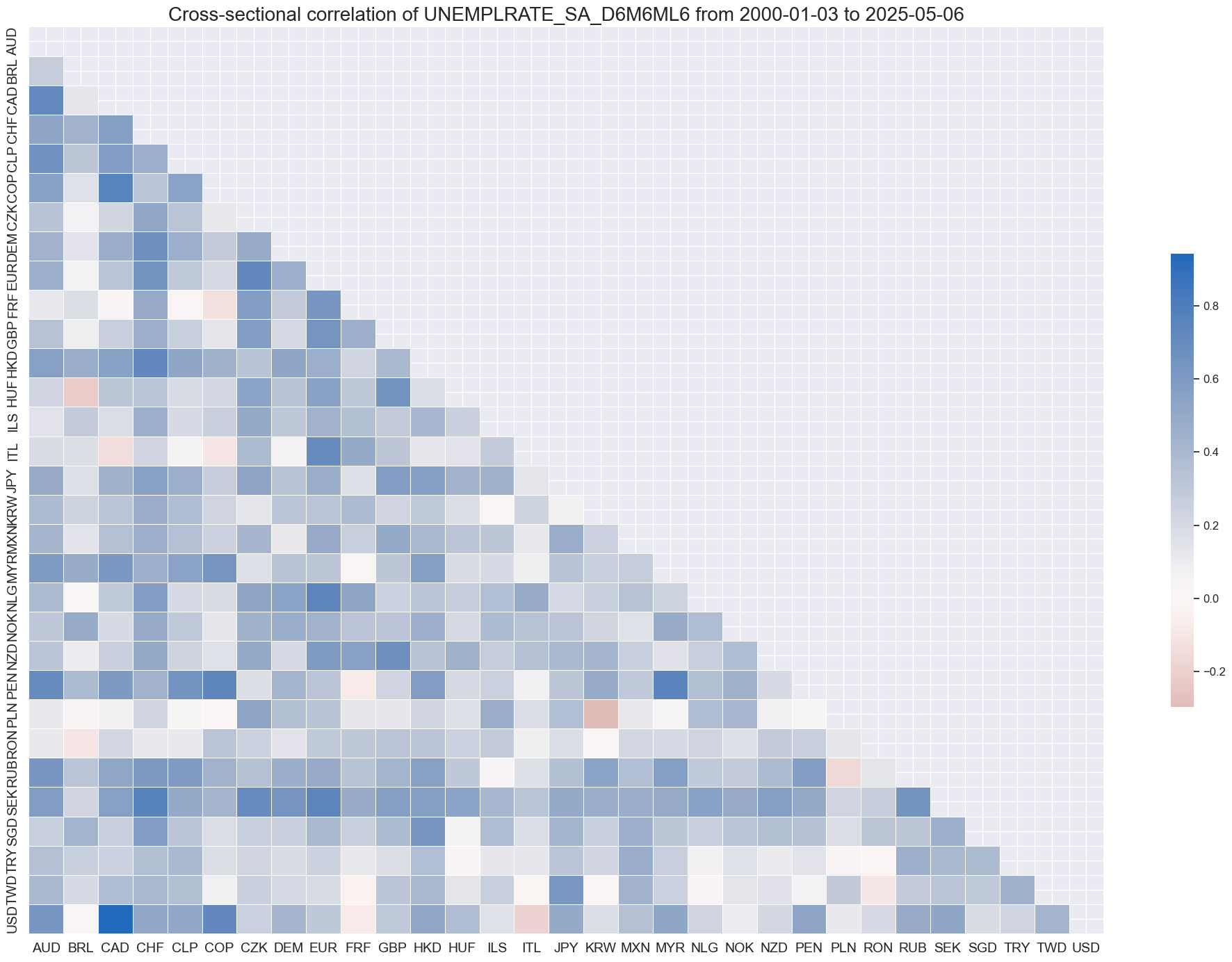
Information states on unemployment trends have been dominantly positively correlated across currency markets.
msp.correl_matrix(dfx,
                  xcats="UNEMPLRATE_SA_D6M6ML6",
                  cids=cidx,
                  size=(20, 14))
Labour productivity #
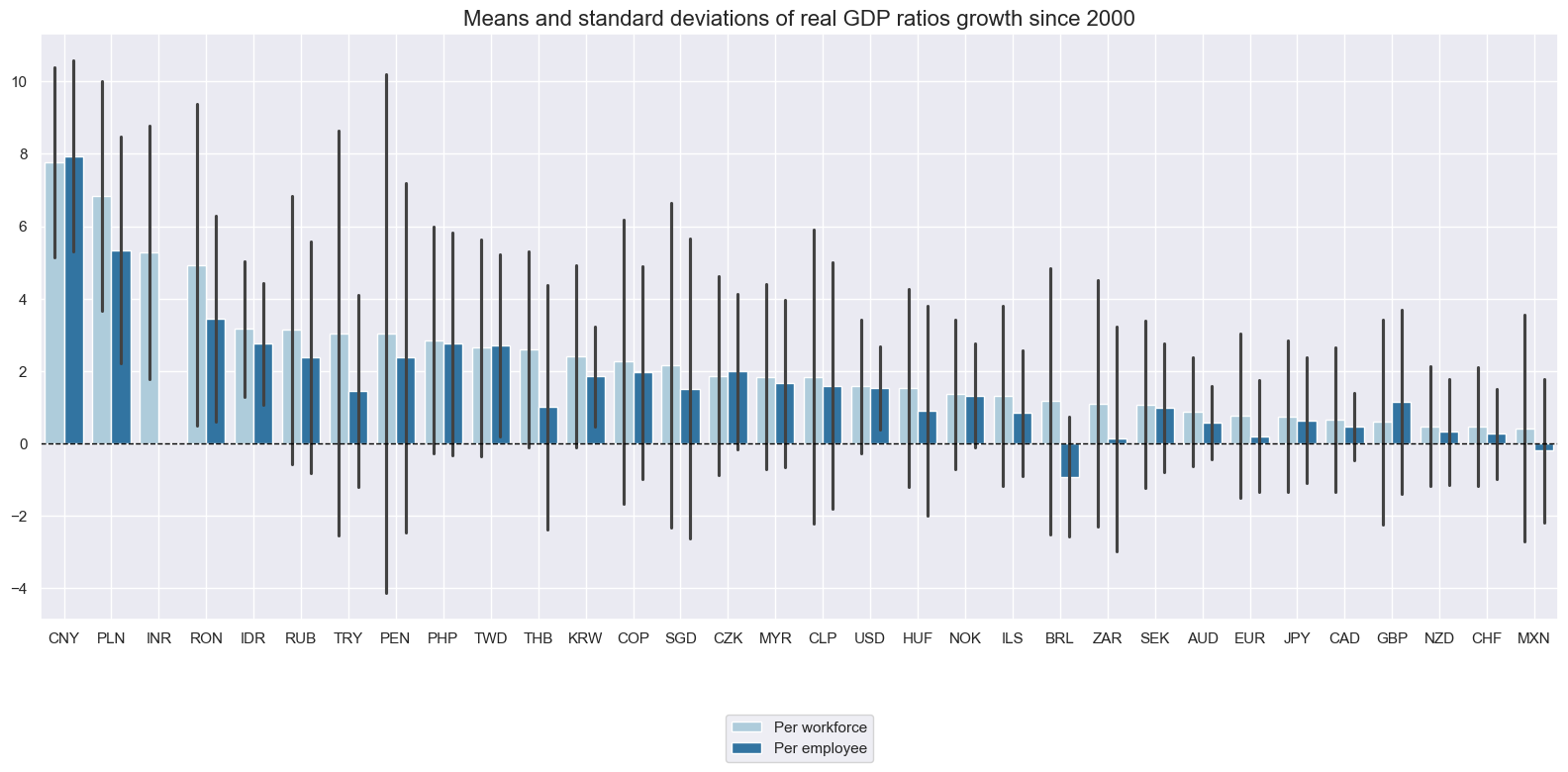
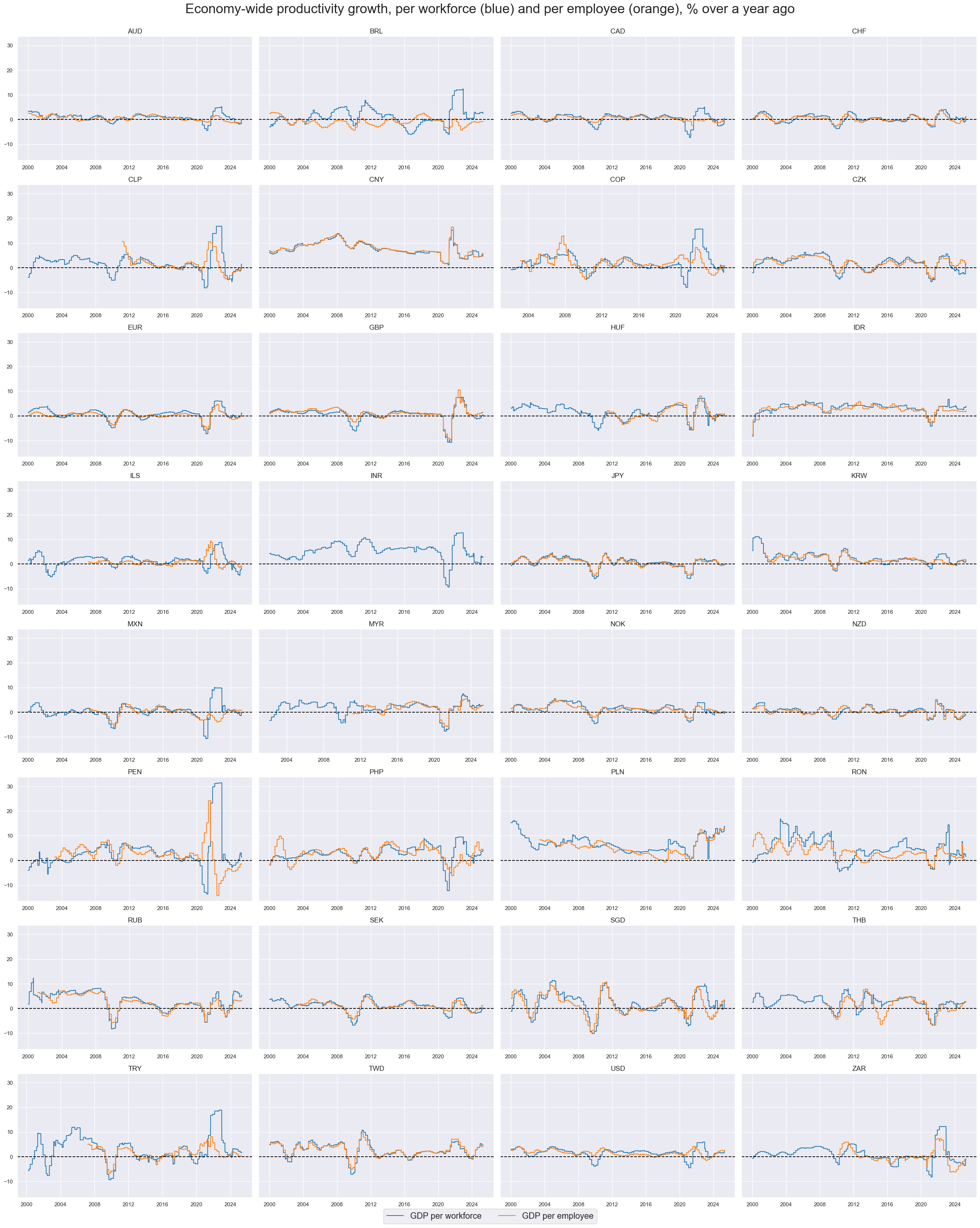
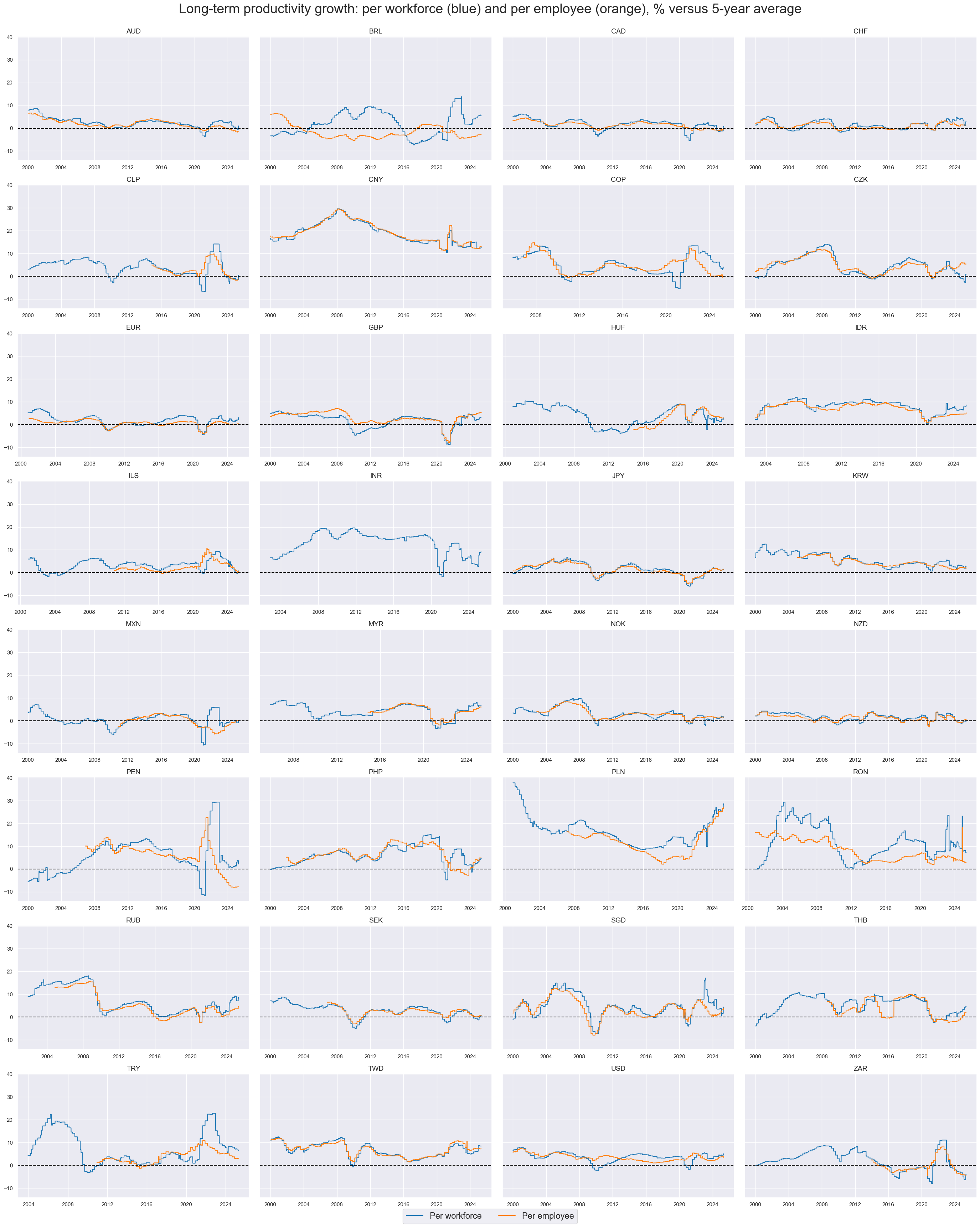
Long-term means and standard deviations of economy-wide labor productivity growth have been quite diverse across countries. Output growth per workforce has outpaced output growth per employee most countries, with the notable exception of China and the UK.
cidx = list(set(cids_rgdppe))
xcatx = ["RGDPPW_SA_P1Q1QL4","RGDPPE_SA_P1Q1QL4"]

msp.view_ranges(
    dfx,
    xcats=xcatx,
    cids=cidx,
    sort_cids_by="mean",
    start=start_date,
    kind="bar",
    size=(16, 8),
    title="Means and standard deviations of real GDP ratios growth since 2000",
    xcat_labels=["Per workforce", "Per employee"],
)
xcatx = ["RGDPPW_SA_P1Q1QL4","RGDPPE_SA_P1Q1QL4"]
cidx = sorted(list(set(cids_rgdppe)))
msp.view_timelines(
    dfx,
    xcats=xcatx,
    cids=cidx,
    start=start_date,
    title="Economy-wide productivity growth, per workforce (blue) and per employee (orange), % over a year ago",
    xcat_labels=["GDP per workforce", "GDP per employee"],
    legend_fontsize=17,
    title_fontsize=27,
    ncol=4,
    same_y=True,
    size=(12, 7),
    all_xticks=True,
)
xcatx = ["RGDPPW_SA_P1Qv5YMA","RGDPPE_SA_P1Qv5YMA"]
cidx = sorted(list(set(cids_rgdppe)))
msp.view_timelines(
    dfx,
    xcats=xcatx,
    cids=cidx,
    start=start_date,
    title="Long-term productivity growth: per workforce (blue) and per employee (orange), % versus 5-year average",
    xcat_labels=["Per workforce", "Per employee"],
    legend_fontsize=17,
    title_fontsize=27,
    ncol=4,
    same_y=True,
    size=(12, 7),
    all_xticks=True,
)
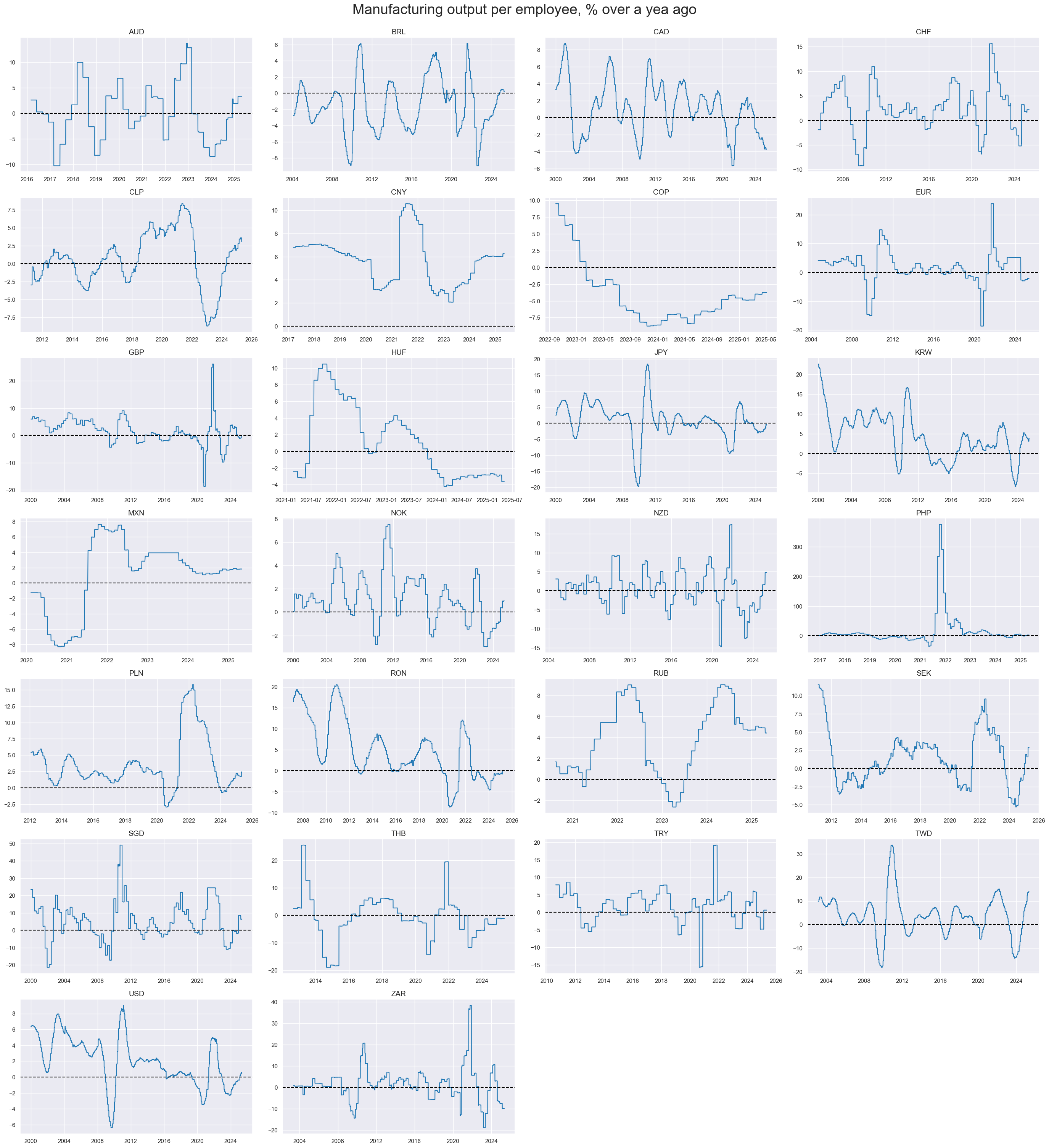
Manufacturing output appears to be highly cyclical.
xcatx = ["MANUPE_SA_P1M1ML12"]
cidx = sorted(list(set(cids_rgdppe)))
msp.view_timelines(
    dfx,
    xcats=xcatx,
    cids=cidx,
    start=start_date,
    title="Manufacturing output per employee, % over a yea ago",
    xcat_labels=None,
    legend_fontsize=17,
    title_fontsize=27,
    ncol=4,
    same_y=False,
    size=(12, 7),
    all_xticks=True,
)
Importance #
Research links #
On employment and bond prices:
“Interest rates have reacted strongly to the monthly employment report in recent years…The reaction of rates to the report and provide evidence that it has been stronger since the mid-1980s than in earlier years. Evidently the report now has greater impact…on expectations of where the Fed is going to move the federal funds rate. These expectations influence longer-term money market rates.” Cook and Korn
“The impact of an idiosyncratic rise in unemployment on bond yields turns out to be positive for European countries while it is negative for the United States and Australia. The speed of the response also varies.” Dimpfl and Langen
On unemployment and stock prices:
“…on average, the stock market responds positively to news of rising unemployment in expansions, and negatively in contractions. It follows that, since the economy is usually in an expansion phase, the stock market usually rises on bad labor market news.” John H. Boyd at al.
On unemployment and currency markets:
“… the findings indicate significant information spillovers across the labour and currency markets in both directions.” Deven Bathia at al.
“The analysis of the currency portfolios showed that on average, currencies associated with low growth of the unemployment rate offer higher returns than currencies associated with high growth of the unemployment rate. We found that typically the former appreciate and the latter depreciate” Federico Nucera
On employment and gold prices:
“The release of the U.S. jobs report has a considerable impact on gold spot exchange rates, the study’s findings show. According to the analysis, a high number of nonfarm payrolls has the most bearing on the announcement, while the unemployment rate and the revision from the previous month also add to the picture. It has been discovered that an upbeat job report weakens gold spot exchange rates. Additionally, the research has demonstrated that abnormal returns occur immediately following the announcement, indicating that the market is responding fast to the fresh information. The study’s decision tree methods, such as logistic regression and XGboost, have shown great precision and accuracy in forecasting the direction of gold spot exchange rates depending on the timing of the release of the U.S. employment report. Nima Niyazpour and Kaya Tokmakcioglu
Labor market dynamics indicators are used, for example, in the following Macrosynergy posts:
Empirical clues #
Employment growth and equity returns #
Employment growth has been strongly and negatively correlated with subsequent equity market performance in past decades. This plausibly reflects that strong labor market dynamics place upward pressure on real interest rates and wage growth. The relationship has prevailed across decades.
Simple employment growth is a powerful economic indicator on its own. However, it can be enhanced as detailed in the notebook Demographic trends , which involves adjusting the employment growth indicator by the workforce growth. This adjusted indicator shows a stronger correlation and significance with subsequent equity returns.
calcs = [
    "XEMPL_NSA_P1M1ML12_3MMA = EMPL_NSA_P1M1ML12_3MMA - WFORCE_NSA_P1Y1YL1_5YMM",
]

dfa = msp.panel_calculator(dfx, calcs=calcs, cids=cids_dm, blacklist=None)
dfx = msm.update_df(dfx, dfa)
dfxx = dfx[dfx["xcat"] == "EMPL_NSA_P1M1ML12_3MMA"]
dfxt = dfxx.pivot(index="real_date", columns="cid", values="value")
dfat = dfxt.sub(
    dfxt.median(axis=0), axis=1
)  # excess employment growth through median subtraction
dfa = dfat.unstack().reset_index().rename({0: "value"}, axis="columns")
dfa["xcat"] = "XEMPL_NSA_P1M1ML12_3MMA"
dfx = msm.update_df(dfx, dfa)
xcatx = ["EMPL_NSA_P1M1ML12_3MMA", "XEMPL_NSA_P1M1ML12_3MMA"]

easy_labels = {
    "EMPL_NSA_P1M1ML12_3MMA": "Employment growth trend",
    "XEMPL_NSA_P1M1ML12_3MMA": "Excess employment growth trend",
}

cr_equity = {}

for sig in xcatx:
    cr_equity[f"cr_{sig}"] = msp.CategoryRelations(
        dfx,
        xcats=[sig, "EQXR_NSA"],
        cids=cids_dmeq,
        freq="Q",
        lag=1,
        xcat_aggs=["last", "sum"],
        start=start_date,
        xcat_trims=[None, None],
    )


msv.multiple_reg_scatter(
    cat_rels=[cr_equity["cr_" + key] for key in list(easy_labels.keys())],
    title="Employment growth trends and subsequent equity returns, panel of 8 developed markets, since 2000",
    ylab="Next quarter's equity index future return, %",
    ncol=2,
    nrow=1,
    figsize=(20, 10),
    prob_est="map",
    coef_box="lower left",
    subplot_titles=[lab for lab in list(easy_labels.values())],
)
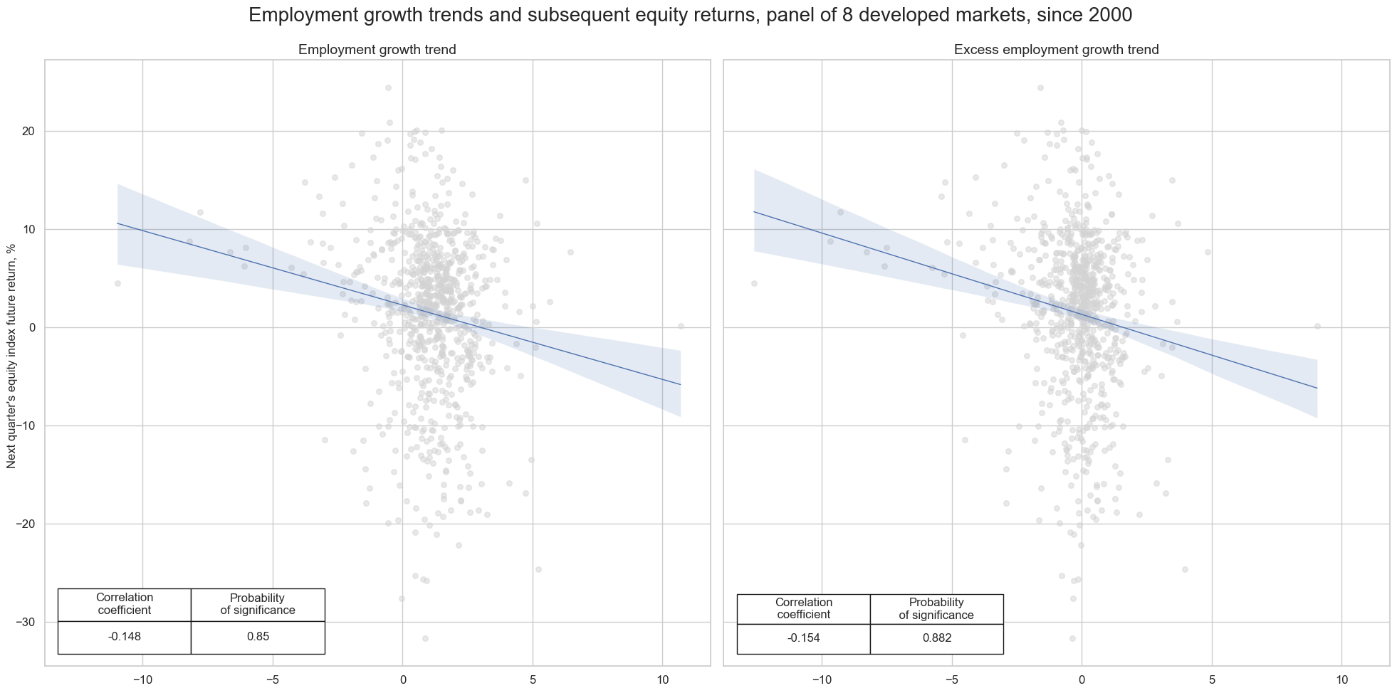
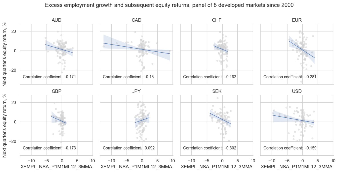
The negative correlation between employment growth (or excess employment growth) is consistent across almost all developed markets, apart from Japan, where the relationship is positive.
cr_equity["cr_XEMPL_NSA_P1M1ML12_3MMA"].reg_scatter(
    labels=False,
    coef_box="upper left",
    title="Excess employment growth and subsequent equity returns, panel of 8 developed markets since 2000",
    ylab="Next quarter's equity return, %",
    separator="cids",
  )
Employment growth versus FX benchmarks #
dfb = dfx[dfx["xcat"].isin(["FXTARGETED_NSA", "FXUNTRADABLE_NSA"])].loc[
    :, ["cid", "xcat", "real_date", "value"]
]
dfba = (
    dfb.groupby(["cid", "real_date"])
    .aggregate(value=pd.NamedAgg(column="value", aggfunc="max"))
    .reset_index()
)
dfba["xcat"] = "FXBLACK"
fxblack = msp.make_blacklist(dfba, "FXBLACK")
fxblack
{'BRL': (Timestamp('2012-12-03 00:00:00'), Timestamp('2013-09-30 00:00:00')),
 'CHF': (Timestamp('2011-10-03 00:00:00'), Timestamp('2015-01-30 00:00:00')),
 'CNY': (Timestamp('2000-01-03 00:00:00'), Timestamp('2025-05-05 00:00:00')),
 'CZK': (Timestamp('2014-01-01 00:00:00'), Timestamp('2017-07-31 00:00:00')),
 'HKD': (Timestamp('2000-01-03 00:00:00'), Timestamp('2025-05-05 00:00:00')),
 'ILS': (Timestamp('2000-01-03 00:00:00'), Timestamp('2005-12-30 00:00:00')),
 'INR': (Timestamp('2000-01-03 00:00:00'), Timestamp('2004-12-31 00:00:00')),
 'MYR_1': (Timestamp('2000-01-03 00:00:00'), Timestamp('2007-11-30 00:00:00')),
 'MYR_2': (Timestamp('2018-07-02 00:00:00'), Timestamp('2025-05-05 00:00:00')),
 'PEN': (Timestamp('2021-07-01 00:00:00'), Timestamp('2021-07-30 00:00:00')),
 'RON': (Timestamp('2000-01-03 00:00:00'), Timestamp('2005-11-30 00:00:00')),
 'RUB_1': (Timestamp('2000-01-03 00:00:00'), Timestamp('2005-11-30 00:00:00')),
 'RUB_2': (Timestamp('2022-02-01 00:00:00'), Timestamp('2025-05-05 00:00:00')),
 'SGD': (Timestamp('2000-01-03 00:00:00'), Timestamp('2025-05-05 00:00:00')),
 'THB': (Timestamp('2007-01-01 00:00:00'), Timestamp('2008-11-28 00:00:00')),
 'TRY_1': (Timestamp('2000-01-03 00:00:00'), Timestamp('2003-09-30 00:00:00')),
 'TRY_2': (Timestamp('2020-01-01 00:00:00'), Timestamp('2024-07-31 00:00:00'))}
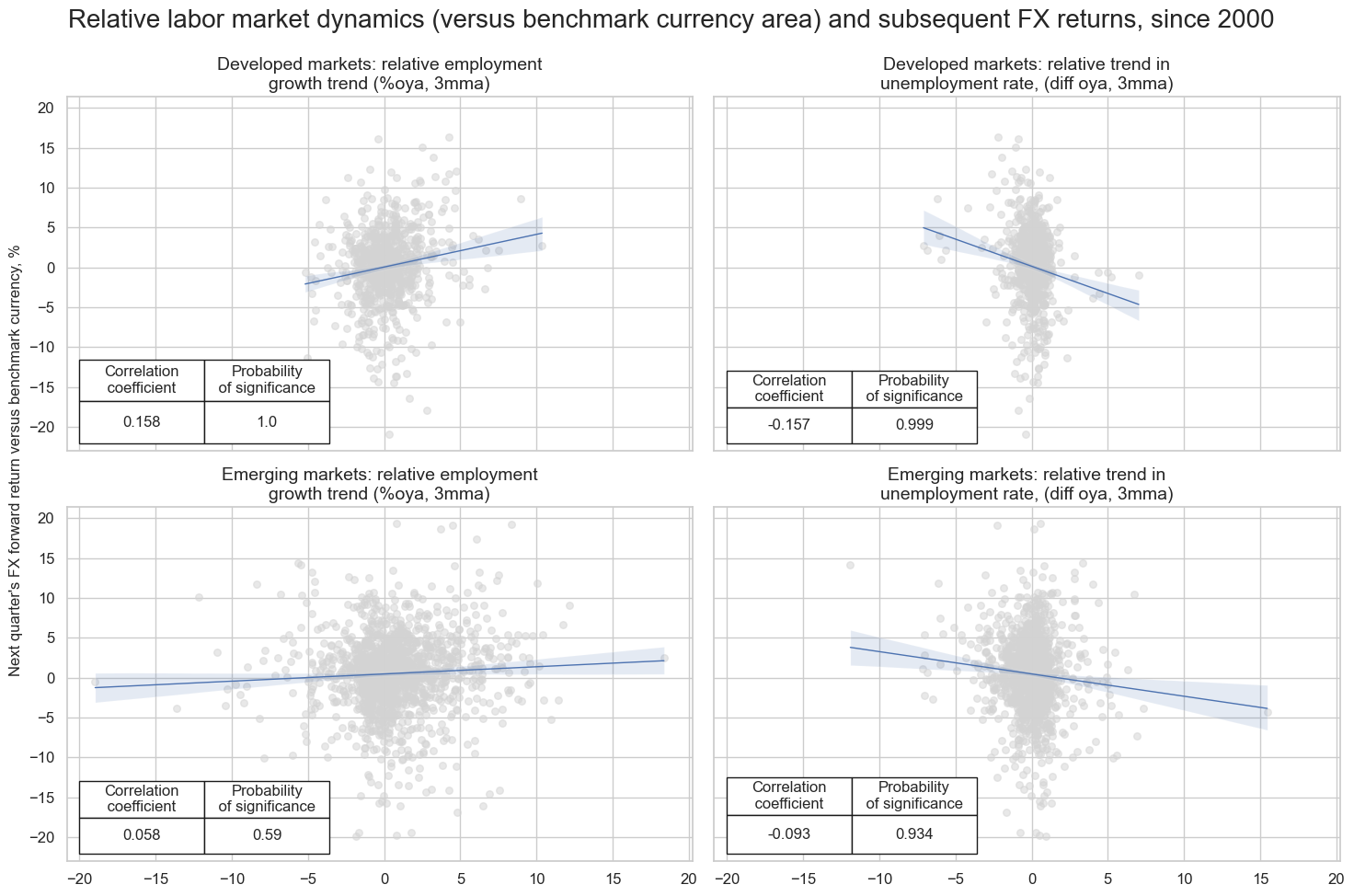
To explore the relationship between labor market dynamics indicators and subsequent FX returns, we calculate relative employment growth as the difference between quantamental indicators of reported employment trends in the reference currency area and the natural benchmark country. The growth trends are measured as % over a year ago in 3-month moving averages. In line with other posts, we calculate differentials to benchmarks for three types of currencies: those trading against USD, EUR and both USD and EUR. The list of currencies is as follows:
-
Currencies traded against EUR: [“CHF”, “CZK”, “HUF”, “NOK”, “PLN”, “RON”, “SEK”]
-
Currencies traded against USD and EUR: [“GBP”, “RUB”, “TRY”]. The benchmark equally weighs USD and EUR data
-
Currencies traded against USD: all other currencies
The new relative indicators receive postfix
_vBM
cids_fx = list(set(cids) - set(["EUR", "USD"]))
cids_eur = ["CHF", "CZK", "HUF", "NOK", "PLN", "RON", "SEK"]  # trading against EUR
cids_eud = ["GBP", "RUB", "TRY"]  # trading against EUR and USD
cids_usd = list(set(cids_fx) - set(cids_eur + cids_eud))  # trading against USD


xcatx = ["EMPL_NSA_P1M1ML12_3MMA", "XEMPL_NSA_P1M1ML12_3MMA", "UNEMPLRATE_NSA_3MMA_D1M1ML12"]

for xc in xcatx:
    calc_eur = [f"{xc}vBM = {xc} - iEUR_{xc}"]
    calc_usd = [f"{xc}vBM = {xc} - iUSD_{xc}"]
    calc_eud = [f"{xc}vBM = {xc} - 0.5 * ( iEUR_{xc} + iUSD_{xc} )"]

    dfa_eur = msp.panel_calculator(
        dfx,
        calcs=calc_eur,
        cids=cids_eur,
    )
    dfa_usd = msp.panel_calculator(
        dfx,
        calcs=calc_usd,
        cids=cids_usd,
    )
    dfa_eud = msp.panel_calculator(
        dfx,
        calcs=calc_eud,
        cids=cids_eud,
    )

    dfa = pd.concat([dfa_eur, dfa_usd, dfa_eud])
    dfx = msm.update_df(dfx, dfa)
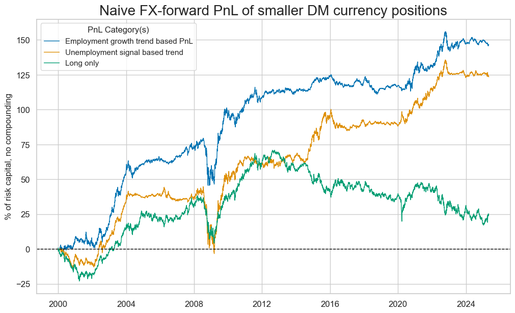
There is strong evidence of a positive predictive relation between relative labor market dynanmics, defined as relative improvement of the base currency area versus the benchmark (USD or EUR) and subsequent FX forward returns. We observe significant positive correlation between relative employment growth and subsequent fx returns in the next quarter for developed markets since 2000. For emerging markets, this relationship is also positive , but not quite significant, due probably to the lower quality and importance of payroll data in many EM countries. For both emerging and developed markets the relationship between relative unemployment trend and subsequent fx return has been negative and significant.
easyfx_labels = {
    "EMPL_NSA_P1M1ML12_3MMAvBM": "relative employment growth trend (%oya, 3mma)",
    "UNEMPLRATE_NSA_3MMA_D1M1ML12vBM": "relative trend in unemployment rate, (diff oya, 3mma)",
}

xcatx = ["EMPL_NSA_P1M1ML12_3MMAvBM", "UNEMPLRATE_NSA_3MMA_D1M1ML12vBM"]


cr_emfx = {}
cr_dmfx = {}

for sig in xcatx:
    cr_dmfx[f"cr_{sig}"] = msp.CategoryRelations(
        dfx,
        xcats=[sig, "FXXR_NSA"],
        cids=cids_dmfx,
        freq="Q",
        lag=1,
        xcat_aggs=["last", "sum"],
        blacklist=fxblack,
        start=start_date,
        xcat_trims=[None, None],
    )


for sig in xcatx:
    cr_emfx[f"cr_{sig}"] = msp.CategoryRelations(
        dfx,
        xcats=[sig, "FXXR_NSA"],
        cids=cids_emfx,
        freq="Q",
        lag=1,
        xcat_aggs=["last", "sum"],
        blacklist=fxblack,
        start=start_date,
        xcat_trims=[20, 20],
    )


msv.multiple_reg_scatter(
    cat_rels=[cr_dmfx["cr_" + key] for key in list(easyfx_labels.keys())]
    + [cr_emfx["cr_" + key] for key in list(easyfx_labels.keys())],
    title="Relative labor market dynamics (versus benchmark currency area) and subsequent FX returns, since 2000",
    ylab="Next quarter's FX forward return versus benchmark currency, %",
    ncol=2,
    nrow=2,
    figsize=(15, 10),
    prob_est="map",
    coef_box="lower left",
    subplot_titles=[f"Developed markets: {lab}" for lab in list(easyfx_labels.values())]
    + [f"Emerging markets: {lab}" for lab in list(easyfx_labels.values())],
)
EMPL_NSA_P1M1ML12_3MMAvBM misses: ['IDR', 'INR'].
UNEMPLRATE_NSA_3MMA_D1M1ML12vBM misses: ['IDR', 'INR'].
To check how well the labor market dynamics signals are predicting returns, we calculate accuracy measures, such as the share of correctly predicted directions of subsequent returns relative to all predictions. It not only shows an important aspect of feature-target co-movement but also implicitly tests if the signal’s neutral (zero) level has been well chosen. A particularly important metric for macro trading strategies is balanced accuracy, which is the average of the proportions of correctly predicted positive and negative returns. The robustness of accuracy metrics, parametric (Pearson) correlation, and non-parametric (Kendall) correlation should be checked across time periods, cross-sections, and variations of features and returns.
# Negative values

xcatx = ["EMPL_NSA_P1M1ML12_3MMA", "EMPL_NSA_P1M1ML12_3MMAvBM"]
calcs = []

for xc in xcatx:
    calcs += [f"{xc}_NEG = - {xc}"]

dfa = msp.panel_calculator(dfx, calcs=calcs, cids=cids_dmfx)
dfx = msm.update_df(dfx, dfa)

srr = mss.SignalReturnRelations(
    dfx,
    cids=cids_dmfx,
    sigs=["EMPL_NSA_P1M1ML12_3MMAvBM_NEG", "UNEMPLRATE_NSA_3MMA_D1M1ML12vBM"],
    blacklist=fxblack,
    sig_neg=[True, True] ,
    rets="FXXR_NSA",
    freqs=["M", "Q"],
    start=start_date,
)


tbx = (
    srr.multiple_relations_table(signal_name_dict={
        "EMPL_NSA_P1M1ML12_3MMAvBM_NEG_NEG": "Negative relative employment growth signal",
         "UNEMPLRATE_NSA_3MMA_D1M1ML12vBM_NEG": "Relative unemployment trend signal"},

         )
    .reset_index(level=["Aggregation", "Return", ], drop=True)
    .reset_index()
)

#tbx.set_index(["Signal", "Frequency"], inplace=True)

# for column modifications
dict_cols = {
    "Signal" : "Signal",
    "Frequency": "Frequency",
    "accuracy": "Accuracy",
    "bal_accuracy": "Balanced accuracy",
    "pos_sigr": "Share of positive signals",
    "pos_retr": "Share of positive returns",
    "pearson": "Pearson coefficient",
    "kendall": "Kendall coefficient",
}

# Filter and rename the columns

tbx = tbx[list(dict_cols.keys())]
tbx.rename(columns=dict_cols, inplace=True)
tbx.set_index(["Signal", "Frequency"], inplace=True)

tbx = tbx.style.format("{:.2f}").set_caption(
        "Predictive accuracy and correlation with respect to subsequent FXXR_NSA").set_table_styles(
       [{"selector": "caption", "props": [("text-align", "center"), ("font-weight", "bold"), ("font-size", "17px")]}])

display(tbx)
| Accuracy | Balanced accuracy | Share of positive signals | Share of positive returns | Pearson coefficient | Kendall coefficient | ||
|---|---|---|---|---|---|---|---|
| Signal | Frequency | ||||||
| Negative relative employment growth signal | M | 0.52 | 0.52 | 0.49 | 0.51 | 0.11 | 0.06 |
| Q | 0.53 | 0.53 | 0.49 | 0.52 | 0.16 | 0.08 | |
| Relative unemployment trend signal | M | 0.53 | 0.53 | 0.42 | 0.52 | 0.09 | 0.06 |
| Q | 0.54 | 0.55 | 0.42 | 0.53 | 0.16 | 0.09 |
naive_pnl = msn.NaivePnL(
    dfx,
    ret="FXXR_NSA",
    sigs=["EMPL_NSA_P1M1ML12_3MMAvBM_NEG", "UNEMPLRATE_NSA_3MMA_D1M1ML12vBM"],
    cids=cids_dmfx,
    start="2000-01-01",

)

for sig in ["EMPL_NSA_P1M1ML12_3MMAvBM_NEG", "UNEMPLRATE_NSA_3MMA_D1M1ML12vBM"]:
    naive_pnl.make_pnl(
        sig,
        sig_neg=True,
        sig_op="zn_score_pan",
        thresh=2,
        rebal_freq="monthly",
        vol_scale=10,
        rebal_slip=1,
        pnl_name=sig + "_PZN",
    )

naive_pnl.make_long_pnl(vol_scale=10, label="Long")
Naive PnL for both employment growth signal and for unemployment trend signal display consistent outperformance in relation of FX-forward position:
naive_pnl.plot_pnls(
    pnl_cats=naive_pnl.pnl_names,
    pnl_cids=["ALL"],
    title="Naive FX-forward PnL of smaller DM currency positions",
    xcat_labels={
    "EMPL_NSA_P1M1ML12_3MMAvBM_NEG_PZN": "Employment growth trend based PnL",
    "UNEMPLRATE_NSA_3MMA_D1M1ML12vBM_PZN": "Unemployment signal based trend",
    "Long": "Long only"}
    )
USD excess employment growth versus gold returns #
We compile a separate dataframe containing US labor market dynamics, including previously calculated excess employment trends and gold futures returns. For future calculations, we assign the ticker
"GLD"
to this US series.
# Pick the commodity returns

filt_cat = dfx["xcat"].isin(["COXR_VT10", "COXR_NSA"])
filt_cid = dfx["cid"].isin(["GLD"])
dfx_gld = dfx[filt_cat & filt_cid]

# Pick the U.S. indicators and assign them to the gold cross-section


xcatx = main + ["XEMPL_NSA_P1M1ML12_3MMA", "XUNEMPLRATE_SA_D6M6ML6"]
filt_cat = dfx["xcat"].isin(xcatx)
filt_cid = dfx["cid"] == "USD"

dfx_usd = dfx[filt_cat & filt_cid]
dfx_usd["cid"] = "GLD"
dfx_gld = msm.update_df(dfx_gld, dfx_usd)
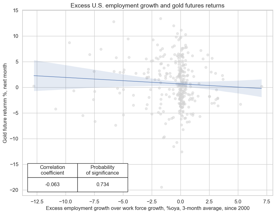
Plausibly, there should ne a negative predictive relation between U.S. employment growth and gold future returns in USD. That is because strong labor market dynamics by themselves bode for increases in real interests, raising opportunity costs of gold holdings. Indeed, excess employment growth has displayed signficant negative predictive power for gold returns in USD, both at a monthly and quarterly frequency since 2000.
cr_gold = msp.CategoryRelations(
        dfx_gld,
        xcats=["XEMPL_NSA_P1M1ML12_3MMA", "COXR_NSA"],
        cids=["GLD"],
        freq="M",
        lag=1,
        xcat_aggs=["last", "sum"],
        start=start_date,
        xcat_trims=[None, None]
    )


cr_gold.reg_scatter(
    labels=False,
    coef_box="lower left",
    xlab="Excess employment growth over work force growth, %oya, 3-month average, since 2000",
    ylab="Gold future returnm %, next month",
    title="Excess U.S. employment growth and gold futures returns",
    size=(9, 7),
    prob_est="map",
)
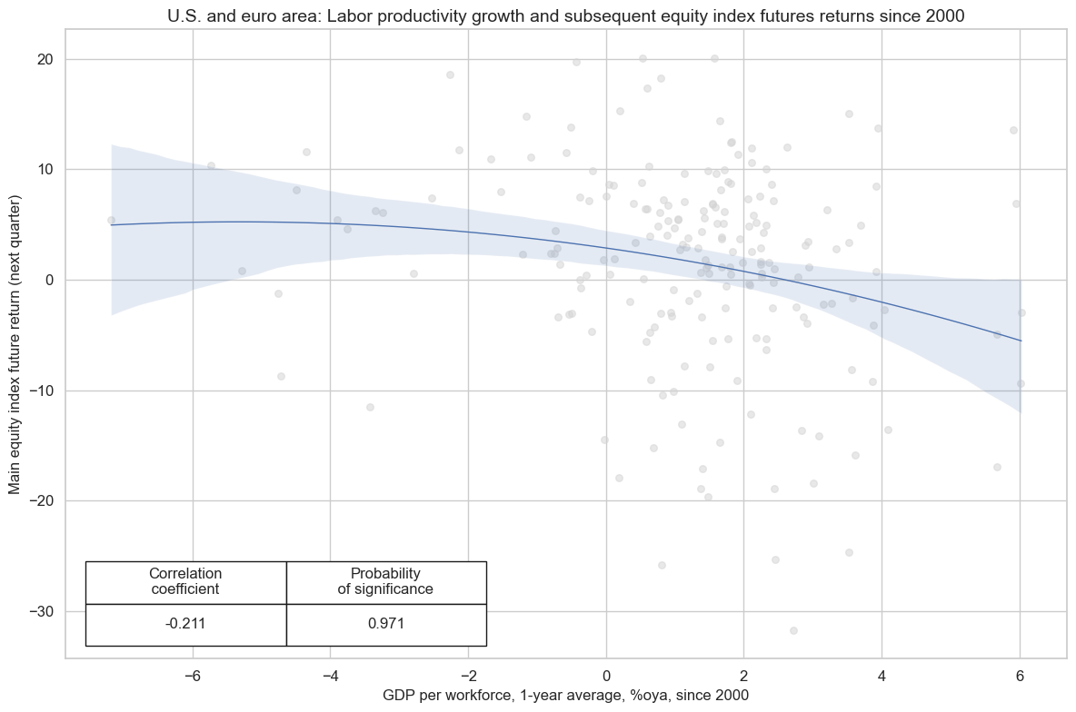
Labor productivity growth has been a clear and significant negative predictor of equity index futures returns in the largest developed markets over the past 25 years. While high productivity growth is positive for profits in and of itself, the conventional calculation of the indicator makes it a bit sluggish, following good news rather than leading it. It also follows economic recoveries and heralds shifts in monetary policy towards tightening and wage pressures.
cr = msp.CategoryRelations(
    dfx,
    xcats=["RGDPPW_SA_P1Q1QL4", "EQXR_NSA"],
    cids=["EUR", "USD"],
    freq="q",
    lag=1,
    xcat_aggs=["last", "sum"],
    fwin=1,
    start="2000-01-01",
    years=None,
    blacklist=None,
)

cr.reg_scatter(
    xlab="GDP per workforce, 1-year average, %oya, since 2000",
    ylab="Main equity index future return (next quarter)",
    title="U.S. and euro area: Labor productivity growth and subsequent equity index futures returns since 2000",
    coef_box="lower left",
    reg_order=2,
    prob_est="map",
    labels=False,
)
Appendices #
Appendix 1: Currency symbols #
The word ‘cross-section’ refers to currencies, currency areas or economic areas. In alphabetical order, these are AUD (Australian dollar), BRL (Brazilian real), CAD (Canadian dollar), CHF (Swiss franc), CLP (Chilean peso), CNY (Chinese yuan renminbi), COP (Colombian peso), CZK (Czech Republic koruna), DEM (German mark), ESP (Spanish peseta), EUR (Euro), FRF (French franc), GBP (British pound), HKD (Hong Kong dollar), HUF (Hungarian forint), IDR (Indonesian rupiah), ITL (Italian lira), JPY (Japanese yen), KRW (Korean won), MXN (Mexican peso), MYR (Malaysian ringgit), NLG (Dutch guilder), NOK (Norwegian krone), NZD (New Zealand dollar), PEN (Peruvian sol), PHP (Phillipine peso), PLN (Polish zloty), RON (Romanian leu), RUB (Russian ruble), SEK (Swedish krona), SGD (Singaporean dollar), THB (Thai baht), TRY (Turkish lira), TWD (Taiwanese dollar), USD (U.S. dollar), ZAR (South African rand).