Demographic trends

This category group contains point-in-time information on latest demographic trends, such as population and work force growth. These often serve as a building block for the calculation of market-relevant macro trends, such as productivity, or as a (partial) benchmark for employment growth and GDP growth.

Population trends

Ticker : POP_NSA_P1Y1YL1 / _P1Q1QL4 / _P1Y1YL1_5YMA / _P1Y1YL1_5YMM / _P1Q1QL4_20QMA / _P1Q1QL4_20QMM

Label : Population growth, %oya: latest year / latest quarter / 5yma / 5ymm / 20qma / 20qmm

Definition : Population growth, % over a year ago: latest year / latest quarter / 5-year moving average / 5-year moving median / 20-quarters moving average / 20-quarters moving median

Notes :

• Population data are taken from national statistics sources. Thus as real time data they include the effects of methodological and territorial changes, such as Russia’s annexation of Crimea.

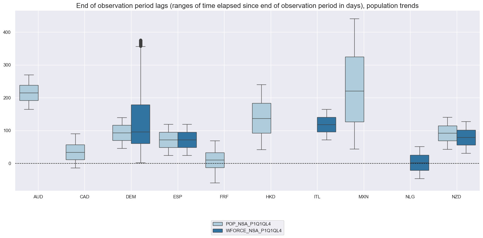
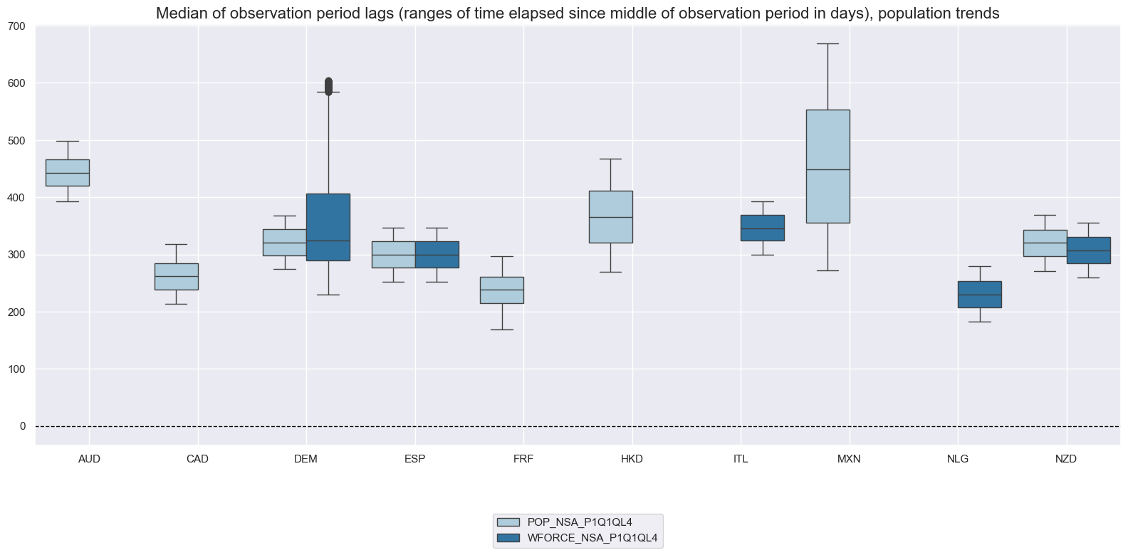
• Most countries release annual-frequency data with publication lags of almost a year. However, a few currency areas release quarterly data: Australia, Canada, Mexico and New Zealand. Hong Kong releases semi-annual data natively but for the purposes of JPMaQS indicators, we have converted it to quarterly data. It is often practical to combine the annual and quarterly series to a common panel, by simple renaming of one of them.

Work force trends

Ticker : WFORCE_NSA_P1Y1YL1 / _P1Q1QL4 / _P1Y1YL1_5YMA / _P1Y1YL1_5YMM / _P1Q1QL4_20QMA / _P1Q1QL4_20QMM

Label : Work force growth, %oya: latest year / latest quarter / 5yma / 5ymm / 20qma / 20qmm

Definition : Work force growth, % over a year ago: latest year / latest quarter / 5-year moving average / 5-year moving median / 20-quarters moving average / 20-quarters moving median

Notes :

• Work force data are taken from national statistics sources and the World Bank.

• Most countries release annual data with almost yearly publication lags. However, the following currency areas release quarterly data: New Zealand. It is often practical to combine the annual and quarterly series to a common panel, by simple renaming of one of them.

Imports

Only the standard Python data science packages and the specialized macrosynergy package are needed.

import os
import numpy as np
import pandas as pd
import matplotlib.pyplot as plt
import seaborn as sns

import macrosynergy.management as msm
import macrosynergy.panel as msp
import macrosynergy.signal as mss
import macrosynergy.pnl as msn
import macrosynergy.visuals as msv

from macrosynergy.download import JPMaQSDownload

import warnings

warnings.simplefilter("ignore")

The JPMaQS indicators we consider are downloaded using the J.P. Morgan Dataquery API interface within the macrosynergy package. This is done by specifying ticker strings , formed by appending an indicator category code <category> to a currency area code <cross_section> . These constitute the main part of a full quantamental indicator ticker, taking the form DB(JPMAQS,<cross_section>_<category>,<info>) , where <info> denotes the time series of information for the given cross-section and category. The following types of information are available:

• value giving the latest available values for the indicator

• eop_lag referring to days elapsed since the end of the observation period

• mop_lag referring to the number of days elapsed since the mean observation period

• grade denoting a grade of the observation, giving a metric of real time information quality.

After instantiating the JPMaQSDownload class within the macrosynergy.download module, one can use the download(tickers,start_date,metrics) method to easily download the necessary data, where tickers is an array of ticker strings, start_date is the first collection date to be considered and metrics is an array comprising the times series information to be downloaded.

cids_dmca = [
    "AUD",
    "CAD",
    "CHF",
    "EUR",
    "GBP",
    "JPY",
    "NOK",
    "NZD",
    "SEK",
    "USD",
]  # DM currency areas
cids_dmec = ["DEM", "ESP", "FRF", "ITL", "NLG"]  # DM euro area countries
cids_latm = ["BRL", "COP", "CLP", "MXN", "PEN"]  # Latam countries
cids_emea = ["CZK", "HUF", "ILS", "PLN", "RON", "RUB", "TRY", "ZAR"]  # EMEA countries
cids_emas = [
    "CNY",
    "HKD",
    "IDR",
    "INR",
    "KRW",
    "MYR",
    "PHP",
    "SGD",
    "THB",
    "TWD",
]  # EM Asia countries
cids_dm = cids_dmca
cids_em = cids_latm + cids_emea + cids_emas
cids = sorted(cids_dm + cids_em)

cids_g3 = ["EUR", "JPY", "USD"]  # DM large currency areas

# For Equity analyses
cids_dmes = ["AUD", "CAD", "CHF", "GBP", "SEK"]  # Smaller DM equity countries
cids_dmeq = cids_g3 + cids_dmes  # DM equity countries

cids_exp = sorted(list(set(cids)))

main = [
    "POP_NSA_P1Y1YL1",
    "POP_NSA_P1Y1YL1_5YMA",
    "POP_NSA_P1Y1YL1_5YMM",
    "POP_NSA_P1Q1QL4_20QMA",
    "POP_NSA_P1Q1QL4_20QMM",
    "POP_NSA_P1Q1QL4",
    "WFORCE_NSA_P1Y1YL1",
    "WFORCE_NSA_P1Q1QL4",
    "WFORCE_NSA_P1Y1YL1_5YMA",
    "WFORCE_NSA_P1Y1YL1_5YMM",
    "WFORCE_NSA_P1Q1QL4_20QMA",
    "WFORCE_NSA_P1Q1QL4_20QMM",
]
econ = [
    "EMPL_NSA_P1M1ML12_3MMA",
    "EMPL_NSA_P1Q1QL4",
    "WAGES_NSA_P1M1ML12_3MMA",
    "WAGES_NSA_P1Q1QL4",
]  # economic context
mark = [
    "EQXR_NSA",
    "FXTARGETED_NSA",
    "FXUNTRADABLE_NSA",
    "DU02YXR_VT10",
    "DU05YXR_VT10",
    "DU02YXR_NSA",
    "DU05YXR_NSA",
]
xcats = main + econ + mark

# Download series from J.P. Morgan DataQuery by tickers

start_date = "1990-01-01"
tickers = [cid + "_" + xcat for cid in cids for xcat in xcats]
print(f"Maximum number of tickers is {len(tickers)}")

# Retrieve credentials

client_id: str = os.getenv("DQ_CLIENT_ID")
client_secret: str = os.getenv("DQ_CLIENT_SECRET")

# Download from DataQuery

with JPMaQSDownload(client_id=client_id, client_secret=client_secret) as downloader:

    df = downloader.download(
        tickers=tickers,
        start_date=start_date,
        metrics=["all"],
        suppress_warning=True,
        show_progress=True,
    )

Maximum number of tickers is 759
Downloading data from JPMaQS.
Timestamp UTC:  2024-04-29 08:57:33
Connection successful!

Requesting data: 100%|██████████| 152/152 [00:32<00:00,  4.68it/s]
Downloading data: 100%|██████████| 152/152 [00:36<00:00,  4.14it/s]

Some expressions are missing from the downloaded data. Check logger output for complete list.
1196 out of 3036 expressions are missing. To download the catalogue of all available expressions and filter the unavailable expressions, set `get_catalogue=True` in the call to `JPMaQSDownload.download()`.
Some dates are missing from the downloaded data. 
2 out of 8958 dates are missing.

Availability

Most population trend indicators are available by the early 1990s. Notable exceptions are Hungary and South Korea. In comparison, the work force indicators are generally available from the mid-1990s onwards. China is the only cross-section for which work force statistics are available by 1990.

For the explanation of currency symbols, which are related to currency areas or countries for which categories are available, please view Appendix 1 .

xcatx = main

dfd = msm.reduce_df(df, xcats=xcatx, cids=cids_exp)
dfs = msm.check_startyears(
    dfd,
)
msm.visual_paneldates(dfs, size=(20, 5))

plot = msm.check_availability(
    df, xcats=main, cids=cids_exp, start_size=(18, 6), start_years=False
)

The vintage grading of employment and work force data is low, as original vintages are not easily accessible and may need to be restored from printed material. These data are not usually watched by markets.

plot = msp.heatmap_grades(
    df,
    xcats=main,
    cids=cids_exp,
    size=(18, 6),
    title=f"Average vintage grades from {start_date} onwards",
)

xcatx = ["POP_NSA_P1Y1YL1", "WFORCE_NSA_P1Y1YL1"]

msp.view_ranges(
    df,
    xcats=xcatx,
    cids=cids_exp,
    val="eop_lag",
    title="End of observation period lags (ranges of time elapsed since end of observation period in days), population trends",
    start=start_date,
    kind="box",
    size=(16, 8),
)
msp.view_ranges(
    df,
    xcats=xcatx,
    cids=cids_exp,
    val="mop_lag",
    title="Median of observation period lags (ranges of time elapsed since middle of observation period in days), population trends",
    start=start_date,
    kind="box",
    size=(16, 8),
)

For the purpose of the below presentation, we have renamed the quarterly-frequency annual growth rates to yearly-frequency annual growth rates in order to have a full panel of similar measures across most countries.

olds = [
    "POP_NSA_P1Q1QL4",
    "POP_NSA_P1Q1QL4_20QMA",
    "WFORCE_NSA_P1Q1QL4",
    "WFORCE_NSA_P1Q1QL4_20QMA",
    "WAGES_NSA_P1Q1QL4",
    "EMPL_NSA_P1Q1QL4",
]
news = [
    "POP_NSA_P1Y1YL1",
    "POP_NSA_P1Y1YL1_5YMA",
    "WFORCE_NSA_P1Y1YL1",
    "WFORCE_NSA_P1Y1YL1_5YMA",
    "WAGES_NSA_P1M1ML12_3MMA",
    "EMPL_NSA_P1M1ML12_3MMA",
]

dfx = df.replace(to_replace=olds, value=news)

scols = ["cid", "xcat", "real_date", "value"]
dfx = dfx[scols].copy().sort_values(["cid", "xcat", "real_date"])
dfx["ticker"] = dfx["cid"] + "_" + dfx["xcat"]

History

Population growth

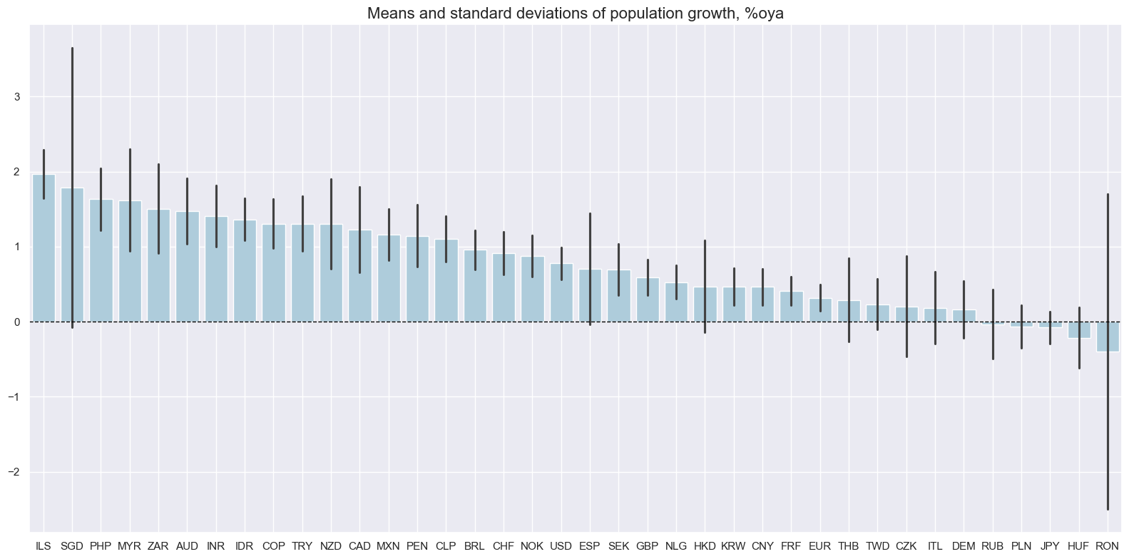
Average population growth has been between 2% and just below -0.5% across the set of relevant markets. Romania, in particular, displays a significant population decline.

xcatx = ["POP_NSA_P1Y1YL1"]

msp.view_ranges(
    df,
    xcats=xcatx,
    cids=cids_exp,
    sort_cids_by="mean",
    title="Means and standard deviations of population growth, %oya",
    start="2000-01-01",
)

xcatx = ["POP_NSA_P1Y1YL1", "POP_NSA_P1Y1YL1_5YMA"]

msp.view_timelines(
    df,
    xcats=xcatx,
    cids=cids_exp,
    start="2000-01-01",
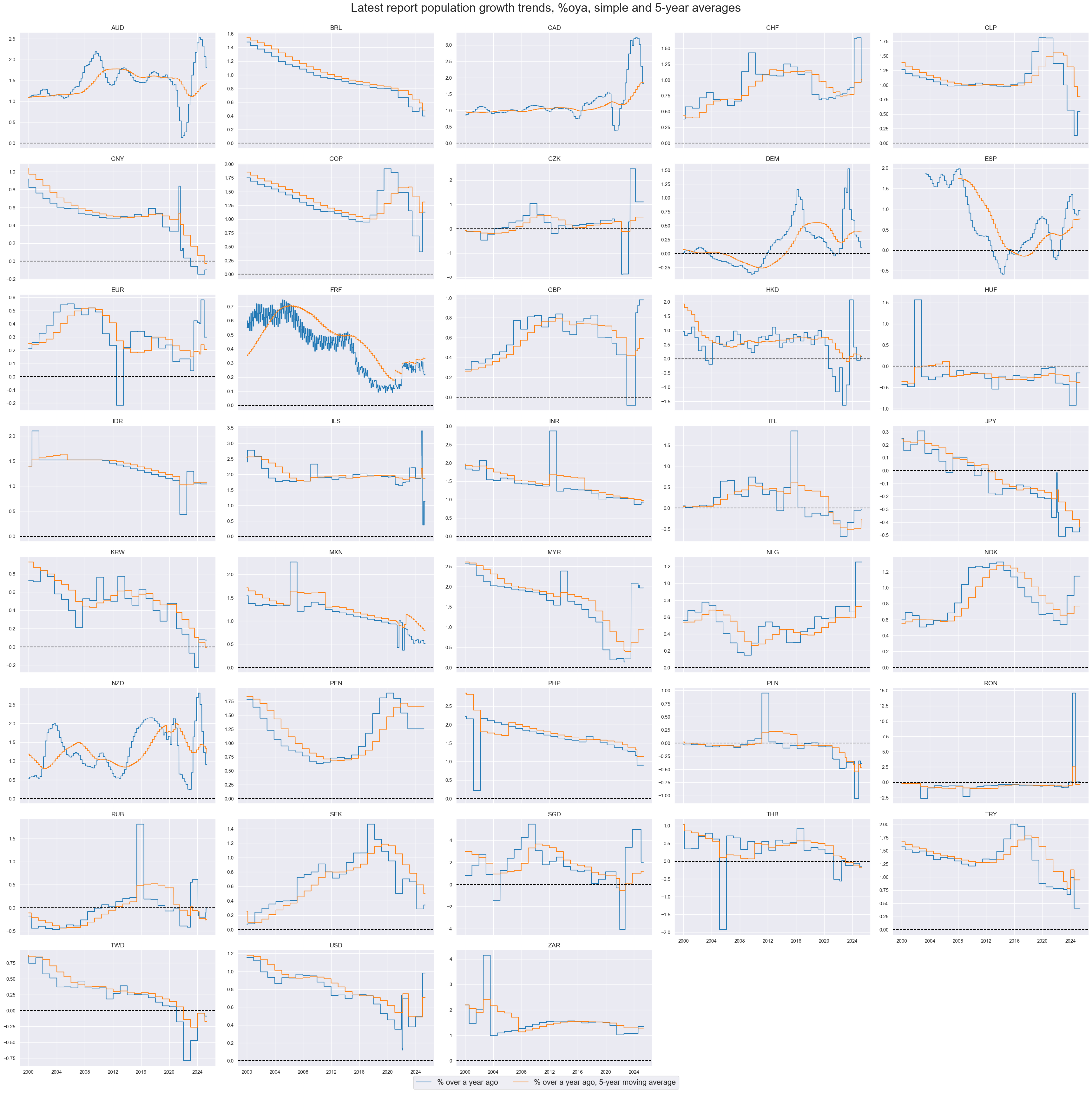
    title="Latest report population growth trends, %oya, simple and 5-year averages",
    xcat_labels=["% over a year ago", "% over a year ago, 5-year moving average"],
    title_fontsize=27,
    legend_fontsize=17,
    ncol=5,
    same_y=False,
    all_xticks=True,
)

Work force growth

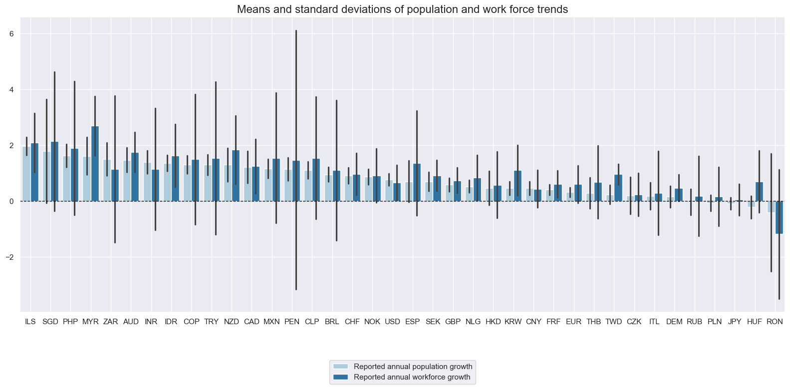
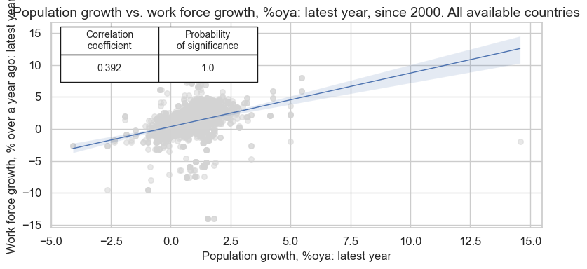
While there is an obvious and clear relation between population and workforce growth in the medium term, there are also notable differences. In relative terms, the country with the higher population growth does not always record a more rapid expansion of the workforce. Romania displays both considerable negative population and workforce growth. Majority of other countries on average achieved positive workforce growth since 2000.

xcatx = ["POP_NSA_P1Y1YL1", "WFORCE_NSA_P1Y1YL1"]

msp.view_ranges(
    dfx,
    xcats=xcatx,
    cids=cids_exp,
    sort_cids_by="mean",
    start="2000-01-01",
    title="Means and standard deviations of population and work force trends",
    xcat_labels=[
        "Reported annual population growth",
        "Reported annual workforce growth",
    ],
)

cr_pop_wf = msp.CategoryRelations(
    dfx,
    xcats=["POP_NSA_P1Y1YL1", "WFORCE_NSA_P1Y1YL1"],
    cids=cids,
    freq="Q",
    lag=0,
    xcat_aggs=["last", "last"],
    start="2000-01-01",
)

cr_pop_wf.reg_scatter(
    labels=False,
    coef_box="upper left",
    xlab="Population growth, %oya: latest year",
    ylab="Work force growth, % over a year ago: latest year",
    title="Population growth vs. work force growth, %oya: latest year, since 2000. All available countries",
    size=(8, 4),
    prob_est="map",
)

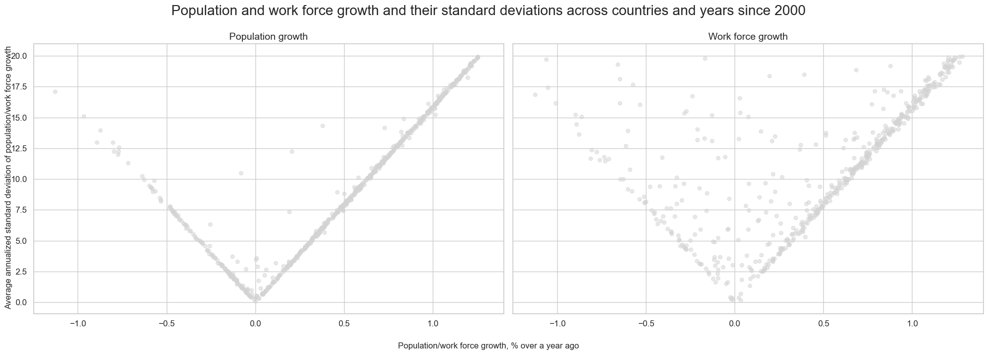
There has been a clear linear relation between average population growth and its standard deviation, across currency areas and years. This suggests high absolute population growth comes with high uncertainty.

dfa = msp.historic_vol(
    dfx, xcat="POP_NSA_P1Y1YL1", cids=cids, lback_meth="xma", postfix="_ASD"
)
dfx = msm.update_df(dfx, dfa)

dfa = msp.historic_vol(
    dfx, xcat="WFORCE_NSA_P1Y1YL1", cids=cids, lback_meth="xma", postfix="_ASD"
)
dfx = msm.update_df(dfx, dfa)


cr_pop_vol = msp.CategoryRelations(
    dfx,
    xcats=["POP_NSA_P1Y1YL1", "POP_NSA_P1Y1YL1_ASD"],
    cids=cids,
    freq="A",
    lag=0,
    xcat_trims=[20, 20],
    xcat_aggs=["mean", "mean"],
    start="2000-01-01",
)

cr_wf_vol = msp.CategoryRelations(
    dfx,
    xcats=["WFORCE_NSA_P1Y1YL1", "WFORCE_NSA_P1Y1YL1_ASD"],
    cids=cids,
    freq="A",
    lag=0,
    xcat_aggs=["mean", "mean"],
    xcat_trims=[20, 20],
    start="2000-01-01",
)

msv.multiple_reg_scatter(
    [cr_pop_vol, cr_wf_vol],
    title="Population and work force growth and their standard deviations across countries and years since 2000",
    xlab="Population/work force growth, % over a year ago",
    ylab="Average annualized standard deviation of population/work force growth",
    figsize=(20, 7),
    prob_est="map",
    fit_reg=False,
    coef_box=None,
    subplot_titles=["Population growth", "Work force growth"],
)

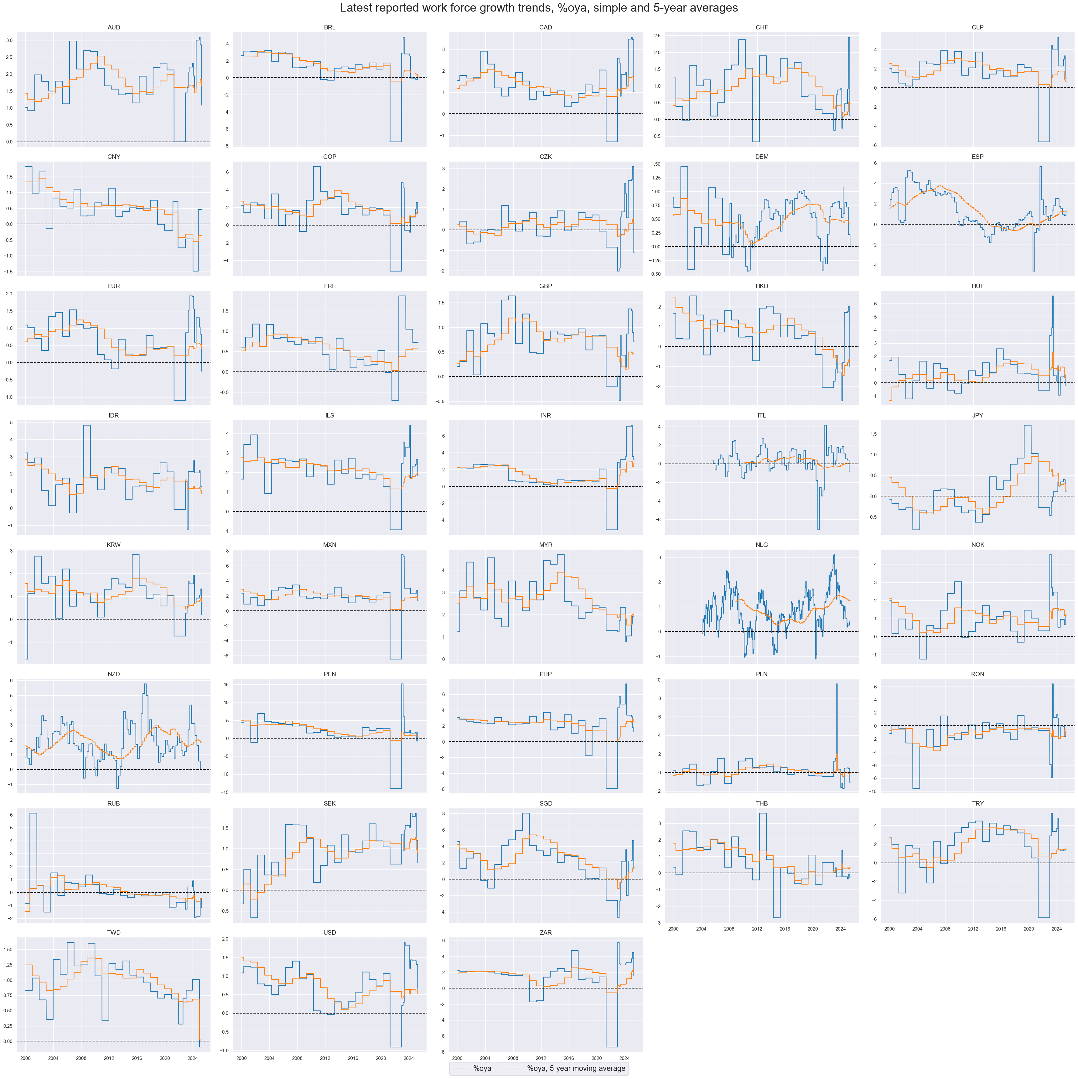
Annual work force growth can be very volatile from year-to-year. Meaningful trends require multi-year averaging.

xcatx = ["WFORCE_NSA_P1Y1YL1", "WFORCE_NSA_P1Y1YL1_5YMA"]

msp.view_timelines(
    dfx,
    xcats=xcatx,
    cids=cids_exp,
    start="2000-01-01",
    title="Latest reported work force growth trends, %oya, simple and 5-year averages",
    xcat_labels=["%oya", "%oya, 5-year moving average"],
    title_fontsize=27,
    legend_fontsize=17,
    ncol=5,
    same_y=False,
    all_xticks=True,
)

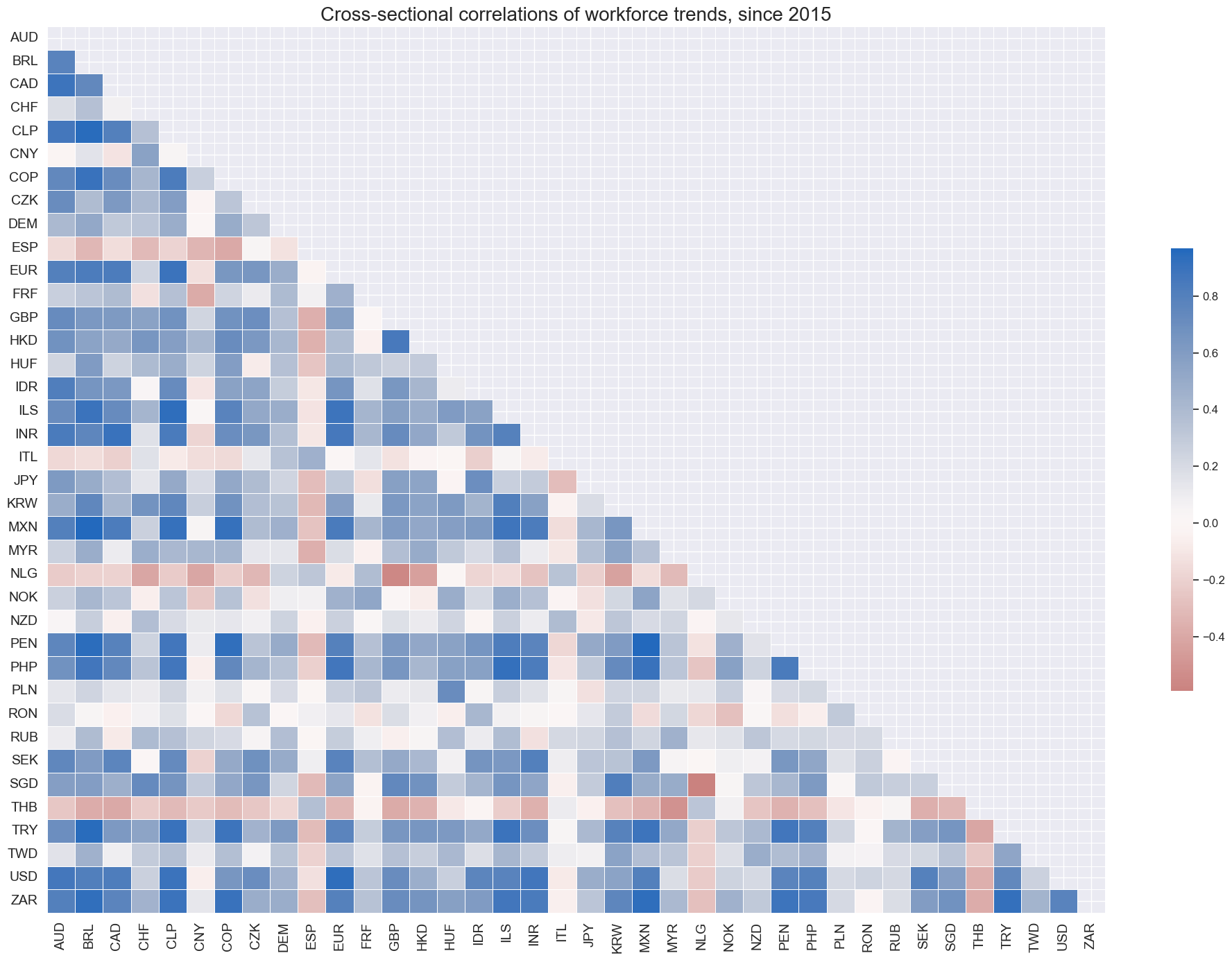
Since 2015, Thailand has stood out as the one country maintaining a negative correlation with global workforce growth.

msp.correl_matrix(
    dfx,
    xcats="WFORCE_NSA_P1Y1YL1",
    # xcats=["WFORCE_NSA_P1Y1YL1", "POP_NSA_P1Y1YL1"],
    cids=cids,
    title="Cross-sectional correlations of workforce trends, since 2015",
    size=(20, 14),
    start="2015-01-01",
)

Importance

Research links

On demographic trends and equity returns:

“Strong household spending, wage growth, and labor markets mark, all other things equal, unfavorable macro conditions for equity performance. Conversely, strengthening corporate profitability, cheap labor, and monetary policy support would mark favorable conditions.” Macrosynergy post

“[There is] strong empirical evidence that demographic changes predict future excess returns in international data, but the U.S. evidence is very weak…The demographic variables that predict U.S. excess returns are not the same ones that predict excess returns on other countries…The most powerful predictive demographic variable for international excess returns is the change in the proportion of retired people, as a fraction of the adult population.” A Ang and A Maddaloni

“Using demographic projections, the traditional predictive regression can be augmented to include predicted values of the contemporaneous valuation predictor. We show that this can improve both pseudo and true out-of-sample stock return prediction at the five-year horizon.” Gospodinov, Maynard, Pesavento

“High employment growth should, on its own, indicate a shift of monetary policy towards higher policy rates, a shift in labour market conditions towards stronger wage trends, and a shift in the inflation outlook towards upside risks. All of these shifts would be unfavourable for equity markets. Hence, if financial markets are not fully information efficient, we would expect that concurrent information on positive excess employment growth forecasts negative broad equity market return trends while information on a shortfall in employment growth predicts positive equity return trends.” Jobs growth as trading signal

On demographic trends and FX returns:

“High employment growth supports tighter monetary policy and greater tolerance for currency strength on the part of the central bank. It is also often indicative of strong competitiveness of an economy. Hence, we should expect that, all other things equal, countries with relatively strong employment growth post positive FX forward returns.” Jobs growth as trading signal

On demographic trends and real estate:

“Changes in the number of births over time lead to large and predictable changes in the demand for housing. These changes in housing demand appear to have substantial impact on the price of housing. “ G Mankiw and D Weil

On demographic trends and fixed income:

“We find that the safe real rate in the United States has statistically and economically important long-run correlations with aggregate labor hours and demographic variables.” K Lunsford and K West

“… demographic variables play an important role in the determination of the low frequency movements in the the real returns of financial assets through individual’s saving decisions, explaining nearly 50 percent of the variance of the annual real returns of Treasury bills.” WP of FEDERAL RESERVE BANK OF ST. LOUIS

The main channel through which demographics affect the real interest rate is the increase in life expectancy. At all stages of their life cycle, individuals save more to finance consumption over a longer time horizon. C. Carvalho et al

“Demographic changes affect nominal yields mainly through real bond yields…The strength of the demographic effect on real yields explains cross-country differences in the comovement between stock and bond markets.” Gozluklu and Morin On demographic trends and economic variables:

“Demographic change can influence the underlying growth rate of the economy, structural productivity growth, living standards, savings rates, consumption, and investment; it can influence the long-run unemployment rate and equilibrium interest rate, housing market trends, and the demand for financial assets.” Federal Reserve Bank of Cleveland

“We find a positive long-run relationship between the euro area core inflation (HICP excluding energy and food) and the growth rate of the working-age population as a share of the total population.” IMF Working paper

“Demographics account for a decrease in the natural real interest rate of about 1.4 percentage points in the euro area compared with the average for the 1980s to 2030 under the baseline calibration. Two channels prevail in providing the downward impact: the increasing scarcity of effective labor input and the growing willingness of individuals to save due to longer life expectancy.” Papetti

Demographic trends indicators are often combined with employment, wage and GDP growth statistics to estimate excess employment, wage and labor productivity growth trends. They are used, for example, in the following Macrosynergy posts:

• Jobs growth as trading signal

• Equity market timing: the value of consumption data

• Equity trend following and macro headwinds

• Macroeconomic cycles and asset class returns

• Regression-based macro trading signals

Empirical clues

Demographic trends and equity returns

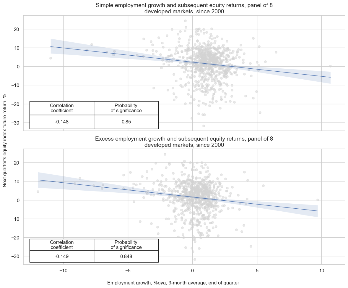
Employment growth has been a negative predictor of subsequent equity index returns in developed markets, consistent with the idea that strong labor markets bode for rising interest rates and wage costs. The probability of significance has been over 90% since 2000 at a quarterly frequency. The relationship becomes more precise and significant, however, if work force growth is considered as well. Looking at “excess employment growth”, i.e., subtracting work force growth from employment growth increase correlation and significance slightly, and provides a meaningful zero threshold, distinguishing between shortfalls and excesses of jobs growth.

calcs = [
    # Excess employment growth
    "EMPLvPOP_NSA_P1M1ML12_3MMA = EMPL_NSA_P1M1ML12_3MMA - POP_NSA_P1Y1YL1_5YMA",  # relative to population growth
    "EMPLvWF_NSA_P1M1ML12_3MMA = EMPL_NSA_P1M1ML12_3MMA - WFORCE_NSA_P1Y1YL1_5YMM",  # relative to workforce growth
]

dfa = msp.panel_calculator(dfx, calcs=calcs, cids=cids_dm, blacklist=None)
dfx = msm.update_df(dfx, dfa)

cr = msp.CategoryRelations(
    dfx,
    xcats=["EMPL_NSA_P1M1ML12_3MMA", "EQXR_NSA"],
    cids=cids_dmeq,
    freq="Q",
    lag=1,
    xcat_aggs=["last", "sum"],
    start="2000-01-01",
)

crx = msp.CategoryRelations(
    dfx,
    xcats=["EMPLvWF_NSA_P1M1ML12_3MMA", "EQXR_NSA"],
    cids=cids_dmeq,
    freq="Q",
    lag=1,
    xcat_aggs=["last", "sum"],
    start="2000-01-01",
)

msv.multiple_reg_scatter(
    [cr, crx],
    subplot_titles=[
        "Simple employment growth and subsequent equity returns, panel of 8 developed markets, since 2000",
        "Excess employment growth and subsequent equity returns, panel of 8 developed markets, since 2000",
    ],
    xlab="Employment growth, %oya, 3-month average, end of quarter",
    ylab="Next quarter's equity index future return, %",
    figsize=(12, 10),
    prob_est="map",
    nrow=2,
    ncol=1,
    coef_box="lower left",
)

Demographic trends as a predictor of IRS returns

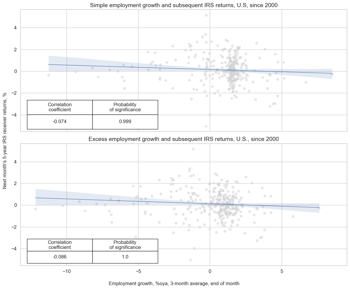
Employment growth has also been a negative predictor of subsequent fixed income returns, albeit there is a dominant influence of the U.S. data and the Federal reserve on global markets. The consideration of work force growth as benchmark for “normal” employment growth has been important for capturing that relation well. Significance of a negative relation between employment growth and subsequent 5-year IRS fixed receiver returns, both at a monthly and quarterly frequency, depends on using excess employment growth rather than simple employment growth.

cr = msp.CategoryRelations(
    dfx,
    xcats=["EMPL_NSA_P1M1ML12_3MMA", "DU05YXR_NSA"],
    cids=["USD"],
    freq="M",
    lag=1,
    xcat_aggs=["last", "sum"],
    start="2000-01-01",
)

crx = msp.CategoryRelations(
    dfx,
    xcats=["EMPLvWF_NSA_P1M1ML12_3MMA", "DU05YXR_NSA"],
    cids=["USD"],
    freq="M",
    lag=1,
    xcat_aggs=["last", "sum"],
    start="2000-01-01",
)

msv.multiple_reg_scatter(
    [cr, crx],
    subplot_titles=[
        "Simple employment growth and subsequent IRS returns, U.S, since 2000",
        "Excess employment growth and subsequent IRS returns, U.S., since 2000",
    ],
    xlab="Employment growth, %oya, 3-month average, end of month",
    ylab="Next month's 5-year IRS receiver returns, %",
    figsize=(12, 10),
    prob_est="map",
    nrow=2,
    ncol=1,
    coef_box="lower left",
)

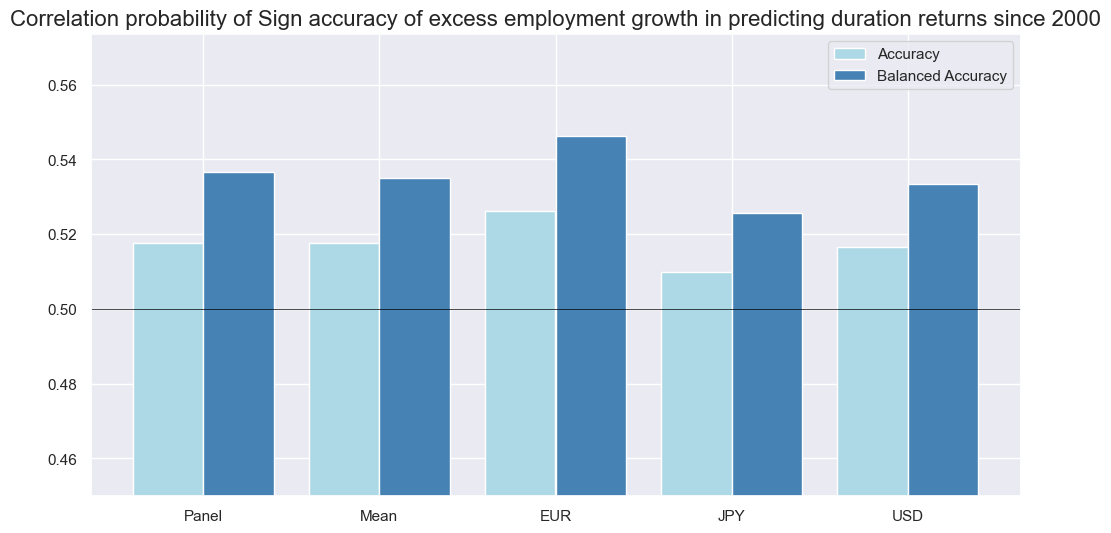
Accuracy and balanced accuracy of the signal from excess employment growth relative to workforce growth exceeds 50% for the three major currencies.

srr = mss.SignalReturnRelations(
    dfx,
    cids=cids_g3,
    sigs="EMPLvWF_NSA_P1M1ML12_3MMA",
    sig_neg=True,
    rets=["DU05YXR_VT10"],
    freqs=["M"],
    start="2000-01-01",
)


srr.accuracy_bars(
    title="Correlation probability of Sign accuracy of excess employment growth in predicting duration returns since 2000",
    size=(12, 6),
)

Appendices

Appendix 1: Currency symbols

The word ‘cross-section’ refers to currencies, currency areas or economic areas. In alphabetical order, these are AUD (Australian dollar), BRL (Brazilian real), CAD (Canadian dollar), CHF (Swiss franc), CLP (Chilean peso), CNY (Chinese yuan renminbi), COP (Colombian peso), CZK (Czech Republic koruna), DEM (German mark), ESP (Spanish peseta), EUR (Euro), FRF (French franc), GBP (British pound), HKD (Hong Kong dollar), HUF (Hungarian forint), INR (Indian rupee), IDR (Indonesian rupiah), ILS (Israeli shekel), ITL (Italian lira), JPY (Japanese yen), KRW (Korean won), MXN (Mexican peso), MYR (Malaysian ringgit), NLG (Dutch guilder), NOK (Norwegian krone), NZD (New Zealand dollar), PEN (Peruvian sol), PHP (Phillipine peso), PLN (Polish zloty), RON (Romanian leu), RUB (Russian ruble), SEK (Swedish krona), SGD (Singaporean dollar), THB (Thai baht), TRY (Turkish lira), TWD (Taiwanese dollar), USD (U.S. dollar), ZAR (South African rand).