PPP exchange rates #
This category group contains information states of purchasing power parity (PPP) exchange rates and related concepts. A PPP exchange rate here is the spot price of a local currency per USD in the spot foreign exchange market that would equalize local and foreign prices. Information states are derived from vintages of (annual) official estimates and subsequent estimations based on relative consumer price index changes.
PPP USD exchange rates #
Ticker : PPPFXRATE_NSA
Label : PPP exchange rate, local currency per USD
Definition : PPP exchange rate, local currency per USD, estimate.
Notes :
-
PPP exchange rates are local currency prices in USD that equate the value of price baskets across currency areas. They are sometimes used as reference for long-term equilibrium exchange rates, following the “law of one price”. Technically, they are ratios of prices in the local currency area to prices in the United States.
-
JPMaQS information states of PPP exchange rates combine annual “official” PPP releases and CPI-based estimates of monthly changes up to the latest month for which CPIs have been released for both the local economy and the United States.
-
There are two official sources of estimation of annual PPP exchange rates: the OECD, for its member states, and the World Bank, for non-OECD countries. The OECD follows the the “Eurostat-OECD” method based on rolling annual special price surveys. The World Bank’s method for non-OECD countries uses irregular price surveys intermittently every few years and estimates other years based on annual GDP deflators. As of October 2023, the last price survey year used for the non-OECD calculations was 2017 and the preceding survey year was 2011. For the exact calculation of annualised PPP conversion factors see Appendix 1 .
-
The methodological differences between OECD and non-OECD explain the more drastic revisions of data vintages for the non-OECD countries. For instance, from 2005, until the next base year, the PPP figures for non-OECD countries were calculated using the extrapolation methodology. Then, in April 2014, the annual observation periods from 2005 were recalculated using the rolling PPP Fisher-type index. In some cases this triggered huge revisions of the originally extrapolated series, because estimation errors that had accumulated over many years were revealed. For further information please see ICP 2011 results were released in April 2014 [worldbank.org] .
-
To estimate at a monthly frequency, we use CPI vintages for the involved currency areas. Then we use a “double price ratio” to estimate and interpolate PPP exchange rates from the latest base year, i.e. the latest year for which official PPP exchange rates have been published. This is the ratio of (1) the local CPI in month m divided by the average CPI of the base year and (2) the local CPI in month m divided by the average CPI of the base year . The calculations are rebased after each new release of annual PPP exchange rates. For details, see the bottom of Appendix 2 .
-
The PPPs under the International Comparison Programme, ICP, have a broad coverage of goods and services, as PPPs are designed to convert the nominal value aggregates in national accounts into real value aggregates. Therefore, the consumption basket used in headline CPI is reasonably well aligned to that of ICP.
-
The Euro series, EUR_PPPFXRATE, will comprise a weighted average of the PPP conversion factors for Italy, France, Germany, Netherlands and Spain. The weights involved in the arithmetic mean will be the nominal GDP. Further, the series will commence from 1999 onwards to reflect the establishment of the Euro. However, for the first three annual observation periods, up until 2003, the PPP calculations for the Euro constituents still used the national currencies in the price relatives. Thus, the PPP figures for the aforementioned years will be multiplied by the fixed nominal exchange to ensure the indicator starts when the currency union was formed.
-
PPP exchange rate series for Romania, Russia and Turkey are adjusted for currency re-denominations in the late 1990s and 2000s.
PPP overvaluation ratio #
Ticker : PPPFXOVERVALUE_NSA
Label : Ratio of market price of currency and PPP-based price (overvaluation ratio)
Definition : Ratio of current market price of currency, based on spot exchange rate, and the estimated PPP-based price.
Notes :
-
A ratio above one indicates local-currency overvaluation versus the USD, based on the PPP exchange rate estimate. A ratio below one indicates undervaluation. A ratio of 1.2, for example, suggests that the local currency is 20% overvalued versus the USD based on the law of one price for comparable baskets.
-
The calculation tracks daily movements in the spot exchange rate relative to the concurrently estimated PPP exchange rate.
PPP excess overvaluation ratios #
Ticker : PPPFXOVERVALUE_NSA_P1MvLTXL1 / _P1DvLTXL1
Label : Excess ratio of market price of currency and PPP: % latest month / % latest day versus expanding long-term median.
Definition : Excess ratio of market price of currency and PPP-based price: % latest month over expanding long-term median since vintage inception lagged by one month / % latest day over expanding long-term median since vintage inception lagged by one day.
Notes :
-
See notes on “PPP overvaluation ratio”.
-
Long-term trends are also calculated based on the latest available full vintage of estimated overvaluation ratios. Latest month means latest 21 days.
-
To differentiate long-term trends from conventional trends, the percentage change will be calculated over an expanding median, as opposed to a moving average of varying time horizons. The expanding median will be lagged by one period (day or month).
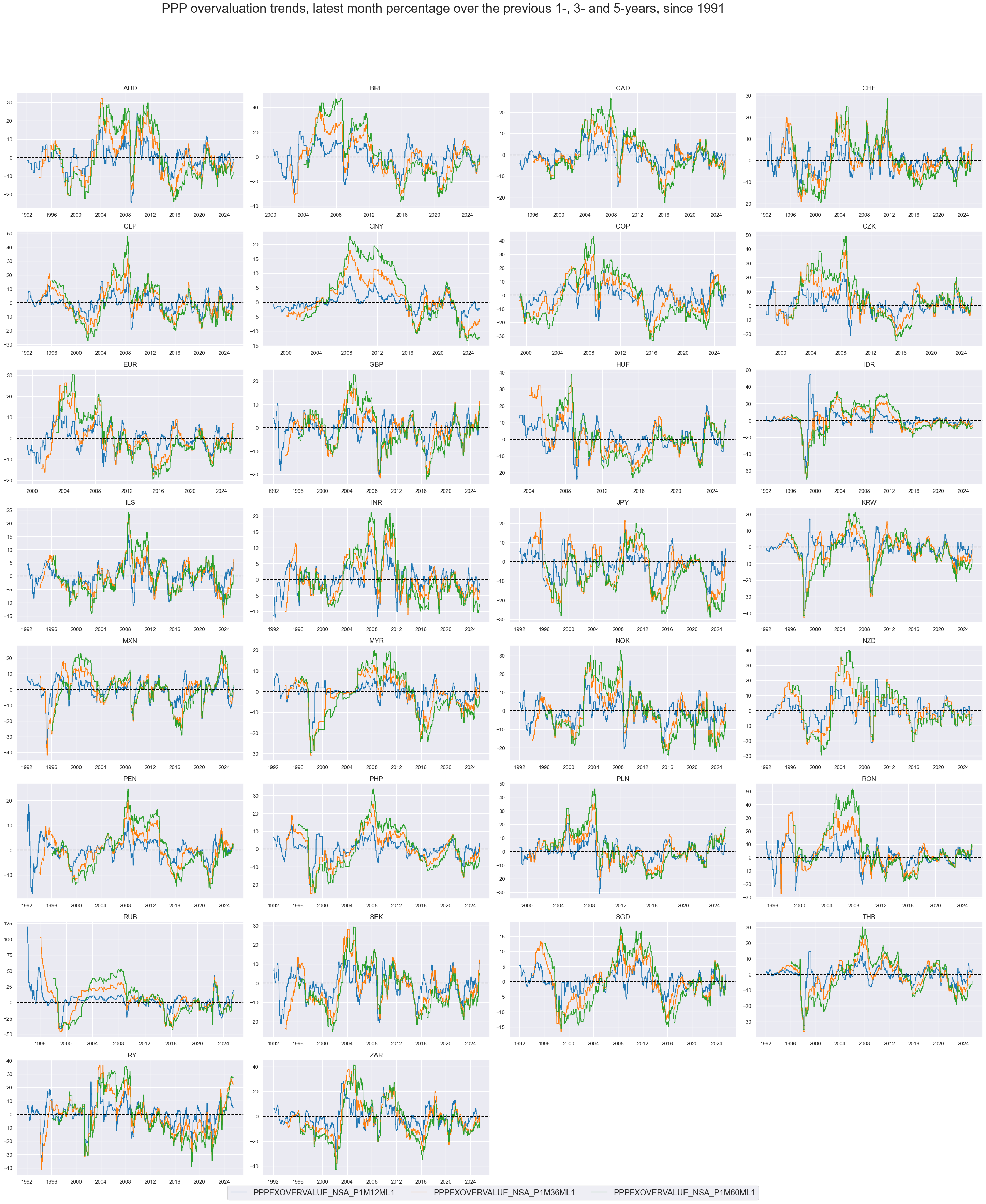
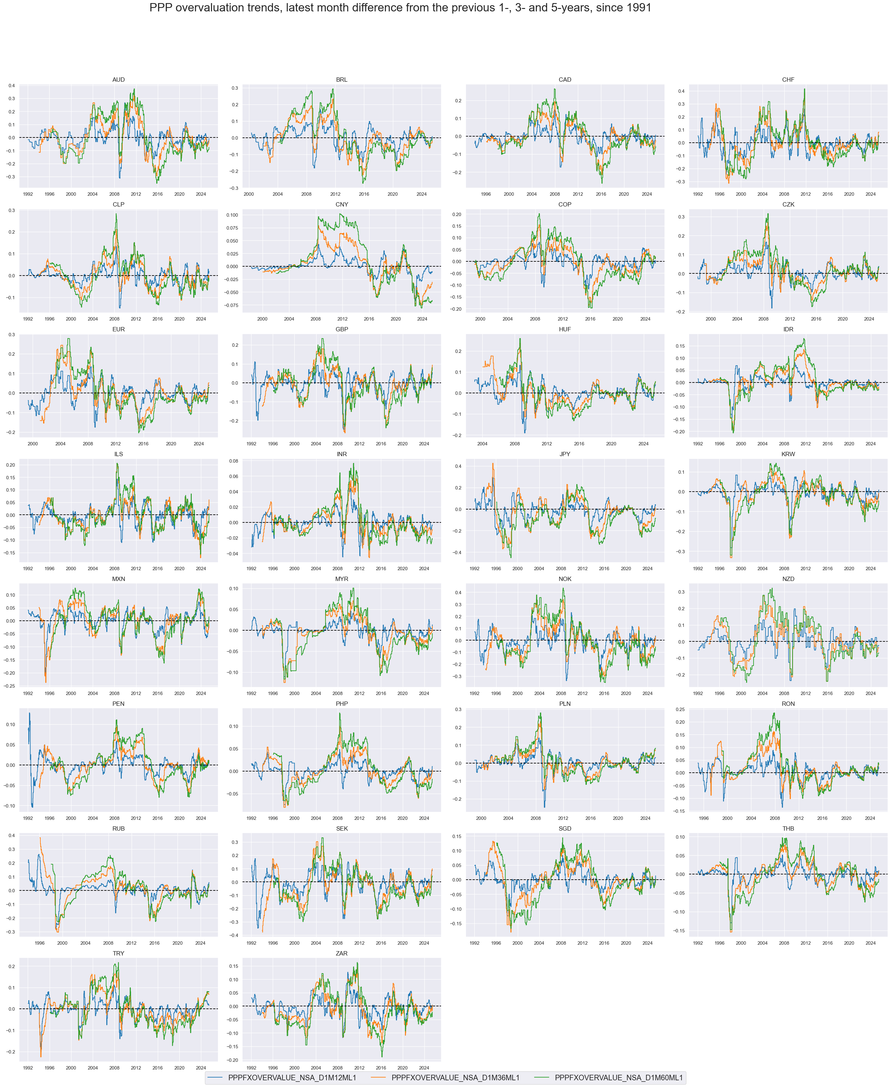
PPP overvaluation ratio trends (monthly frequency) #
Ticker : PPPFXOVERVALUE_NSA_P1M12ML1 / _P1M36ML1 / _P1M60ML1 / _D1M12ML1 / _D1M36ML1 / _D1M60ML1
Label : PPP overvaluation ratio trend: % latest month over previous year / % latest month over the previous 3 years / % latest month over the previous 5 years / difference latest month versus previous year / difference latest month versus previous 3 years / difference latest month versus previous 5 years.
Definition : Trend of ratio of PPP exchange rate to current market FX spot rate based on concurrent vintage: % latest month over previous year / % latest month over the previous 3 years / % latest month over the previous 5 years / difference latest month versus previous year / difference latest month versus previous 3 years / difference latest month versus previous 5 years.
Notes :
-
See notes on “PPP overvaluation ratio”.
-
Trends are all calculated based on the latest available full vintage of estimated overvaluation ratios. Latest month means latest 21 days.
-
Unlike overvaluation ratios, trends tend to fluctuate around their neutral zero level. What they measure is a tendency towards more or less overvaluation or undervaluation. The concept is similar to real trade-weighted appreciation, except that it is based on a more detailed comparison of prices and here the comparison is with the USD alone.
PPP overvaluation ratio trends (daily frequency) #
Ticker : PPPFXOVERVALUE_NSA_P1D260DL1 / _P1D780DL1 / _P1D1300DL1 / _D1D260DL1 / _D1D780DL1 / _D1D1300DL1
Label : PPP overvaluation ratio trend (daily frequency): % latest day over previous year / % latest day over the previous 3 years / % latest day over the previous 5 years / difference latest day versus previous year / difference latest day versus previous 3 years / difference latest day versus previous 5 years.
Definition : Trend of ratio of PPP exchange rate to current market FX spot rate based on concurrent daily vintages: % latest day over previous year / % latest day over the previous 3 years / % latest day over the previous 5 years / difference latest day versus previous year / difference latest day versus previous 3 years / difference latest day versus previous 5 years.
Notes :
-
See notes on “PPP overvaluation ratio”.
-
Trends are all calculated based on the full daily vintages of estimated overvaluation ratios. To create the daily information states, the monthly PPP conversion factor vintages are forward filled between CPI releases or revisions.
Imports #
Only the standard Python data science packages and the specialized
macrosynergy
package are needed.
import os
import numpy as np
import pandas as pd
import matplotlib.pyplot as plt
import seaborn as sns
import math

import json
import yaml

import macrosynergy.management as msm
import macrosynergy.panel as msp
import macrosynergy.signal as mss
import macrosynergy.pnl as msn


from macrosynergy.download import JPMaQSDownload

from timeit import default_timer as timer
from datetime import timedelta, date, datetime

import warnings

warnings.simplefilter("ignore")
The
JPMaQS
indicators we consider are downloaded using the J.P. Morgan Dataquery API interface within the
macrosynergy
package. This is done by specifying
ticker strings
, formed by appending an indicator category code
<category>
to a currency area code
<cross_section>
. These constitute the main part of a full quantamental indicator ticker, taking the form
DB(JPMAQS,<cross_section>_<category>,<info>)
, where
<info>
denotes the time series of information for the given cross-section and category. The following types of information are available:
-
valuegiving the latest available values for the indicator -
eop_lagreferring to days elapsed since the end of the observation period -
mop_lagreferring to the number of days elapsed since the mean observation period -
gradedenoting a grade of the observation, giving a metric of real time information quality.
After instantiating the
JPMaQSDownload
class within the
macrosynergy.download
module, one can use the
download(tickers,start_date,metrics)
method to easily download the necessary data, where
tickers
is an array of ticker strings,
start_date
is the first collection date to be considered and
metrics
is an array comprising the times series information to be downloaded.
# Cross-sections of interest

cids_dm = [
    "AUD",
    "CAD",
    "CHF",
    "EUR",
    "GBP",
    "JPY",
    "NOK",
    "NZD",
    "SEK",
    "USD",
]  # DM currency areas

cids_latm = ["BRL", "COP", "CLP", "MXN", "PEN"]  # Latam countries
cids_emea = ["CZK", "HUF", "ILS", "PLN", "RON", "RUB", "TRY", "ZAR"]  # EMEA countries
cids_emas = [
    "CNY",
    "IDR",
    "INR",
    "KRW",
    "MYR",
    "PHP",
    "SGD",
    "THB",
]  # EM Asia countries

cids_em = cids_latm + cids_emea + cids_emas

cids = sorted(cids_dm + cids_em)
cids_ppp = sorted(list(set(cids) - set(["USD"])))
main = [
    "PPPFXRATE_NSA",
    "PPPFXOVERVALUE_NSA",
    "PPPFXOVERVALUE_NSA_P1M12ML1",
    "PPPFXOVERVALUE_NSA_P1M36ML1",
    "PPPFXOVERVALUE_NSA_P1M60ML1",
    "PPPFXOVERVALUE_NSA_D1M12ML1",
    "PPPFXOVERVALUE_NSA_D1M36ML1",
    "PPPFXOVERVALUE_NSA_D1M60ML1",
    "PPPFXOVERVALUE_NSA_P1MvLTXL1",
    "PPPFXOVERVALUE_NSA_P1D260DL1",
    "PPPFXOVERVALUE_NSA_P1D780DL1",
    "PPPFXOVERVALUE_NSA_P1D1300DL1",
    "PPPFXOVERVALUE_NSA_D1D260DL1",
    "PPPFXOVERVALUE_NSA_D1D780DL1",
    "PPPFXOVERVALUE_NSA_D1D1300DL1",
    "PPPFXOVERVALUE_NSA_P1DvLTXL1",
]
econ = [
    "REER_NSA_P1W4WL1",
    "REER_NSA_P1M12ML1",
    "REER_NSA_P1M60ML1",
    "RIR_NSA",
]  # economic context
mark = [
    "FXXR_NSA",
    "FXXRUSD_NSA",
    "FXXR_VT10",
    "FXXRHvGDRB_NSA",
    "FXCRR_NSA",
    "FXCRR_VT10",
    "DU02YXR_NSA",
    "DU05YXR_NSA",
]  # market links

xcats = main + econ + mark
# Download series from J.P. Morgan DataQuery by tickers

start_date = "1990-01-01"
tickers = [cid + "_" + xcat for cid in cids for xcat in xcats]
print(f"Maximum number of tickers is {len(tickers)}")

# Retrieve credentials

client_id: str = os.getenv("DQ_CLIENT_ID")
client_secret: str = os.getenv("DQ_CLIENT_SECRET")

# Download from DataQuery

with JPMaQSDownload(client_id=client_id, client_secret=client_secret) as downloader:
    start = timer()
    df = downloader.download(
        tickers=tickers,
        start_date=start_date,
        show_progress=True,
        metrics=["value", "eop_lag", "mop_lag", "grading"],
        suppress_warning=True,
    )
    end = timer()

dfd = df

print("Download time from DQ: " + str(timedelta(seconds=end - start)))
Maximum number of tickers is 868
Downloading data from JPMaQS.
Timestamp UTC:  2025-06-25 10:33:37
Connection successful!
Requesting data: 100%|██████████| 174/174 [00:39<00:00,  4.38it/s]
Downloading data: 100%|██████████| 174/174 [01:31<00:00,  1.89it/s]
Some expressions are missing from the downloaded data. Check logger output for complete list.
112 out of 3472 expressions are missing. To download the catalogue of all available expressions and filter the unavailable expressions, set `get_catalogue=True` in the call to `JPMaQSDownload.download()`.
Download time from DQ: 0:02:24.747293
Availability #
cids_exp = cids_ppp  # cids expected in category panels
msm.missing_in_df(dfd, xcats=main, cids=cids_exp)
No missing XCATs across DataFrame.
Missing cids for PPPFXOVERVALUE_NSA:             []
Missing cids for PPPFXOVERVALUE_NSA_D1D1300DL1:  []
Missing cids for PPPFXOVERVALUE_NSA_D1D260DL1:   []
Missing cids for PPPFXOVERVALUE_NSA_D1D780DL1:   []
Missing cids for PPPFXOVERVALUE_NSA_D1M12ML1:    []
Missing cids for PPPFXOVERVALUE_NSA_D1M36ML1:    []
Missing cids for PPPFXOVERVALUE_NSA_D1M60ML1:    []
Missing cids for PPPFXOVERVALUE_NSA_P1D1300DL1:  []
Missing cids for PPPFXOVERVALUE_NSA_P1D260DL1:   []
Missing cids for PPPFXOVERVALUE_NSA_P1D780DL1:   []
Missing cids for PPPFXOVERVALUE_NSA_P1DvLTXL1:   []
Missing cids for PPPFXOVERVALUE_NSA_P1M12ML1:    []
Missing cids for PPPFXOVERVALUE_NSA_P1M36ML1:    []
Missing cids for PPPFXOVERVALUE_NSA_P1M60ML1:    []
Missing cids for PPPFXOVERVALUE_NSA_P1MvLTXL1:   []
Missing cids for PPPFXRATE_NSA:                  []
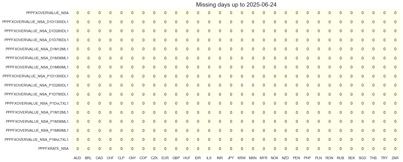
Real-time monthly quantamental indicators of PPP exchange rate are available from 1991 for most of the countries. The main exceptions are Brazil, Columbia, China, Czech Republic and the Eurozone which are all available from 1999.
For the explanation of currency symbols, which are related to currency areas or countries for which categories are available, please view Appendix 3 .
xcatx = main

cidx = cids_exp

dfx = msm.reduce_df(dfd, xcats=xcatx, cids=cidx)
dfs = msm.check_startyears(
    dfx,
)
msm.visual_paneldates(dfs, size=(18, 6))

print("Last updated:", date.today())

Last updated: 2025-06-25
xcatx = main
cidx = cids_exp

plot = msm.check_availability(
    dfd, xcats=xcatx, cids=cids_exp, start_size=(18, 6), start_years=False
)
The PPP exchange rate indicators have high grading since all data are based on source vintages.
xcatx = main
cidx = cids_exp

plot = msp.heatmap_grades(
    dfd,
    xcats=xcatx,
    cids=cidx,
    size=(18, 6),
    title=f"Average vintage grades from {start_date} onwards",
)

xcatx = ["PPPFXRATE_NSA"]
cidx = cids_exp

msp.view_ranges(
    dfd,
    xcats=xcatx,
    cids=cidx,
    val="eop_lag",
    title="End of observation period lags (ranges of time elapsed since end of observation period in days)",
    start="1995-01-01",
    kind="box",
    size=(16, 4),
)

msp.view_ranges(
    dfd,
    xcats=xcatx,
    cids=cidx,
    val="mop_lag",
    title="End of observation period lags (ranges of time elapsed since end of observation period in days)",
    start="1995-01-01",
    kind="box",
    size=(16, 4),
)


History #
PPP exchange rate series #
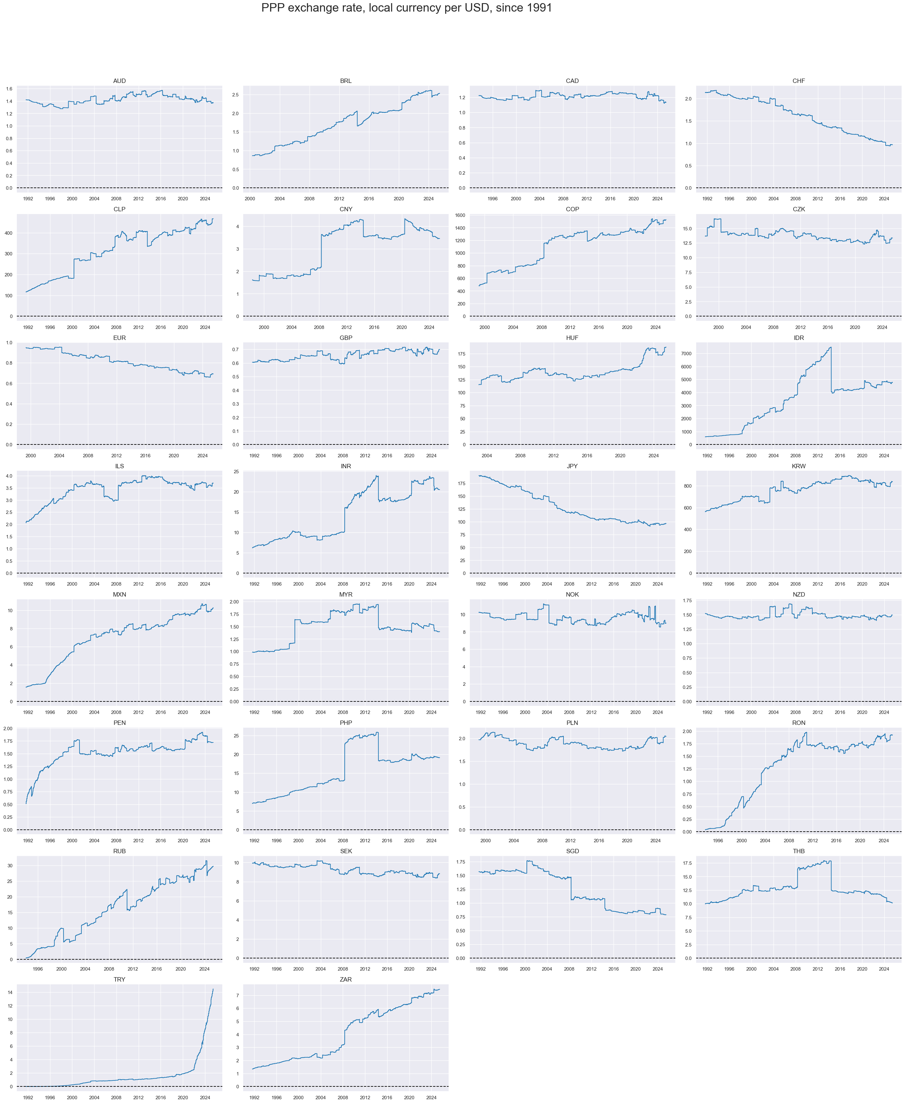
PPP exchange rates of developed or emerging countries countries with similar inflation rates to the U.S. have been fairly stationary. Emerging countries with higher inflation rates have naturally seen an upward drift in the USD price in local currency. Low inflation or deflation countries, such as Switzerland and Japan have experienced a downward drift.
The data also show the effect of the World Bank’s revision cycle, with a number of sharp upward and downward shifts in EM PPP exchange rates on the days of publication.
xcatx = ["PPPFXRATE_NSA"]
cidx = cids_exp

msp.view_timelines(
    dfd,
    xcats=xcatx,
    cids=cidx,
    start="1991-01-01",
    title="PPP exchange rate, local currency per USD, since 1991",
    title_adj=1.03,
    title_xadj=0.45,
    label_adj=0.075,
    title_fontsize=27,
    legend_fontsize=17,
    ncol=4,
    same_y=False,
    size=(12, 7),
    aspect=1.7,
    all_xticks=True,
)
PPP overvaluation ratio #
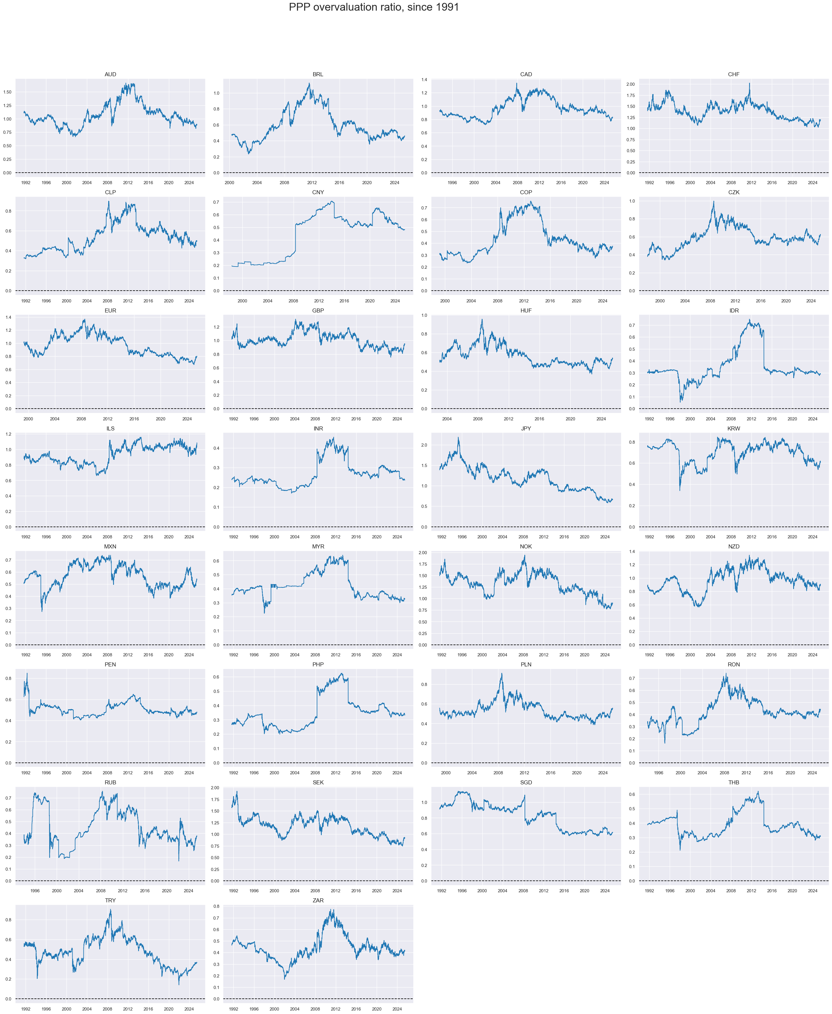
Overvaluation ratios have been stationary in the long-term. This suggests that PPP exchange rates have exerted some long-term “gravity” on spot exchange rates: price differences may have remained but they did not drift apart on a sustained basis. Exceptions were Japan and Singapore, but even in these countries the residual drift was gentle.
xcatx = ["PPPFXOVERVALUE_NSA"]
cidx = cids_exp

msp.view_timelines(
    dfd,
    xcats=xcatx,
    cids=cidx,
    start="1991-01-01",
    title="PPP overvaluation ratio, since 1991",
    title_adj=1.03,
    title_xadj=0.45,
    label_adj=0.075,
    title_fontsize=27,
    legend_fontsize=17,
    ncol=4,
    same_y=False,
    size=(12, 7),
    aspect=1.7,
    all_xticks=True,
)
PPP excess overvaluation ratios #
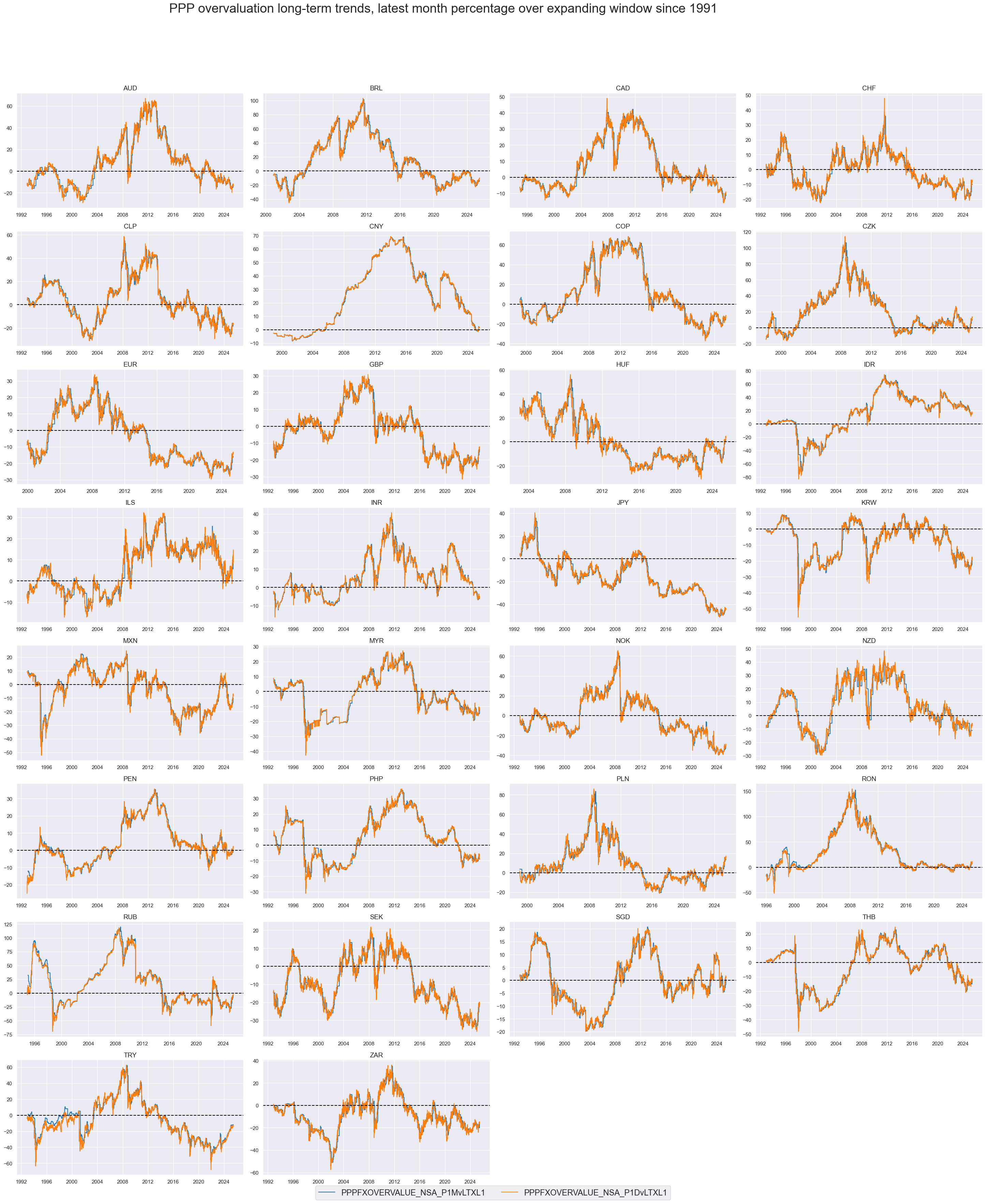
Excess overvaluation ratios track the part of ratios of currency prices to PPP-based prices that is above the long-term average since vintage inception. Excessed ratios are naturally closer to zero than simple overvaluation ratios and typically stationary.
xcatx = ["PPPFXOVERVALUE_NSA_P1MvLTXL1", "PPPFXOVERVALUE_NSA_P1DvLTXL1"]

cidx = cids_exp

msp.view_timelines(
    dfd,
    xcats=xcatx,
    cids=cidx,
    start="1991-01-01",
    title="PPP overvaluation long-term trends, latest month percentage over expanding window since 1991",
    title_adj=1.03,
    title_xadj=0.45,
    label_adj=0.075,
    title_fontsize=27,
    legend_fontsize=17,
    ncol=4,
    same_y=False,
    size=(12, 7),
    aspect=1.7,
    all_xticks=True,
)
PPP overvaluation trends #
Overvaluation trends naturally are more stationary metrics of valuation, implicitly assuming that lookback averages of valuation ratios form a neutral lever or a level that the economy has grown accustomed to.
xcatx = [
    "PPPFXOVERVALUE_NSA_P1M12ML1",
    "PPPFXOVERVALUE_NSA_P1M36ML1",
    "PPPFXOVERVALUE_NSA_P1M60ML1",
]
cidx = cids_exp

msp.view_timelines(
    dfd,
    xcats=xcatx,
    cids=cidx,
    start="1991-01-01",
    title="PPP overvaluation trends, latest month percentage over the previous 1-, 3- and 5-years, since 1991",
    title_adj=1.03,
    title_xadj=0.45,
    label_adj=0.075,
    title_fontsize=27,
    legend_fontsize=17,
    ncol=4,
    same_y=False,
    size=(12, 7),
    aspect=1.7,
    all_xticks=True,
)
xcatx = [
    "PPPFXOVERVALUE_NSA_D1M12ML1",
    "PPPFXOVERVALUE_NSA_D1M36ML1",
    "PPPFXOVERVALUE_NSA_D1M60ML1",
]
cidx = cids_exp

msp.view_timelines(
    dfd,
    xcats=xcatx,
    cids=cidx,
    start="1991-01-01",
    title="PPP overvaluation trends, latest month difference from the previous 1-, 3- and 5-years, since 1991",
    title_adj=1.03,
    title_xadj=0.45,
    label_adj=0.075,
    title_fontsize=27,
    legend_fontsize=17,
    ncol=4,
    same_y=False,
    size=(12, 7),
    aspect=1.7,
    all_xticks=True,
)
Importance #
Research links #
“Our reading of the literature leads us to the main conclusions that purchasing power parity might be viewed as a valid long-run international parity condition when applied to bilateral exchange rates obtaining among major industrialised countries, and that mean reversion in real exchange rates displays significant nonlinearities” Lucio Sarno and Mark P. Taylor
“Over the past ten years, research on purchasing power parity has enjoyed a rebirth… The main positive result is that there does seem to be long-run convergence to PPP, though further work on the issue of survivorship bias would be valuable. Also, the most convincing evidence on long-run convergence to PPP still comes from data sets that employ at least some fixed-rate data.” Kenneth Froot and Kenneth Rogoff
“The proposition that nominal and real exchange rates are volatile when allowed to float freely, and hence deviate from their long-run level, has become something of a stylized fact in international finance. There is now growing evidence, however, to suggest that although purchasing power parity does not hold in the short-term, it does hold as a long-run phenomenon. The main explanation is that if the predominant force upsetting the PPP relationship is nominal, or monetary, it will only have a transitory effect on deviations from PPP.” Tamim Bayoumi and Ronald MacDonald
Empirical clues #
Exclude periods of exchange rates pegs or untradable forward/NDF market.
dfb = dfd[dfd["xcat"].isin(["FXTARGETED_NSA", "FXUNTRADABLE_NSA"])].loc[
    :, ["cid", "xcat", "real_date", "value"]
]
dfba = (
    dfb.groupby(["cid", "real_date"])
    .aggregate(value=pd.NamedAgg(column="value", aggfunc="max"))
    .reset_index()
)
dfba["xcat"] = "FXBLACK"
fxblack = msp.make_blacklist(dfba, "FXBLACK")
Overvaluation ratios #
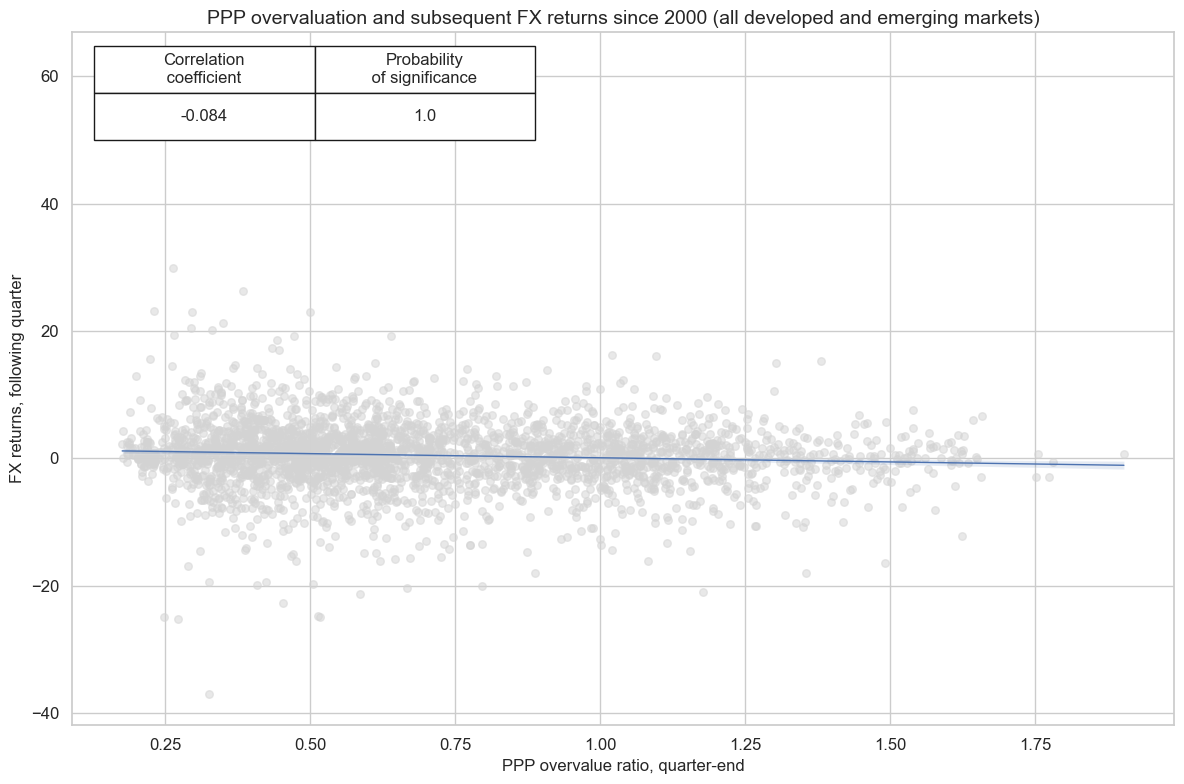
In line with general intuition, there has been signficant negative correlation between overaluation ratios and subsequent FX forward returns at a monthly, quarterly or annual horizon. This holds true for both the developed and emerging markets.
xcatx = ["PPPFXOVERVALUE_NSA", "FXXR_NSA"]
cidx = cids_ppp

cr = msp.CategoryRelations(
    dfd,
    xcats=xcatx,
    cids=cidx,
    freq="Q",
    lag=1,
    xcat_aggs=["last", "sum"],
    start="2000-01-01",
    blacklist=fxblack,
)

cr.reg_scatter(
    title="PPP overvaluation and subsequent FX returns since 2000 (all developed and emerging markets)",
    labels=False,
    coef_box="upper left",
    ylab="FX returns, following quarter",
    xlab="PPP overvalue ratio, quarter-end",
    prob_est="map",
)
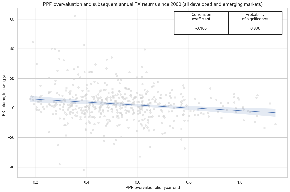
In accordance with its reputation as a long-term indicator, the overvaluation ratio’s predictive power shows particularly well at longer horizons, such as 1 year ahead.
xcatx = ["PPPFXOVERVALUE_NSA", "FXXR_NSA"]
cidx = cids_em

cr = msp.CategoryRelations(
    dfd,
    xcats=xcatx,
    cids=cidx,
    freq="A",
    lag=1,
    xcat_aggs=["last", "sum"],
    start="2000-01-01",
    blacklist=fxblack,
)

cr.reg_scatter(
    title="PPP overvaluation and subsequent annual FX returns since 2000 (all developed and emerging markets)",
    labels=False,
    coef_box="upper right",
    ylab="FX returns, following year",
    xlab="PPP overvalue ratio, year-end",
    prob_est="map",
)
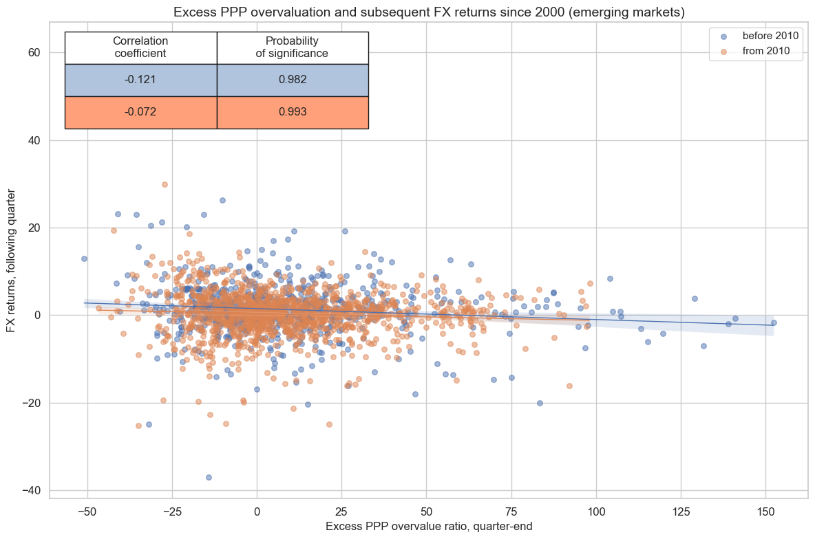
Excess overvaluation ratios, as opposed to simple overvaluation ratios, are particularly important as predictors of emerging markets FX returns. Unlike simple overvaluation ratios they do not imply structural long or short positions across currencies. There has been a significant negative predictive relation between excess overvaluation and subsequent EM FX returns in the 2000s as well as in the 2010s and 2020s.
xcatx = ["PPPFXOVERVALUE_NSA_P1MvLTXL1", "FXXR_NSA"]
cidx = cids_em

cr = msp.CategoryRelations(
    dfd,
    xcats=xcatx,
    cids=cidx,
    freq="Q",
    lag=1,
    xcat_aggs=["last", "sum"],
    start="2000-01-01",
    blacklist=fxblack,
)

cr.reg_scatter(
    title="Excess PPP overvaluation and subsequent FX returns since 2000 (emerging markets)",
    labels=False,
    coef_box="upper left",
    ylab="FX returns, following quarter",
    xlab="Excess PPP overvalue ratio, quarter-end",
    separator=2010,
    prob_est="map",
)
Overvaluation ratio trends #
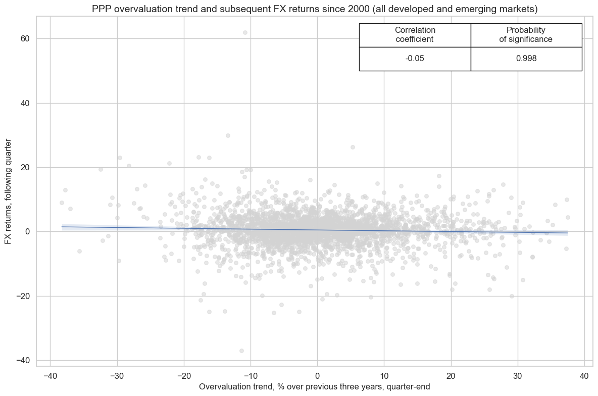
Overvaluation trends have displayed less predictive forward correlation than overvaluation ratios. However, the predictive relation has still been negative and significant and may thus be a valid counterweight to a standard trend-following signal.
xcatx = ["PPPFXOVERVALUE_NSA_P1M36ML1", "FXXR_NSA"]
cidx = cids_ppp

cr = msp.CategoryRelations(
    dfd,
    xcats=xcatx,
    cids=cidx,
    freq="Q",
    lag=1,
    xcat_aggs=["last", "sum"],
    start="2000-01-01",
    blacklist=fxblack,
)

cr.reg_scatter(
    title="PPP overvaluation trend and subsequent FX returns since 2000 (all developed and emerging markets)",
    labels=False,
    coef_box="upper right",
    ylab="FX returns, following quarter",
    xlab="Overvaluation trend, % over previous three years, quarter-end",
    prob_est="map",
)
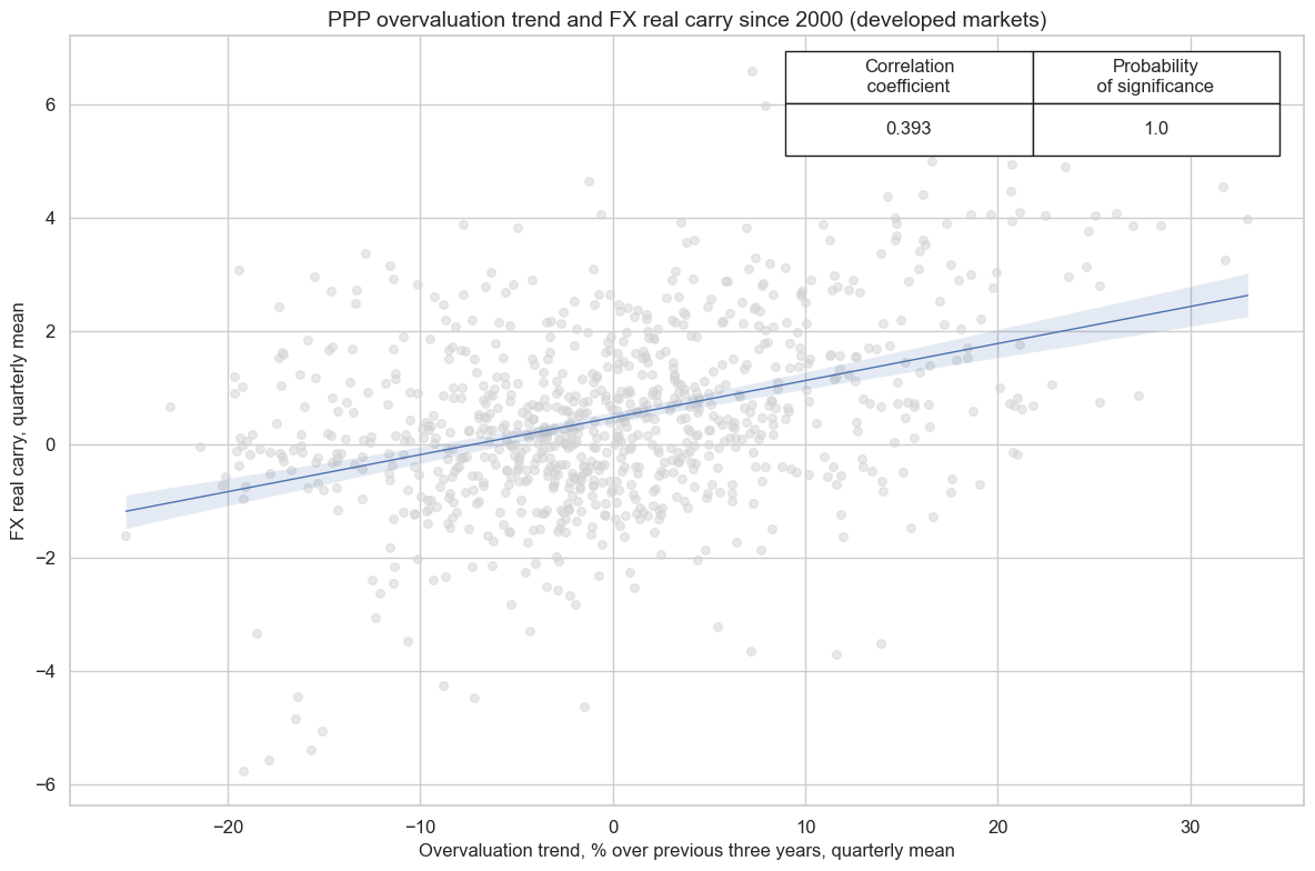
In the developed world there has been a strong concurrent positive relation between real FX forward carry and overvaluation trends. This suggests that in a normal mode, relatively high real interest rates, i.e., tight monetary policy, coincides with a stronger currency.
xcatx = ["PPPFXOVERVALUE_NSA_P1M36ML1", "FXCRR_NSA"]
cidx = cids_dm

cr = msp.CategoryRelations(
    dfd,
    xcats=xcatx,
    cids=cidx,
    freq="Q",
    lag=0,
    xcat_aggs=["mean", "mean"],
    start="2000-01-01",
    blacklist=fxblack,
)

cr.reg_scatter(
    title="PPP overvaluation trend and FX real carry since 2000 (developed markets)",
    labels=False,
    coef_box="upper right",
    ylab="FX real carry, quarterly mean",
    xlab="Overvaluation trend, % over previous three years, quarterly mean",
    prob_est="map",
)
PPPFXOVERVALUE_NSA_P1M36ML1 misses: ['USD'].
FXCRR_NSA misses: ['USD'].
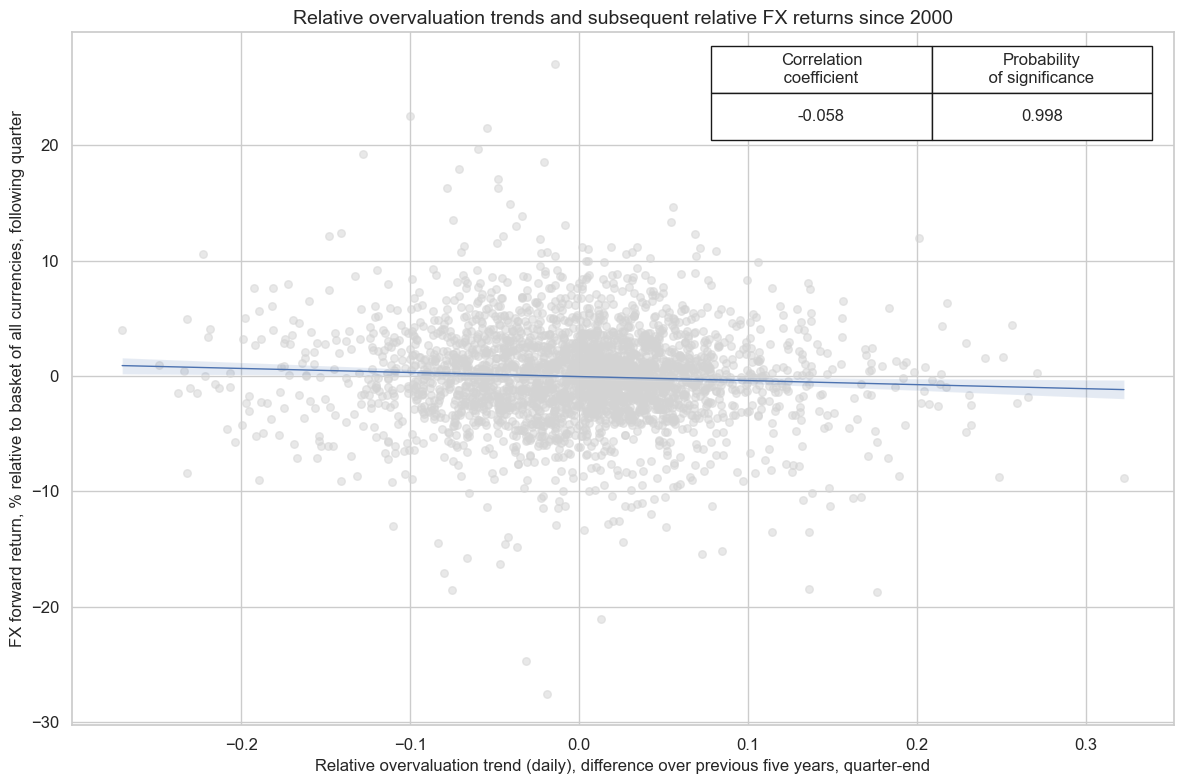
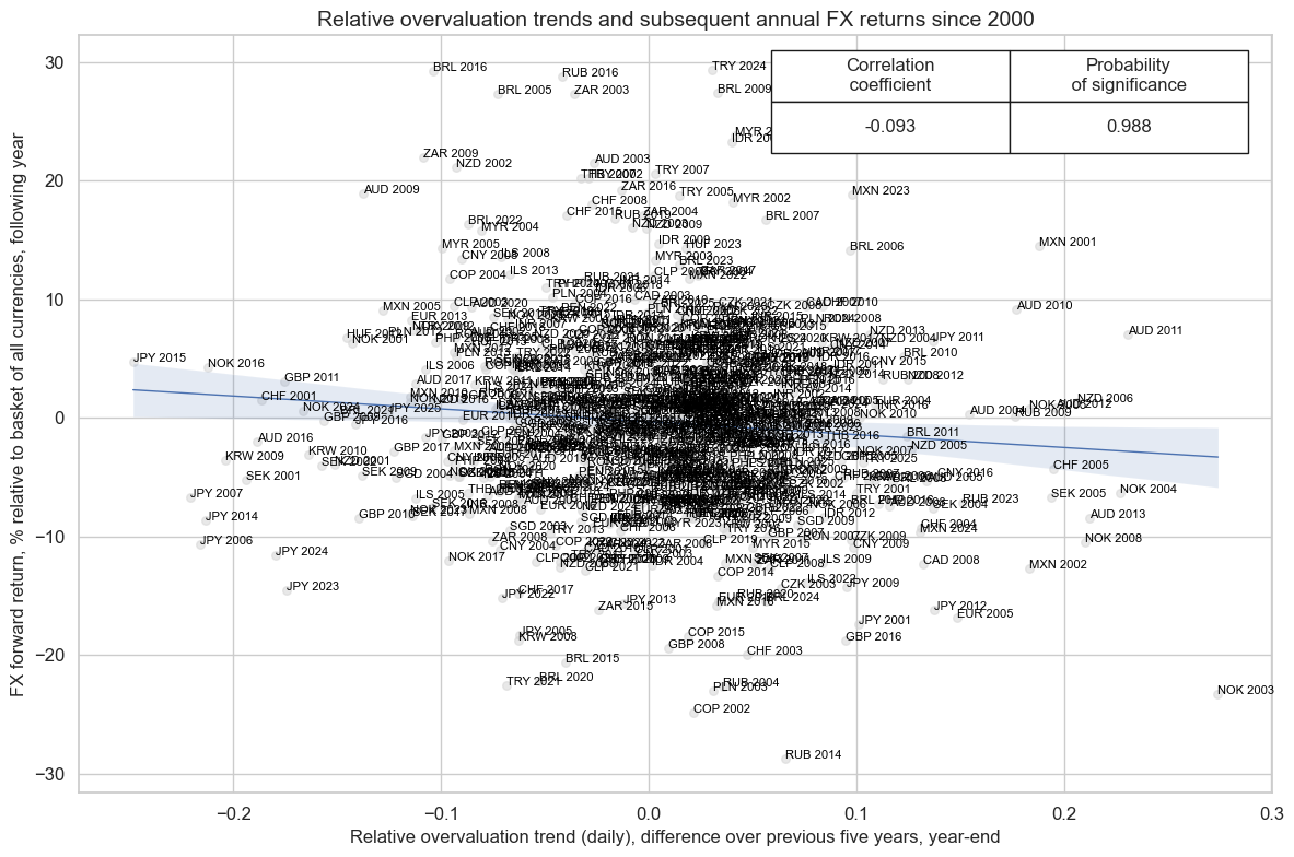
Importantly, the negative predictive power of overvaluation trends for FX returns also applies on a relative basis.This analysis compares one currency versus all others, as opposed to just the USD. Relative overvaluation trends have been significant negative predictors of subsequent relative FX forward returns at various frequencies and lookback periods.
xc = "PPPFXOVERVALUE_NSA_D1D1300DL1"  # "PPPFXOVERVALUE_NSA_P1D1300DL1" # "PPPFXOVERVALUE_NSA_D1M60ML1"
xcatx = [xc, "FXXR_NSA"]
cidx = cids_ppp

dfa = msp.make_relative_value(dfd, xcats=xcatx, cids=cidx, postfix="_RV")

dfxx_agg = msm.update_df(dfd, dfa)

cr = msp.CategoryRelations(
    dfxx_agg,
    xcats=[f"{xc}_RV", "FXXR_NSA_RV"],
    cids=cidx,
    freq="Q",
    lag=1,
    xcat_aggs=["last", "sum"],
    start="2000-01-01",
    blacklist=fxblack,
    xcat_trims=[2, 30],  # trim for better graphic focus
)

cr.reg_scatter(
    title="Relative overvaluation trends and subsequent relative FX returns since 2000",
    labels=False,
    coef_box="upper right",
    ylab="FX forward return, % relative to basket of all currencies, following quarter",
    xlab="Relative overvaluation trend (daily), difference over previous five years, quarter-end",
    prob_est="map",
)
xc = "PPPFXOVERVALUE_NSA_D1M60ML1"
xcatx = [xc, "FXXR_NSA"]
cidx = cids_ppp

dfa = msp.make_relative_value(dfd, xcats=xcatx, cids=cidx, postfix="_RV")

dfxx_agg = msm.update_df(dfd, dfa)

cr = msp.CategoryRelations(
    dfxx_agg,
    xcats=[f"{xc}_RV", "FXXR_NSA_RV"],
    cids=cidx,
    freq="A",
    lag=1,
    xcat_aggs=["last", "sum"],
    start="2000-01-01",
    blacklist=fxblack,
    xcat_trims=[2, 30],  # trim for better graphic focus
)

cr.reg_scatter(
    title="Relative overvaluation trends and subsequent annual FX returns since 2000",
    labels=True,
    coef_box="upper right",
    ylab="FX forward return, % relative to basket of all currencies, following year",
    xlab="Relative overvaluation trend (daily), difference over previous five years, year-end",
    prob_est="map",
)
Appendix 1: How official annual purchasing power parity exchange rates are calculated #
Conceptually, PPP exchange rates are ratios of prices for comparable goods and services in local and foreign currency areas. They are exchange rates for which comparable goods and services would cost the same in both places.
PPP exchange rates are based on a Fisher-type index whereby the aggregate PPP exchange rate level is a weighted average of elementary PPP exchange rate levels. Each elementary PPP exchange rate represents a basic heading, covering similar goods and services across areas. An example of a basic heading would be wine which is disaggregated into the three groups: red wine, white wine and sparkling wine. At the elementary level, basket indices do not use weights and a geometric mean is calculated. The prices used for the elementary PPP exchange rates are annual averages. Index number formulae beyond the elementary level are derived using systems of weights. Thus, to produce the aggreate PPP exchange rate, the procedure is broken into three steps: i) a matrix of Laspeyres-type PPP exchange rates; ii) a matrix of Paasche-type PPP exchange rates; iii) a geometric mean of the two, a matrix of Fisher-type PPP exchange rates.
For detailed methodological notes, please see here .
Appendix 2: How JPMaQS monthly purchasing power parity indices are calculated #
Higher-frequency PPP indices are estimated based on price index ratios, which is principally a standard procedure in the literature:
-
https://en.wikipedia.org/wiki/Purchasing_power_parity
-
https://ec.europa.eu/eurostat/web/products-manuals-and-guidelines/-/ks-ra-12-023
Here the estimate of monthly PPP exchange rates based on annual releases uses point-in-time estimates of CPI ratios. The last release of PPP will be multiplied by a ratio of CPIs between the local currency area and the U.S. with the average of the CPI ratio set to 1 for the last available official annual PPP survey. Thus, the calculation takes three steps:
First, for monthly estimation we use CPI “double ratios”: Those are the ratios of (1) local currency CPI at a given month to the average CPI for the last reported PPP year relative to (2) U.S. CPI for the same month to the average CPI for the last reported PPP year. Average here means the arithmetic mean of CPI over the 12 months of the last reported PPP year (T).
This choice of CPI base reflects that PPP exchange rates of the OECD and World Bank are based on annual averages of the surveyed prices.
The double CPI ratio applied for PPP exchange rate estimation for month m is first calculated as the ratio of change in the CPI index for the local currency to the 12-month base year mean. As a measure of change in the PPP exchange rate, we take the ratio of this local currency change in index to the USD change in the CPI index relative to the base year. Lastly, we multiply this double ratio with the latest official annual PPP exchange rate to obtain the month PPP exchange rate estimate.
The above calculation will be completed for each new monthly release up until the next annual release for PPP exchange rate at \((T + 1)\) . This applies to both forward estimation and (backward) interpolation for monthly PPP exchange rates.
Following \((T + 1)\) ’s release, the described sequence of calculations will be applied to the new base year to give a new vintage; the monthly PPP exchange rates will use \((T + 1)\) as the base year.
Appendix 3: Currency symbols #
The word ‘cross-section’ refers to currencies, currency areas or economic areas. In alphabetical order, these are AUD (Australian dollar), BRL (Brazilian real), CAD (Canadian dollar), CHF (Swiss franc), CLP (Chilean peso), CNY (Chinese yuan renminbi), COP (Colombian peso), CZK (Czech Republic koruna), DEM (German mark), ESP (Spanish peseta), EUR (Euro), FRF (French franc), GBP (British pound), HKD (Hong Kong dollar), HUF (Hungarian forint), IDR (Indonesian rupiah), ITL (Italian lira), JPY (Japanese yen), KRW (Korean won), MXN (Mexican peso), MYR (Malaysian ringgit), NLG (Dutch guilder), NOK (Norwegian krone), NZD (New Zealand dollar), PEN (Peruvian sol), PHP (Phillipine peso), PLN (Polish zloty), RON (Romanian leu), RUB (Russian ruble), SEK (Swedish krona), SGD (Singaporean dollar), THB (Thai baht), TRY (Turkish lira), TWD (Taiwanese dollar), USD (U.S. dollar), ZAR (South African rand).