Private credit expansion #
This category group includes metrics of the expansion of private credit (local convention) with statistical adjustment for jumps and spikes in the series’, based on concurrently available vintages. Adjustments for outliers are particularly important for these series’, due to the occasional distortionary influences of legal and regulatory changes.
Nominal private credit growth #
Ticker : PCREDITBN_SJA_P1M1ML12
Label : Private bank credit, seasonally- and jump-adjusted, % oya.
Definition : Private bank credit at the end of the latest reported month, seasonally and jump-adjusted, % change over a year ago
Notes :
-
For most countries, the indicator is limited to bank loans to private households and companies.
-
The stock of credit is denominated in local currency.
-
Jump adjustment means that two types of outliers are adjusted for. Firstly, large “spikes” (i.e. two subsequent large moves of the seasonal index in opposite directions) are averaged. Holiday patterns or tax effects can be responsible for these spikes. Secondly, large one-off jumps in the index are replaced by the local trend. The causes of one-off jumps can be balance sheet restructurings in the banking systems and tax-related asset shifts. The criteria for adjustments are statistical, based on pattern recognition. For more information, see Appendix 1 .
Changes in nominal private credit growth #
Ticker : PCREDITBN_SJA_P1M1ML12_D1M1ML12 / _P1M1ML12_D3M3ML3 / _P1M1ML12_D6M6ML6
Label : Private bank credit, seasonally- and jump-adjusted % oya: diff m/m / diff 3m/3m / diff 6m/6m.
Definition : Private bank credit at the end of the latest reported month, seasonally and jump-adjusted, % change over a year ago: difference of last month over previous month / difference of last 3 months over previous 3 months / difference of last 6 months over previous 6 months
Notes :
-
These indicators record quantamental changes in private credit growth, not changes in information states.
-
See the important notes under “Nominal private credit growth”.
Private credit expansion as % of GDP #
Ticker : PCREDITGDP_SJA_D1M1ML12
Label : Banks’ private credit expansion, seasonally- and jump-adjusted, as % of GDP over 1 year.
Definition : Change of private credit over 1 year ago, seasonally and jump-adjusted, as % of nominal GDP (1-year moving average) in the base period.
Notes :
-
For most countries, the indicator is limited to bank loans to private households and companies.
-
The expansion is calculated as the change in the stock of bank credit over the latest reported 12 months as a % of the annual nominal GDP at the beginning of this 12 month period.
-
Jump adjustment means that two types of outliers are adjusted for. Firstly, large “spikes” (i.e. two subsequent large moves of the seasonal index in opposite directions) are averaged. Holiday patterns or tax effects can be responsible for these spikes. Secondly, large one-off jumps in the index are replaced by the local trend. The causes of one-off jumps can be balance sheet restructurings in the banking systems and tax-related asset shifts. The criteria for adjustments are statistical, based on pattern recognition. For more information, see Appendix 1 .
Changes in private credit expansion #
Ticker : PCREDITGDP_SJA_D1M1ML12_D1M1ML12 / _D1M1ML12_D3M3ML3 / _D1M1ML12_D6M6ML6
Label : Banks’ private credit expansion, seasonally- and jump-adjusted: as % of GDP over 1 year: diff m/m / diff 3m/3m / diff 6m/6m.
Definition : Change of private credit over 1 year ago, seasonally and jump-adjusted: as % of nominal GDP (1-year moving average) in the base period: difference of last month over previous month / difference of last 3 months over previous 3 months / difference of last 6 months over previous 6 months
Notes :
-
These indicators record quantamental changes in private credit expansion, not changes in information states.
-
See the important notes under “Private credit expansion as % of GDP”.
Imports #
Only the standard Python data science packages and the specialized
macrosynergy
package are needed.
import os
import pandas as pd

import macrosynergy.management as msm
import macrosynergy.panel as msp
import macrosynergy.signal as mss
import macrosynergy.pnl as msn
import macrosynergy.visuals as msv

from macrosynergy.download import JPMaQSDownload

from timeit import default_timer as timer
from datetime import timedelta, date

import warnings
from IPython.display import HTML

warnings.simplefilter("ignore")
The
JPMaQS
indicators we consider are downloaded using the J.P. Morgan Dataquery API interface within the
macrosynergy
package. This is done by specifying
ticker strings
, formed by appending an indicator category code
<category>
to a currency area code
<cross_section>
. These constitute the main part of a full quantamental indicator ticker, taking the form
DB(JPMAQS,<cross_section>_<category>,<info>)
, where
<info>
denotes the time series of information for the given cross-section and category.
The following types of information are available:
-
valuegiving the latest available values for the indicator -
eop_lagreferring to days elapsed since the end of the observation period -
mop_lagreferring to the number of days elapsed since the mean observation period -
gradedenoting a grade of the observation, giving a metric of real time information quality.
After instantiating the
JPMaQSDownload
class within the
macrosynergy.download
module, one can use the
            download(tickers,


            start_date,


            metrics)
method to obtain the data. Here
tickers
is an array of ticker strings,
start_date
is the first release date to be considered and
metrics
denotes the types of information requested.
# Cross-sections of interest

cids_dmca = [
    "AUD",
    "CAD",
    "CHF",
    "EUR",
    "GBP",
    "JPY",
    "NOK",
    "NZD",
    "SEK",
    "USD",
]  # DM currency areas
cids_dmec = ["DEM", "ESP", "FRF", "ITL", "NLG"]  # DM euro area countries
cids_latm = ["BRL", "COP", "CLP", "MXN", "PEN"]  # Latam countries
cids_emea = ["CZK", "HUF", "ILS", "PLN", "RON", "RUB", "TRY", "ZAR"]  # EMEA countries
cids_emas = [
    "CNY",
    "HKD",
    "IDR",
    "INR",
    "KRW",
    "MYR",
    "PHP",
    "SGD",
    "THB",
    "TWD",
]  # EM Asia countries

cids_dm = cids_dmca + cids_dmec
cids_em = cids_latm + cids_emea + cids_emas

cids_emeq = ["BRL", 'HKD', "ILS", "INR", "KRW", "MXN", "MYR", "SGD", "THB", "TRY", "TWD", "ZAR"]
cids_dmeq = ['AUD', 'CAD', 'CHF', 'EUR', 'GBP', 'JPY', 'NOK', 'NZD', 'SEK', 'USD']
cids_eq = cids_dmeq + cids_emeq


cids_eueq = ["DEM", "ESP", "FRF", "ITL", "NLG"]
sector_cids = sorted(cids_dmeq + cids_eueq)

cids = sorted(cids_dm + cids_em)
# Quantamental categories of interest

main = [
    "PCREDITBN_SJA_P1M1ML12",
    "PCREDITGDP_SJA_D1M1ML12",
    "PCREDITBN_SJA_P1M1ML12_D1M1ML12",
    "PCREDITBN_SJA_P1M1ML12_D3M3ML3",
    "PCREDITBN_SJA_P1M1ML12_D6M6ML6",
    "PCREDITGDP_SJA_D1M1ML12_D1M1ML12",
    "PCREDITGDP_SJA_D1M1ML12_D3M3ML3",
    "PCREDITGDP_SJA_D1M1ML12_D6M6ML6",
]
econ = ["RIR_NSA", "RGDP_SA_P1Q1QL4_20QMA", "INFTEFF_NSA"]  # economic context

confs = ["CCSCORE_SA_3MMA_D1M1ML12"]
mark = [
    "EQXR_VT10",
    "FXXR_NSA",
    "FXXR_VT10",
    "DU05YXR_VT10",
    "FXTARGETED_NSA",
    "FXUNTRADABLE_NSA",
]  # market links


sector_labels = {
    "ALL": "All sectors",
    "COD": "Cons. discretionary",
    "COS": "Cons. staples",
    "CSR": "Communication services",
    "ENR": "Energy",
    "FIN": "Financials",
    "HLC": "Healthcare",
    "IND": "Industrials",
    "ITE": "Information tech",
    "MAT": "Materials",
    "REL": "Real estate",
    "UTL": "Utilities",
}
sectors = list(sector_labels.keys())
cids_secs = list(sector_labels.keys())[1:]

vt_xrets = ["EQC" + sec + "XR_VT10" for sec in sectors]
untradable = ['EQC' + sec + 'UNTRADABLE_NSA' for sec in sectors]

eqret = vt_xrets + untradable #+ simple_xrets


xcats = main + econ + mark+ confs+ eqret
# Download series from J.P. Morgan DataQuery by tickers

start_date = "1990-01-01"
tickers = [cid + "_" + xcat for cid in cids for xcat in xcats]
print(f"Maximum number of tickers is {len(tickers)}")

# Retrieve credentials

client_id: str = os.getenv("DQ_CLIENT_ID")
client_secret: str = os.getenv("DQ_CLIENT_SECRET")

# Download from DataQuery

with JPMaQSDownload(client_id=client_id, client_secret=client_secret) as downloader:
    start = timer()
    df = downloader.download(
        tickers=tickers,
        start_date=start_date,
        metrics=["value", "eop_lag", "mop_lag", "grading"],
        suppress_warning=True,
        show_progress=True,
    )
    end = timer()


print("Download time from DQ: " + str(timedelta(seconds=end - start)))
Maximum number of tickers is 1596
Downloading data from JPMaQS.
Timestamp UTC:  2025-03-26 11:09:10
Connection successful!
Requesting data: 100%|███████████████████████████████████████████████████████████████| 320/320 [01:13<00:00,  4.33it/s]
Downloading data: 100%|██████████████████████████████████████████████████████████████| 320/320 [02:02<00:00,  2.60it/s]
Some expressions are missing from the downloaded data. Check logger output for complete list.
2080 out of 6384 expressions are missing. To download the catalogue of all available expressions and filter the unavailable expressions, set `get_catalogue=True` in the call to `JPMaQSDownload.download()`.
Some dates are missing from the downloaded data.
2 out of 9195 dates are missing.
Download time from DQ: 0:03:37.719104
Availability #
cids_exp = sorted(
    list(set(cids) - set(["ARS", "HKD"]))
)  # cids expected in category panels
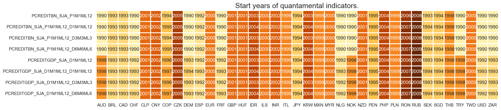
Real-time quantamental indicators of private credit expansion are available from the 1990s for most developed markets and some emerging markets. Most EM indicators, however, start in the early 2000s.
For the explanation of currency symbols, which are related to currency areas or countries for which categories are available, please view Appendix 1 .
xcatx = main
cidx = cids_exp

dfx = msm.reduce_df(df, xcats=xcatx, cids=cidx)
dfs = msm.check_startyears(dfx)
msm.visual_paneldates(dfs, size=(18, 4))

print("Last updated:", date.today())
Last updated: 2025-03-26
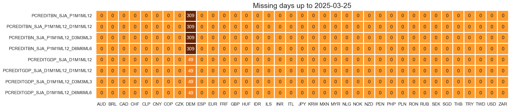
plot = msm.check_availability(
    df, xcats=xcatx, cids=cidx, start_size=(18, 2), start_years=False, start=start_date
)
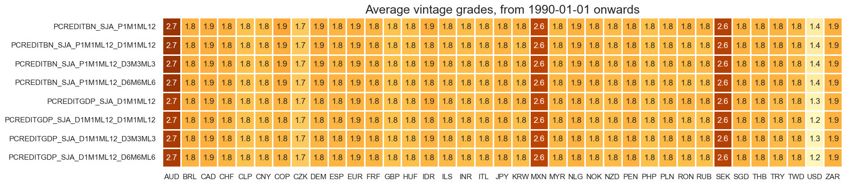
Average grades are currently quite mixed across countries and times, with USD the only cross-section with high grade vintages consistently available across indicators.
plot = msp.heatmap_grades(
    df,
    xcats=xcatx,
    cids=cidx,
    start=start_date,
    size=(18, 4),
    title=f"Average vintage grades, from {start_date} onwards",
)
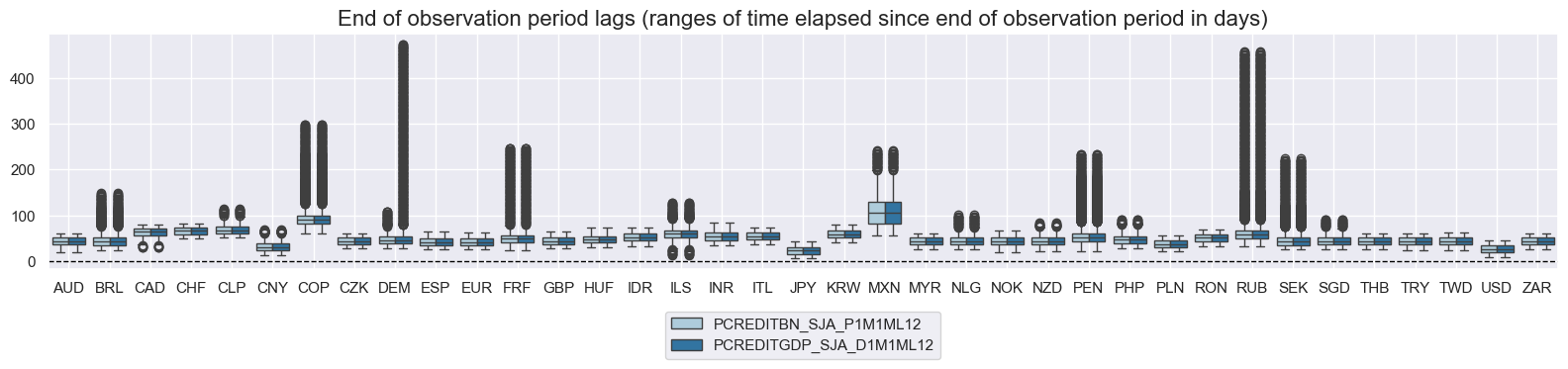
xcatx = main[:2]
msp.view_ranges(
df,
xcats=xcatx,
cids=cids_exp,
val="eop_lag",
title="End of observation period lags (ranges of time elapsed since end of observation period in days)",
start="2000-01-01",
kind="box",
size=(16, 4),
)
msp.view_ranges(
df,
xcats=xcatx,
cids=cids_exp,
val="mop_lag",
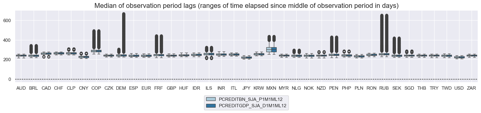
title="Median of observation period lags (ranges of time elapsed since middle of observation period in days)",
start="2000-01-01",
kind="box",
size=(16, 4),
)
History #
Nominal private credit growth #
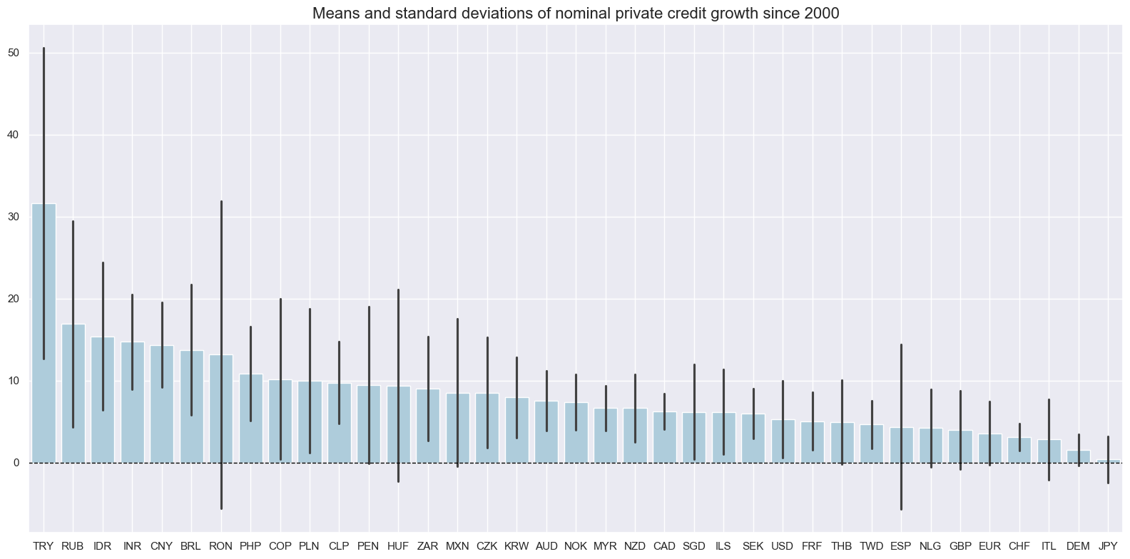
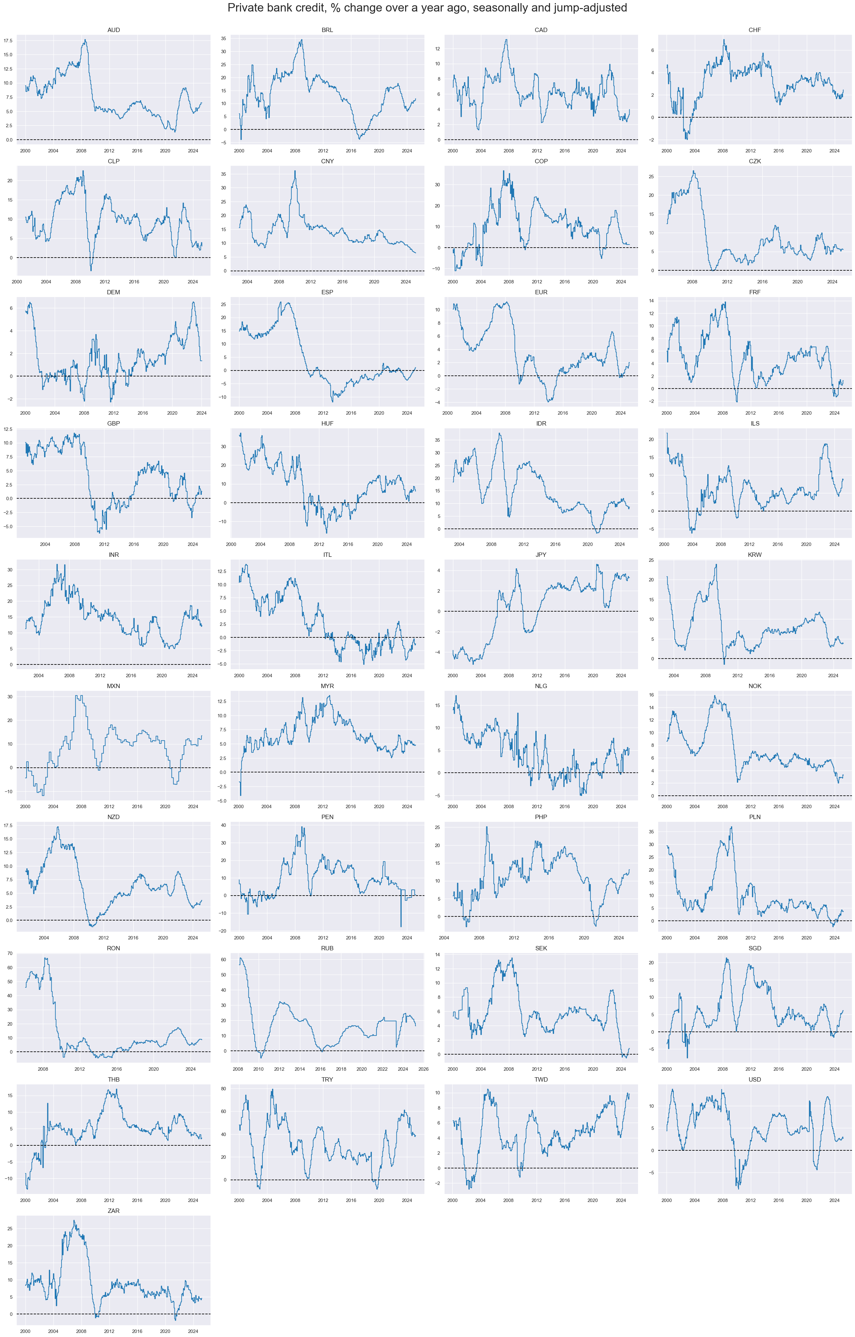
Long-term credit growth has been in a range of 5-15% for most countries. Across time, most countries have experienced pronounced fluctuations in private credit expansion, illustrating the importance of boom-bust patterns in credit cycles.
xcatx = ["PCREDITBN_SJA_P1M1ML12"]
cidx = cids_exp

msp.view_ranges(
    df,
    xcats=xcatx,
    cids=cidx,
    sort_cids_by="mean",
    title="Means and standard deviations of nominal private credit growth since 2000",
    kind="bar",
    start="2000-01-01",
    size=(16, 8),
)
xcatx = ["PCREDITBN_SJA_P1M1ML12"]
cidx = cids_exp

msp.view_timelines(
    df,
    xcats=xcatx,
    cids=cidx,
    start="2000-01-01",
    title="Private bank credit, % change over a year ago, seasonally and jump-adjusted",
    title_fontsize=27,
    ncol=4,
    same_y=False,
    size=(12, 7),
    all_xticks=True,
)
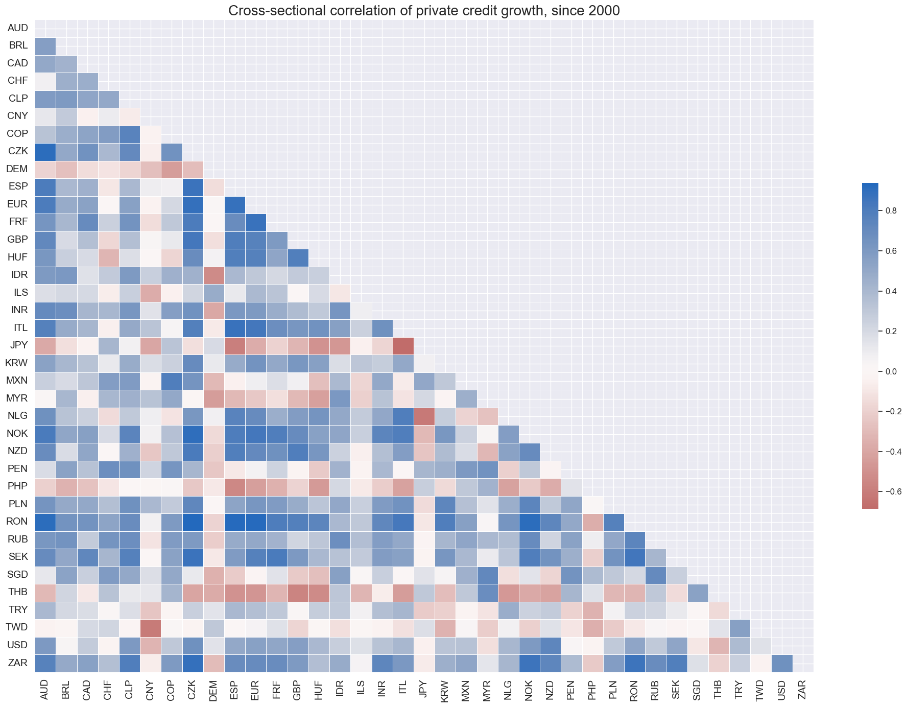
Correlations across currency areas have been mostly positive, with a small group of outliers. The outliers have been countries that experienced pronounced idiosyncratic credit cycles: China, Japan, the Philippines, Thailand, Taiwan, and Turkey.
msp.correl_matrix(
    df,
    xcats="PCREDITBN_SJA_P1M1ML12",
    cids=cids_exp,
    size=(20, 14),
    title="Cross-sectional correlation of private credit growth, since 2000",
)
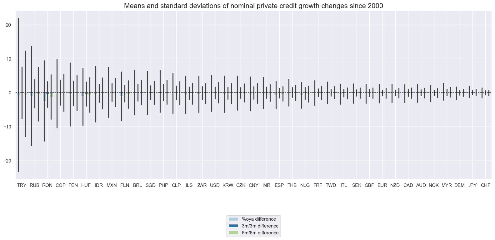
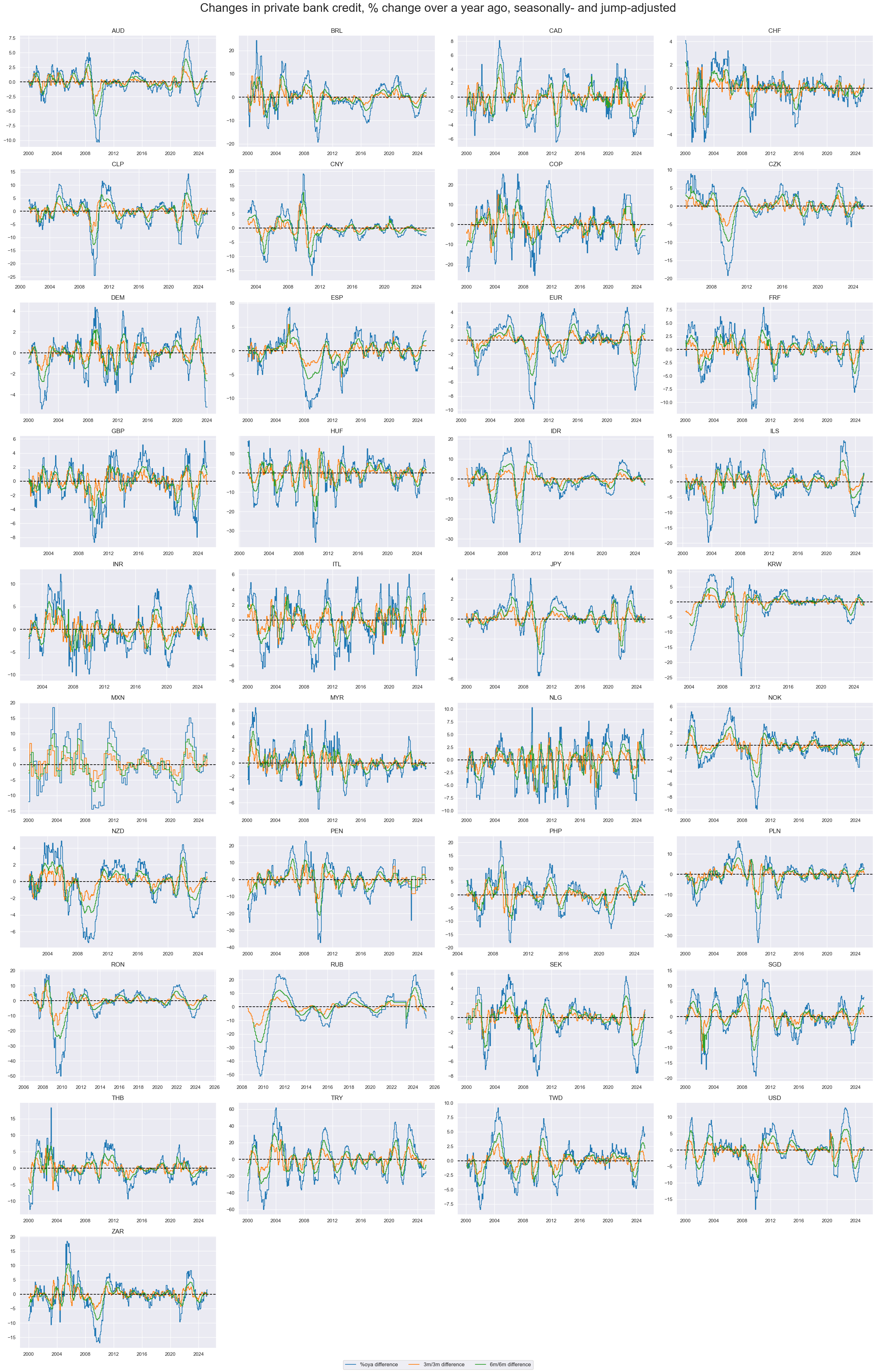
Changes in nominal private credit growth #
Mean changes for each cross-section have been small relative to their variance, for each of the three categories.
xcatx = [
    "PCREDITBN_SJA_P1M1ML12_D1M1ML12",
    "PCREDITBN_SJA_P1M1ML12_D3M3ML3",
    "PCREDITBN_SJA_P1M1ML12_D6M6ML6",
]
cidx = cids_exp

msp.view_ranges(
    df,
    xcats=xcatx,
    cids=cidx,
    sort_cids_by="std",
    start="2000-01-01",
    kind="bar",
    size=(16, 8),
    title="Means and standard deviations of nominal private credit growth changes since 2000",
    xcat_labels=["%oya difference", "3m/3m difference", "6m/6m difference"],
)
xcatx = [
    "PCREDITBN_SJA_P1M1ML12_D1M1ML12",
    "PCREDITBN_SJA_P1M1ML12_D3M3ML3",
    "PCREDITBN_SJA_P1M1ML12_D6M6ML6",
]
cidx = cids_exp

msp.view_timelines(
    df,
    xcats=xcatx,
    cids=cidx,
    start="2000-01-01",
    title="Changes in private bank credit, % change over a year ago, seasonally- and jump-adjusted",
    title_fontsize=27,
    ncol=4,
    same_y=False,
    size=(12, 10),
    all_xticks=True,
    xcat_labels=["%oya difference", "3m/3m difference", "6m/6m difference"],
)
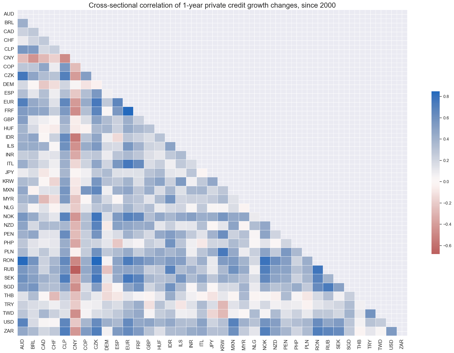
Cross-sectional correlations have generally been positive. China displays notable negative correlation with most other cross-sections in the panel. Thailand, Turkey and Taiwan also stand out with their idiosyncracies.
msp.correl_matrix(
    df,
    xcats="PCREDITBN_SJA_P1M1ML12_D1M1ML12",
    cids=cids_exp,
    size=(20, 14),
    title="Cross-sectional correlation of 1-year private credit growth changes, since 2000",
)
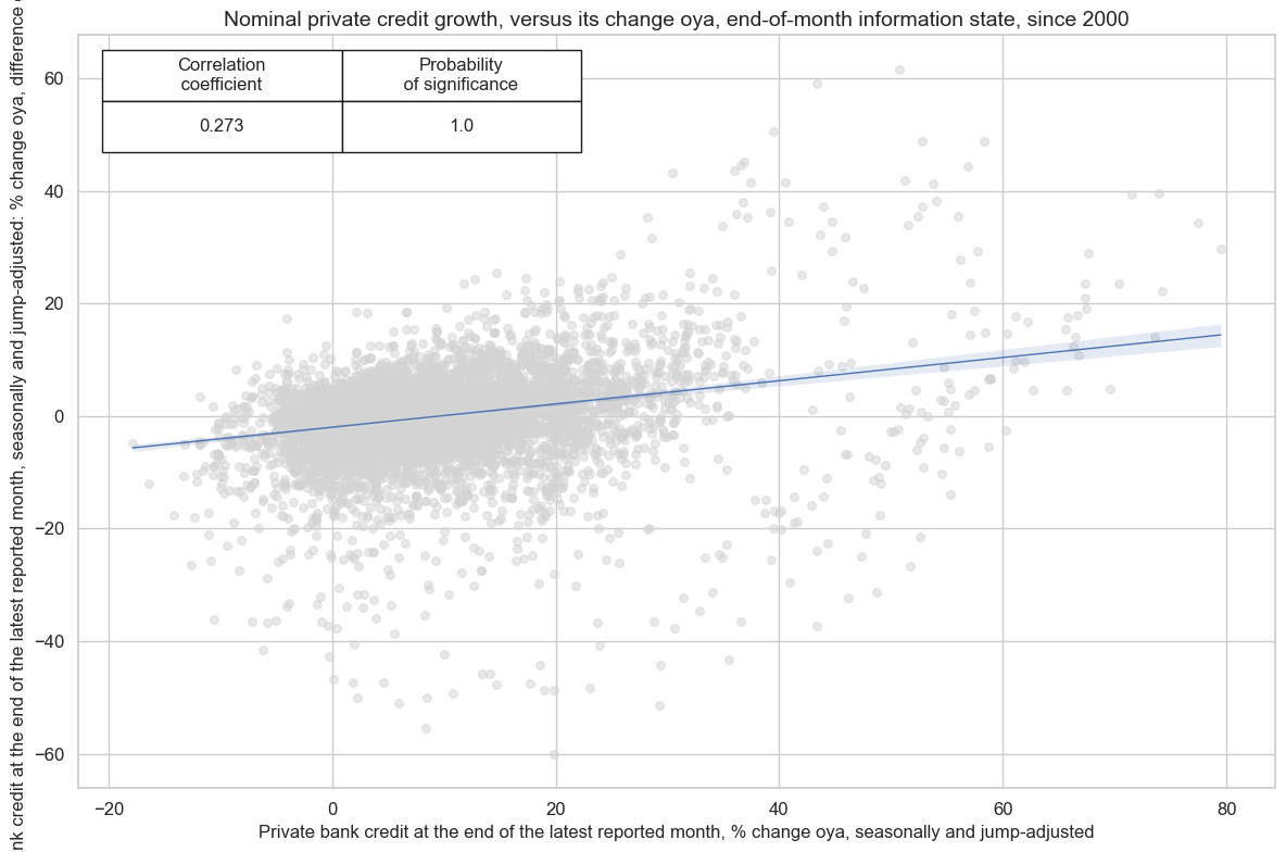
cidx=cids_exp

cr = msp.CategoryRelations(
    df,
    xcats=["PCREDITBN_SJA_P1M1ML12", "PCREDITBN_SJA_P1M1ML12_D1M1ML12"],
    cids=cidx,
    freq="M",
    lag=1,
    xcat_aggs=["last", "last"],
   # xcat_trims=[20,20],
    start="2000-01-01",
)

cr.reg_scatter(
        labels=False,
    coef_box="upper left",
    title = "Nominal private credit growth, versus its change oya, end-of-month information state, since 2000",
    xlab="Private bank credit at the end of the latest reported month, % change oya, seasonally and jump-adjusted",
    ylab="Private bank credit at the end of the latest reported month, seasonally and jump-adjusted: % change oya, difference oya (monthly)",
    prob_est="map"
)
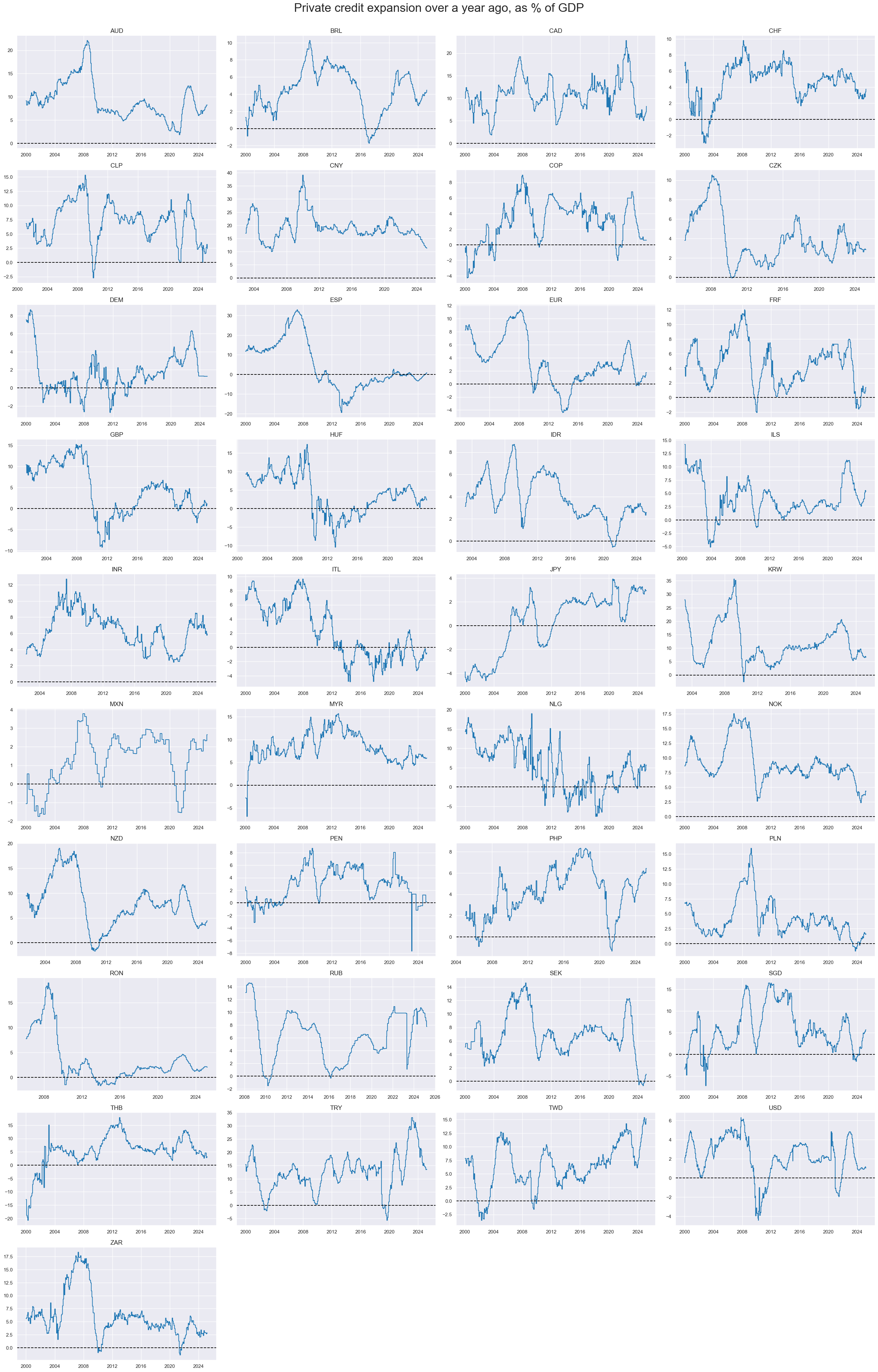
Private credit expansion as % of GDP #
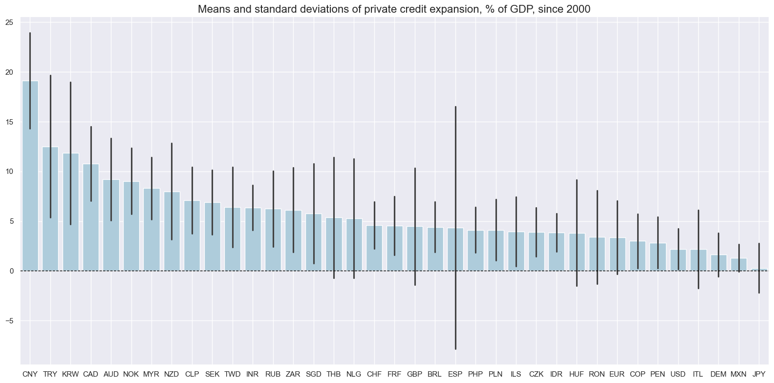
Unlike percent growth, credit growth in relation to GDP is strongly influenced by existing leverage. All other things equal, countries with larger financial systems post higher values and greater fluctuations. The order of countries in terms of magnitude of expansion is quite different from the order according to simple nominal credit growth.
xcatx = ["PCREDITGDP_SJA_D1M1ML12"]
cidx = cids_exp

msp.view_ranges(
    df,
    xcats=xcatx,
    cids=cidx,
    sort_cids_by="mean",
    start="2000-01-01",
    kind="bar",
    size=(16, 8),
    title="Means and standard deviations of private credit expansion, % of GDP, since 2000",
)
xcatx = ["PCREDITGDP_SJA_D1M1ML12"]
cidx = cids_exp

msp.view_timelines(
    df,
    xcats=xcatx,
    cids=cidx,
    start="2000-01-01",
    title="Private credit expansion over a year ago, as % of GDP",
    title_fontsize=27,
    ncol=4,
    same_y=False,
    size=(12, 7),
    all_xticks=True,
)
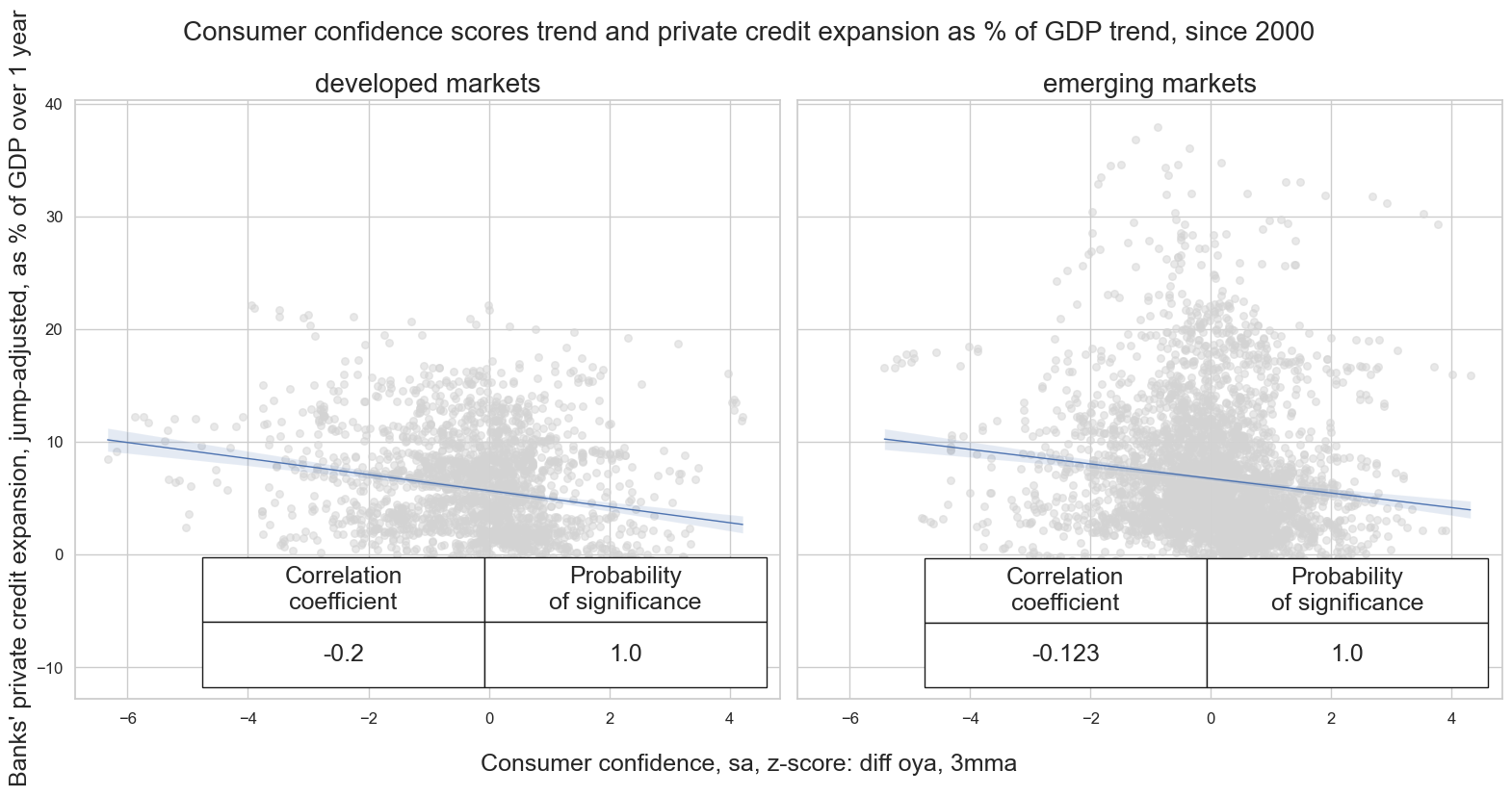
cidx = {
    "developed markets": list(set(cids_dmca) - {"CHF", "NZD"}),   # data not available for "CHF" and "NZD"
    "emerging markets": list(set(cids_em) - {"HKD", "PEN", "PHP", "RON", "RUB", "SGD", "ZAR"}),  # data not available for these currencies
}


cr = {}

sig = "CCSCORE_SA_3MMA_D1M1ML12"

for cid_name, cid_list in cidx.items():

    cr[f"cr_{cid_name}"] = msp.CategoryRelations(
        df,
        xcats=[sig, "PCREDITGDP_SJA_D1M1ML12"],
        cids=cid_list,
        freq="M",
        lag=0,
        xcat_aggs=["mean", "mean"],
       # blacklist=fxblack,
        start="2000-01-01",
        xcat_trims=[None, None]
    )

# Combine all CategoryRelations instances for plotting
all_cr_instances = [
    cr[f"cr_{cid_name}"]
    for cid_name in cidx.keys()
]

# Dynamically create subplot titles based on identifiers and market types
subplot_titles = [
    f"{cid_name}"  # Use the descriptive keys from cidx directly
    for cid_name in cidx.keys()
]

msv.multiple_reg_scatter(
    all_cr_instances,
    title="Consumer confidence scores trend and private credit expansion as % of GDP trend, since 2000",
    xlab="Consumer confidence, sa, z-score: diff oya, 3mma",
    ylab="Banks' private credit expansion, jump-adjusted, as % of GDP over 1 year",
    ncol=2,
    nrow=1,
    figsize=(16, 8),
    prob_est="map",
    coef_box="lower right",
    coef_box_size=(0.8, 4),
    coef_box_font_size=18,
    subplot_titles=subplot_titles,
    subplot_title_fontsize=20,
    label_fontsize=18,
)
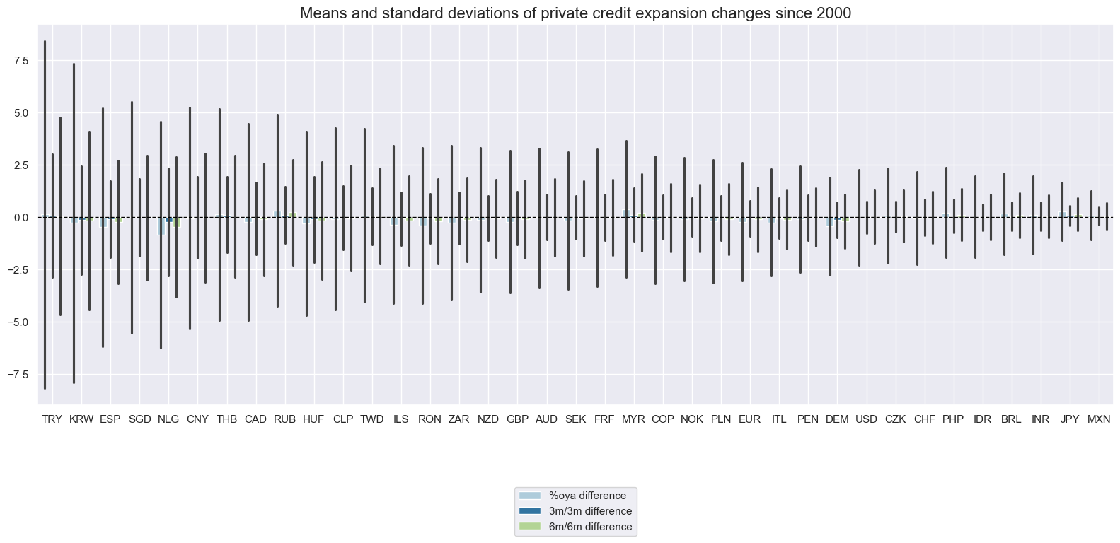
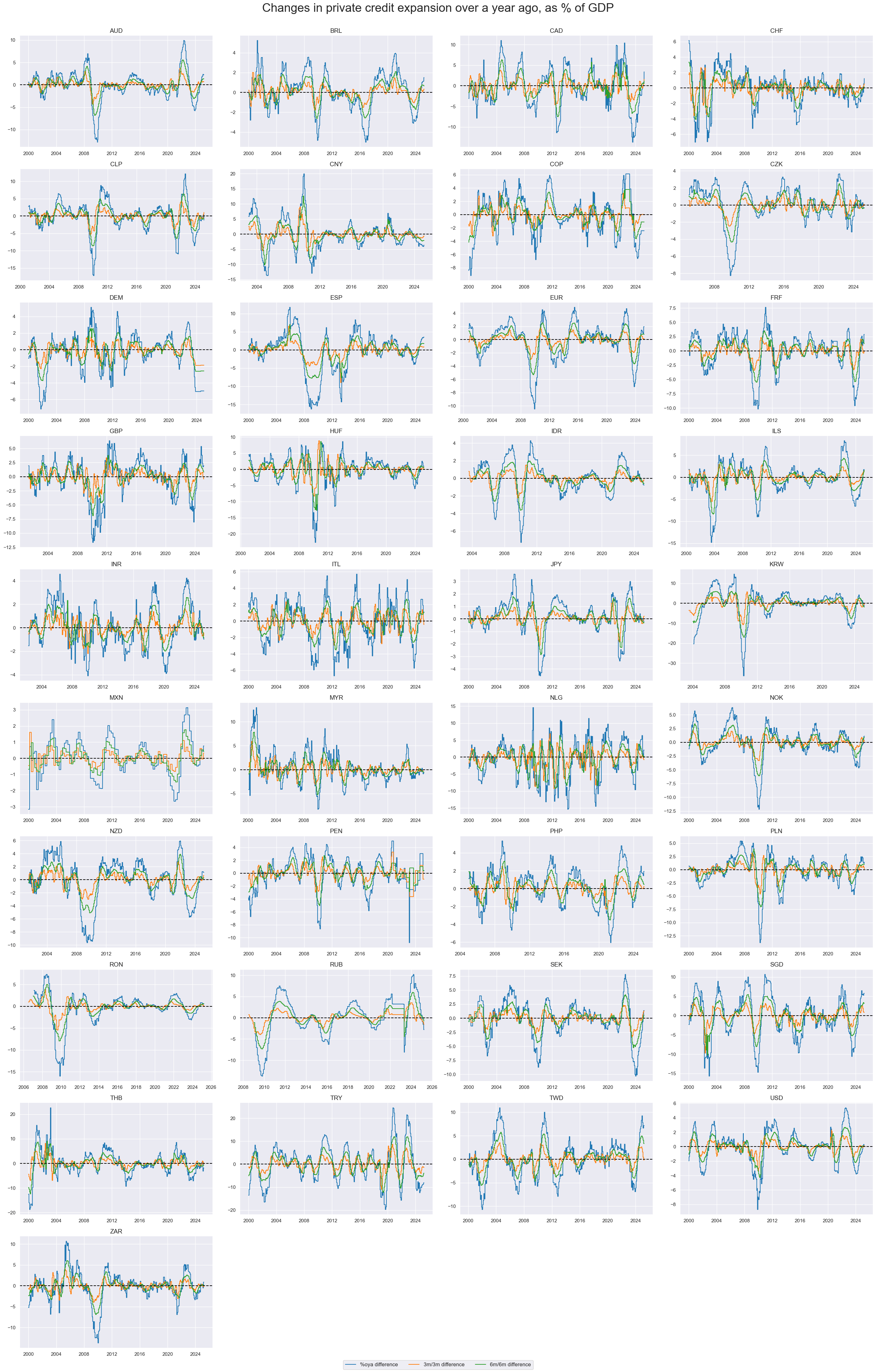
Changes in private credit expansion #
As previous, mean changes are generally small compared to their variances.
xcatx = [
    "PCREDITGDP_SJA_D1M1ML12_D1M1ML12",
    "PCREDITGDP_SJA_D1M1ML12_D3M3ML3",
    "PCREDITGDP_SJA_D1M1ML12_D6M6ML6",
]
cidx = cids_exp

msp.view_ranges(
    df,
    xcats=xcatx,
    cids=cidx,
    sort_cids_by="std",
    start="2000-01-01",
    kind="bar",
    size=(16, 8),
    title="Means and standard deviations of private credit expansion changes since 2000",
    xcat_labels=["%oya difference", "3m/3m difference", "6m/6m difference"]
)
xcatx = [
    "PCREDITGDP_SJA_D1M1ML12_D1M1ML12",
    "PCREDITGDP_SJA_D1M1ML12_D3M3ML3",
    "PCREDITGDP_SJA_D1M1ML12_D6M6ML6",
]
cidx = cids_exp

msp.view_timelines(
    df,
    xcats=xcatx,
    cids=cidx,
    start="2000-01-01",
    title="Changes in private credit expansion over a year ago, as % of GDP",
    title_fontsize=27,
    ncol=4,
    same_y=False,
    size=(12, 10),
    all_xticks=True,
    xcat_labels=["%oya difference", "3m/3m difference", "6m/6m difference"]
)
Importance #
Research links #
on credit expansion and equity returns
“Asset returns move predictably over the credit cycle. Using credit expansion in the nonfinancial corporate sector to capture the phase of the credit cycle, this paper shows that both equity and corporate bond returns decline as credit expansion accelerates.” Hang Bai
“…credit expansion a particularly strong predictor of lower bank equity returns when dividend yield is low…” M Baron and W Xiong
on credit expansion and currency returns
“… Rapid expansions in private credit are often, but not always, followed by recessions and financial crises … K Nueller & E Verner
“Global banks drive lending booms in local currency markets (explaining) how currency strength fuels rather than curbs financial expansion in small and emerging economies, leading to escalating dynamics.” Macrosynergy
“…private credit consistently affects economic growth… (in BRICS economies) “ “…only private credit shocks in India and China (IS) have any spillover effects on the growth of the other countries… “ N Samargandi & A Kutan
“A 145-year empirical analysis suggests that asset price surges are most dangerous when they are associated with rising financial leverage. The combination of housing price bubbles and credit booms has been the most detrimental of all.” Macrosynergy
Empirical clues #
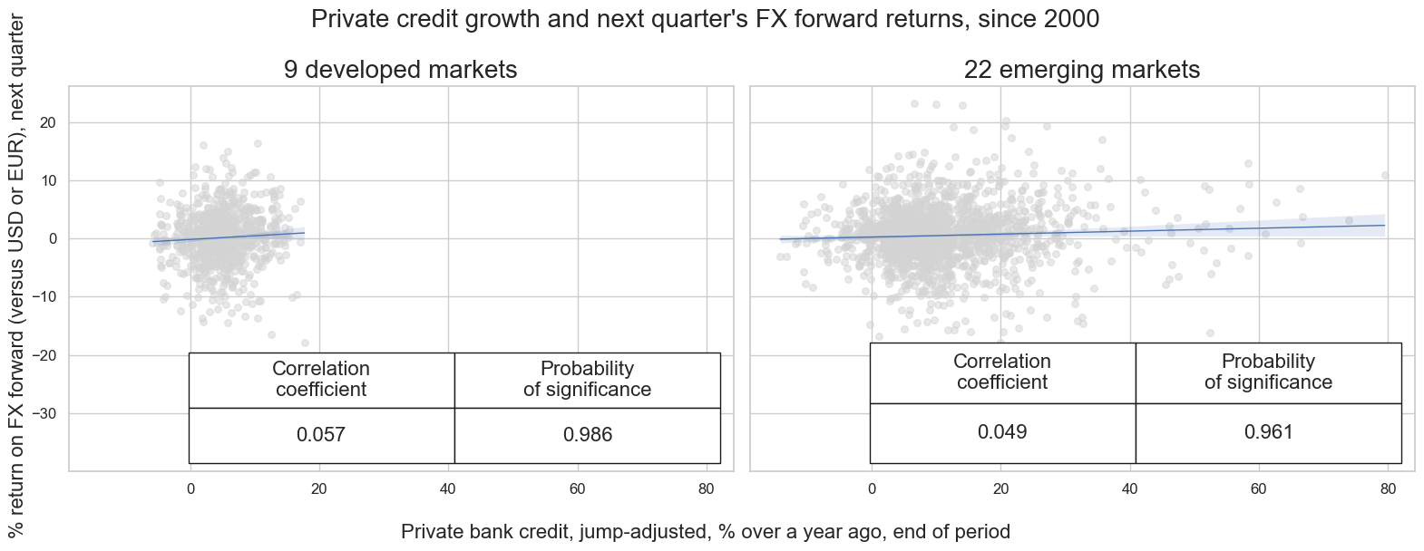
Private credit expansion as a predictor of FX returns #
Point-in-time information states of private credit growth have positively predicted FX forward returns at a monthly or quarterly frequency and for simple notional and volatility-targeted positions. The relation plausibly arises from the positive impact of credit expansion on local real interest rates. Predictive power has been stronger in the developed markets than for EM currencies.
dfx=df.copy()

dfb = dfx[dfx["xcat"].isin(["FXTARGETED_NSA", "FXUNTRADABLE_NSA"])].loc[
    :, ["cid", "xcat", "real_date", "value"]
]
dfba = (
    dfb.groupby(["cid", "real_date"])
    .aggregate(value=pd.NamedAgg(column="value", aggfunc="max"))
    .reset_index()
)
dfba["xcat"] = "FXBLACK"
fxblack = msp.make_blacklist(dfba, "FXBLACK")
cidx = {
    "9 developed markets": list(set(cids_dmca) - {"USD"}),
    "22 emerging markets": list(set(cids_em) - {"HKD"}),  # HKD not available
}

cr = {}

sig = "PCREDITBN_SJA_P1M1ML12"

for cid_name, cid_list in cidx.items():

    cr[f"cr_{cid_name}"] = msp.CategoryRelations(
        dfx,
        xcats=[sig, "FXXR_NSA"],
        cids=cid_list,
        freq="Q",
        lag=1,
        xcat_aggs=["last", "sum"],
        blacklist=fxblack,
        start="2000-01-01",
        xcat_trims=[None, None]
    )

# Combine all CategoryRelations instances for plotting
all_cr_instances = [
    cr[f"cr_{cid_name}"]
    for cid_name in cidx.keys()
]

# Dynamically create subplot titles
subplot_titles = [
    f"{cid_name}"  # Use the descriptive keys from cidx directly
    for cid_name in cidx.keys()
]


msv.multiple_reg_scatter(
    all_cr_instances,
    title="Private credit growth and next quarter's FX forward returns, since 2000",
    xlab="Private bank credit, jump-adjusted, % over a year ago, end of period",
    ylab="% return on FX forward (versus USD or EUR), next quarter",
    ncol=2,
    nrow=1,
    figsize=(16, 6),
    prob_est="map",
    coef_box="lower right",
    coef_box_size=(0.8, 4),
    coef_box_font_size=16,
    subplot_titles=subplot_titles,
    subplot_title_fontsize=20,
    label_fontsize=16,
)
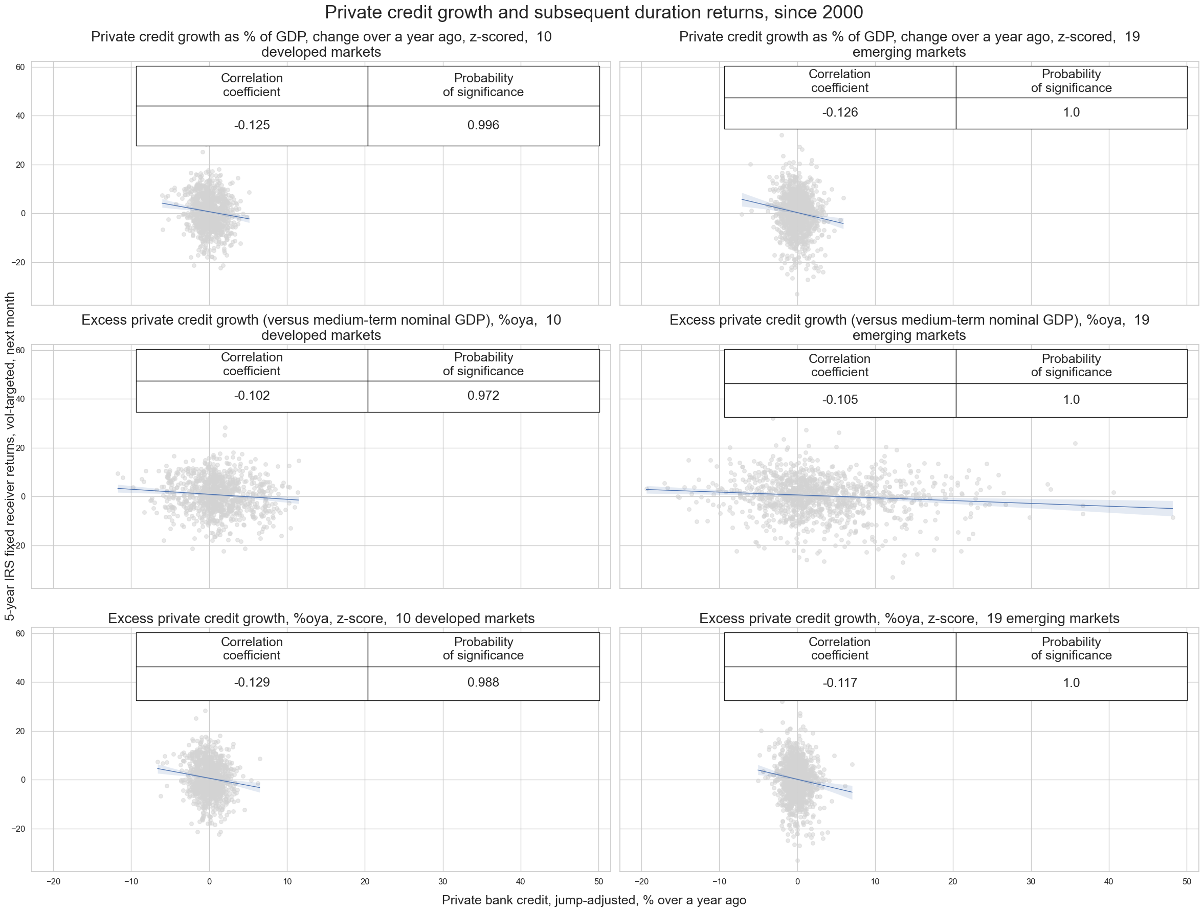
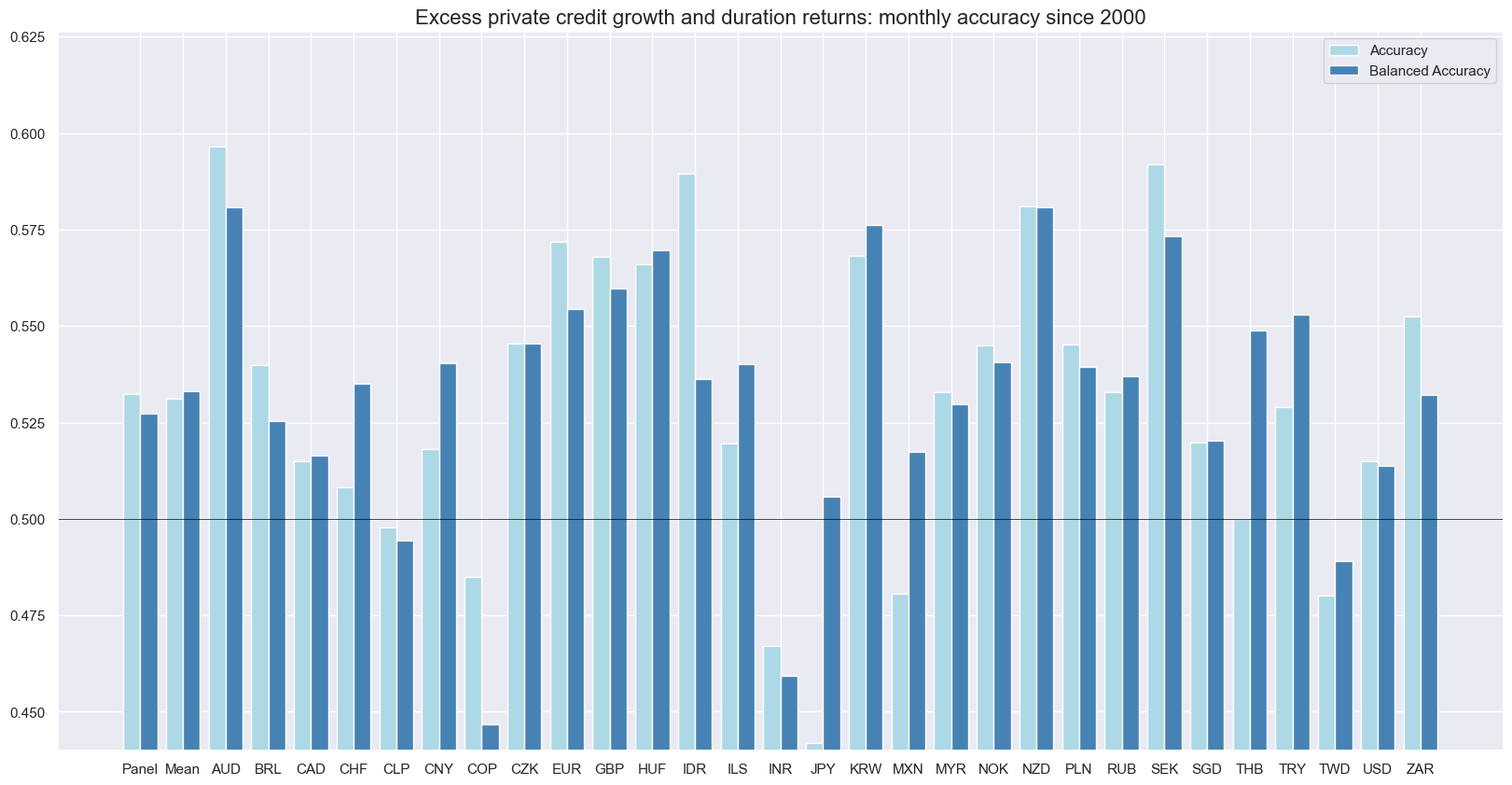
Private credit expansion as a predictor of IRS returns #
There is corresponding evidence of a negative correlation between private credit growth and subsequent IRS return, particularly when using the normalized version. Strong credit growth increases the probability of policy tightening and thus - all other things equal - bodes ill for long duration positions. Indeed, historically there has been a negative and signficant predictive relation between credit growth z-scores (normalized by country-specific means and standard deviation) and subsequent IRS receiever returns.
dfa = msp.panel_calculator(
    dfx,
    ["PCBASIS = INFTEFF_NSA + RGDP_SA_P1Q1QL4_20QMA"],
    cids=cids_exp,
)
dfx = msm.update_df(dfx, dfa)

pcgs = [
    "PCREDITBN_SJA_P1M1ML12",

]
for pcg in pcgs:
    calc_pcx = f"{pcg}vLTB = {pcg} - PCBASIS "
    dfa = msp.panel_calculator(dfx, calcs=[calc_pcx], cids=cids_exp)
    dfx = msm.update_df(dfx, dfa)
# Compute Zn scores
xcatx = ["PCREDITGDP_SJA_D1M1ML12", "PCREDITBN_SJA_P1M1ML12vLTB", "PCREDITBN_SJA_P1M1ML12"]
cidx = cids_exp

for xcat in xcatx:
    dfa = msp.make_zn_scores(
        dfx,
        cids=list(cidx),
        xcat=xcat,
        start="2000-01-01",
        est_freq="m",
        neutral="mean",
        # thresh=0,
        pan_weight=0,
    )
    dfx = msm.update_df(dfx, dfa)
xcatx_map = {"ZN": "PCREDITGDP_SJA_D1M1ML12ZN",
             "excess": "PCREDITBN_SJA_P1M1ML12vLTB",
             "excessZN": "PCREDITBN_SJA_P1M1ML12vLTBZN"}

cidx = {"10 developed markets": list(set(cids_dmca)),
        "19 emerging markets": list(set(cids_em) - set (["HKD", 'PEN', 'PHP', 'RON']))} # no data for these currencies

# Define xlab_dict with appropriate labels
xlab_dict = {
    "PCREDITGDP_SJA_D1M1ML12ZN": "Private credit growth as % of GDP, change over a year ago, z-scored, ",
    "PCREDITBN_SJA_P1M1ML12vLTB": "Excess private credit growth (versus medium-term nominal GDP), %oya, ",
    "PCREDITBN_SJA_P1M1ML12vLTBZN": "Excess private credit growth, %oya, z-score, "
}

cr = {}

# Iterate through the mapped signals and country groups
for identifier, sig in xcatx_map.items():
    for cid_name, cid_list in cidx.items():
        key = f"cr_{identifier}{cid_name}"  # Create keys like cr_ZN_dmca, cr_ZN_em, cr_dmca, cr_em
        cr[key] = msp.CategoryRelations(
            dfx,
            xcats=[sig, "DU05YXR_VT10"],
            cids=cid_list,
            freq="Q",
            lag=1,
            xcat_aggs=["last", "sum"],
            blacklist=fxblack,
            start="2000-01-01",
            xcat_trims=[None, None]
        )

# Combine all CategoryRelations instances for plotting
all_cr_instances = [
    cr[f"cr_{identifier}{cid_name}"]
    for identifier in xcatx_map.keys()
    for cid_name in cidx.keys()
]

# Dynamically create subplot titles based on identifiers and market types
subplot_titles = [
    f"{xlab_dict[xcatx_map[identifier]]} {cid_name}"
    for identifier in xcatx_map.keys()
    for cid_name in cidx.keys()
]

msv.multiple_reg_scatter(
        all_cr_instances,
        title="Private credit growth and subsequent duration returns, since 2000" ,
        title_fontsize=26,
        xlab="Private bank credit, jump-adjusted, % over a year ago",
        ylab="5-year IRS fixed receiver returns, vol-targeted, next month",
        ncol=2,
        nrow=3,
        figsize=(24, 18),
        prob_est="map",
        subplot_titles = subplot_titles,
        coef_box="upper right",
        coef_box_size=(0.8, 4),
        coef_box_font_size=18,
        subplot_title_fontsize=20,
        label_fontsize=18,
     )
cidx = msm.common_cids(dfx, xcats=xcatx)

xcatx = ["PCREDITBN_SJA_P1M1ML12vLTBZN", "DU05YXR_VT10"]
filtered_dfx = dfx[dfx['xcat'].isin(xcatx)]
scols = ["cid", "xcat", "real_date", "value"]
filtered_dfx = filtered_dfx[scols].copy().sort_values(["cid", "xcat", "real_date"])

srr = mss.SignalReturnRelations(
    filtered_dfx,
    cids=cidx,
    sigs="PCREDITBN_SJA_P1M1ML12vLTBZN",
    sig_neg=True,
    rets="DU05YXR_VT10",
    freqs="M",
    start="2000-01-01",
)

srr.accuracy_bars(
    type="cross_section",
    title="Excess private credit growth and duration returns: monthly accuracy since 2000",
    size=(20, 10),
    legend_pos="best",
)
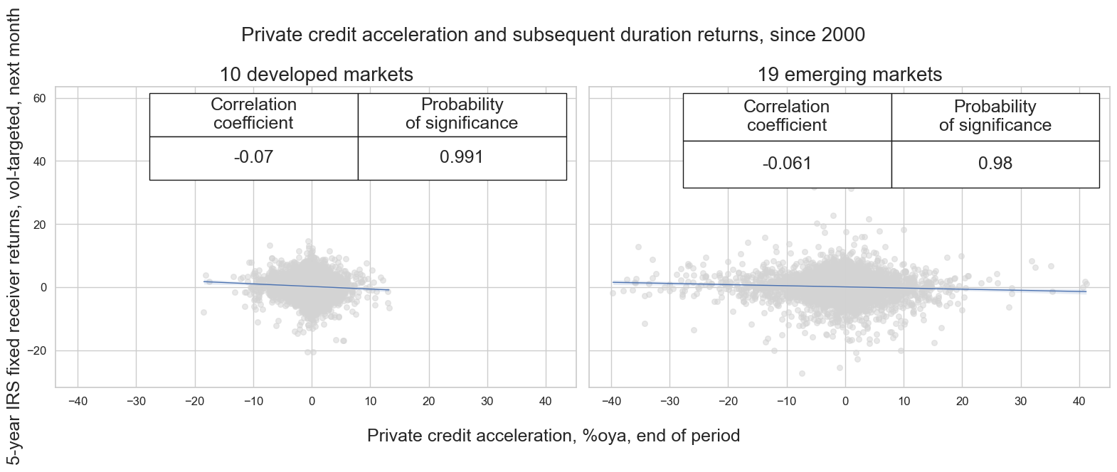
Private credit acceleration as a predictor of IRS returns #
Acceleration in private credit encourages central banks to lower interest rates, which should be detrimental to the IRS market.
# Annualize 3m/3m and 6m/6m private credit growth changes
dfa = msp.panel_calculator(
    df = dfx,
    calcs = [
        "PCREDITBN_SJA_P1M1ML12_D6M6ML6AR = PCREDITBN_SJA_P1M1ML12_D6M6ML6 * 2",
        "PCREDITBN_SJA_P1M1ML12_D3M3ML3AR = PCREDITBN_SJA_P1M1ML12_D3M3ML3 * 4",
    ],
    cids = cids_exp
)
dfx = msm.update_df(dfx, dfa)

# Create a private credit acceleration factor by averaging the three indicators
dfa = msp.linear_composite(
    df = dfx,
    xcats = [
        "PCREDITBN_SJA_P1M1ML12_D6M6ML6AR",
        "PCREDITBN_SJA_P1M1ML12_D3M3ML3AR",
        "PCREDITBN_SJA_P1M1ML12_D1M1ML12",
    ],
    cids = cids_exp,
    new_xcat="PCREDITACC"
)
dfx = msm.update_df(dfx, dfa)
cidx = {
    "10 developed markets": list(set(cids_dmca)),
    "19 emerging markets": list(set(cids_em) - set (["HKD", 'PEN', 'PHP', 'RON']))} # no data for these currencies


cr = {}

sig = "PCREDITACC"

for cid_name, cid_list in cidx.items():
    key = f"cr_{cid_name}"  # Create keys like cr_all, cr_em
    cr[key] = msp.CategoryRelations(
        dfx,
        xcats=[sig, "DU05YXR_VT10"],
        cids=cid_list,
        freq="M",
        lag=1,
        xcat_aggs=["last", "sum"],
        blacklist=fxblack,
        start="2000-01-01",
        xcat_trims=[None, None]
    )

# Combine all CategoryRelations instances for plotting
all_cr_instances = [
    cr[f"cr_{cid_name}"]
    for cid_name in cidx.keys()
]

# Dynamically create subplot titles based on market types
subplot_titles = [
    f"{cid_name}"
    for cid_name in cidx.keys()
]

# Call the plotting function
msv.multiple_reg_scatter(
    all_cr_instances,
    title="Private credit acceleration and subsequent duration returns, since 2000",
    xlab="Private credit acceleration, %oya, end of period",
    ylab="5-year IRS fixed receiver returns, vol-targeted, next month",
    ncol=2,
    nrow=1,
    figsize=(16, 6),
    prob_est="map",
    coef_box="upper right",
    coef_box_size=(0.8, 4),
    coef_box_font_size=18,
    subplot_titles=subplot_titles,
    subplot_title_fontsize=20,
    label_fontsize=18,
)
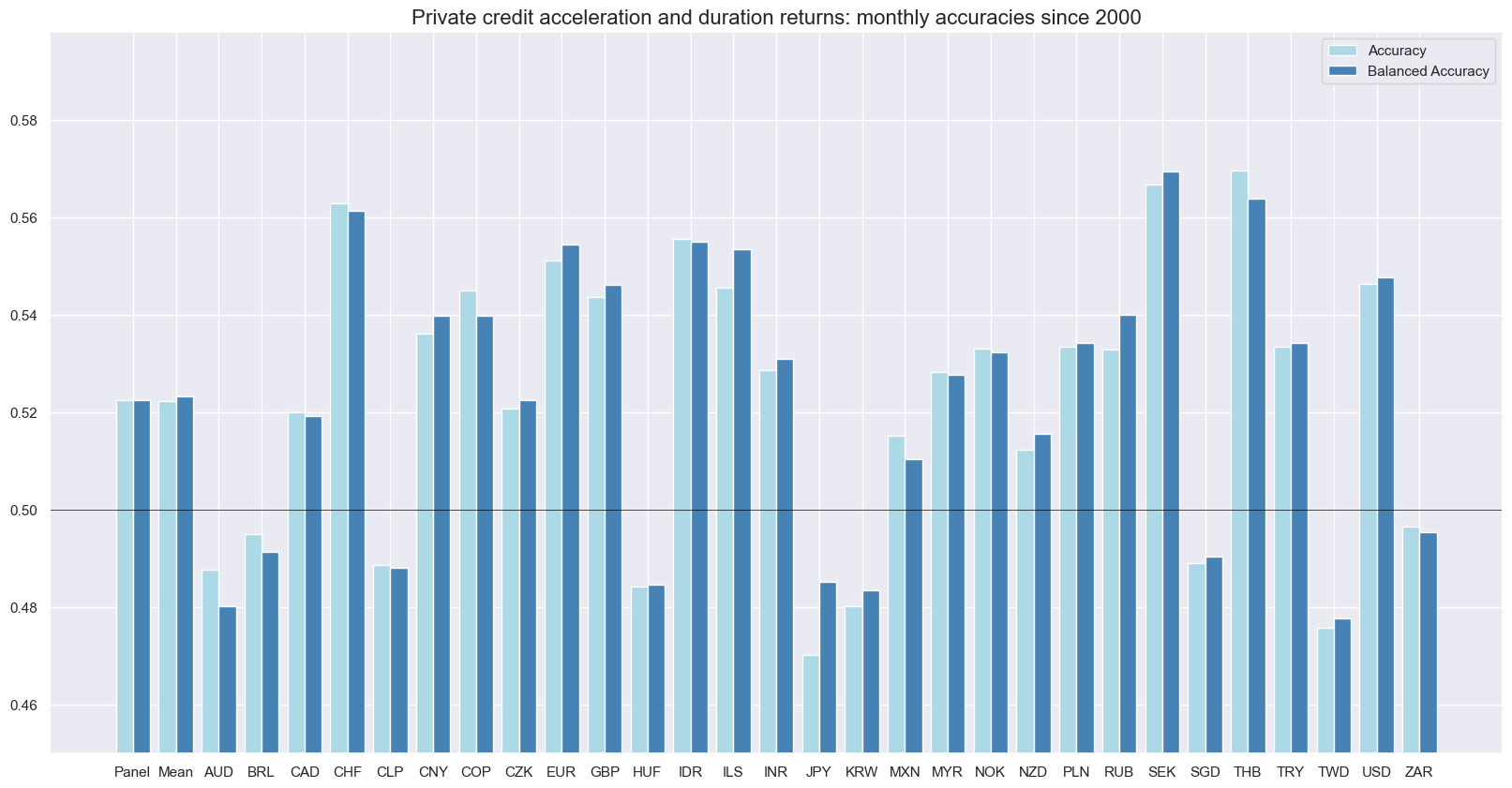
Accuracies for most currency areas are strong and the factor alone would have generated substantial PnL value over the last 25 years, albeit with some seasonality. A naive Sharpe in excess of 0.8 is realized.
srr = mss.SignalReturnRelations(
    dfx,
    cids=cids_exp,
    sigs="PCREDITACC",
    sig_neg=True,
    rets="DU05YXR_VT10",
    freqs="M",
    start="2000-01-01",
)

srr.accuracy_bars(
    title="Private credit acceleration and duration returns: monthly accuracies since 2000",
    size=(20, 10),
    legend_pos="best",
)
PnL generation has been material over multiple rebalancing frequencies. For convenience, we assume monthly rebalancing, but similar results hold for weekly and daily rebalancing.
pnl = msn.NaivePnL(
    df = dfx,
    ret = "DU05YXR_VT10",
    sigs = ["PCREDITACC"],
    cids = cids_exp,
    blacklist = fxblack,
    start = "2000-01-01"
)

pnl.make_long_pnl(vol_scale=10, label="LONG")

labels = {
    'LONG': 'Long only',
    'PNL_PCREDITACC_NEG': 'Private credit acceleration'
}

pnl.make_pnl(
    sig = "PCREDITACC",
    sig_op = "zn_score_cs",
    rebal_freq = "monthly",
    rebal_slip = 1,
    vol_scale = 10,
    neutral = "zero",
    thresh = 3,
    sig_neg = True
)

pnl.plot_pnls(
    pnl_cids=["ALL"],
    title="Naive PnLs of private credit acceleration, since 2000",
    title_fontsize=16,
    ylab="% of risk capital, for 10% annualized long-term vol, no compounding",
    start="01-01-2000",
    xcat_labels=labels,)

df_eval = pnl.evaluate_pnls(
    pnl_cats=["PNL_PCREDITACC_NEG"]+["LONG"],
)

df_eval = df_eval.rename(columns=labels)

df_eval = df_eval.style.format("{:.2f}").set_caption(
    f"Performance metrics of credit acceleration and long-only strategies, since 2000"
    ).set_table_styles(
    [{"selector": "caption", "props": [("text-align", "center"), ("font-weight", "bold"), ("font-size", "17px")]}
    ])

display(df_eval)
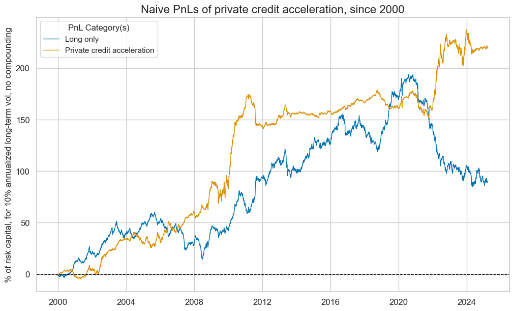
| xcat | Long only | Private credit acceleration |
|---|---|---|
| Return % | 3.51 | 8.71 |
| St. Dev. % | 10.00 | 10.00 |
| Sharpe Ratio | 0.35 | 0.87 |
| Sortino Ratio | 0.49 | 1.32 |
| Max 21-Day Draw % | -19.71 | -19.46 |
| Max 6-Month Draw % | -40.83 | -29.43 |
| Peak to Trough Draw % | -108.87 | -33.32 |
| Top 5% Monthly PnL Share | 1.63 | 0.89 |
| Traded Months | 303.00 | 303.00 |
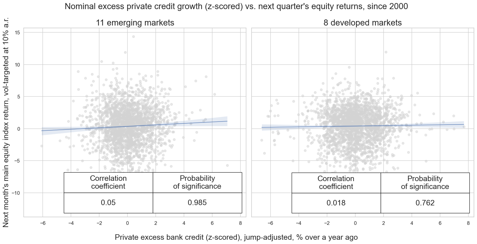
Private credit expansion as a predictor of equity returns #
There has been a positive predictive relation between information states of private credit growth and local-currency equity index futures returns at a monthly and quarterly frequency for emerging countries. This probably reflects the impact of capital inflows. The relation is much weaker for developed countries, presumably because the countervailing impact on monetary policy.
cidx = {"all": list(set(cids_eq) - set (["HKD"])),  # HKD has no data
        "em": list(set(cids_emeq)) }

cidx = {
    "11 emerging markets": cids_emeq,  # Similarly for cids_em
    "8 developed markets": cids_dmeq,  # Correct use of set with curly braces
}

cr = {}

sig = "PCREDITBN_SJA_P1M1ML12vLTBZN"

for cid_name, cid_list in cidx.items():
    key = f"cr_{cid_name}"  # Create keys like cr_all, cr_em
    cr[key] = msp.CategoryRelations(
        dfx,
        xcats=[sig, "EQXR_VT10"],
        cids=cid_list,
        freq="M",
        lag=1,
        xcat_aggs=["last", "sum"],
        blacklist=fxblack,
        start="2000-01-01",
        xcat_trims=[None, None]
    )

# Combine all CategoryRelations instances for plotting
all_cr_instances = [
    cr[f"cr_{cid_name}"]
    for cid_name in cidx.keys()
]

# Dynamically create subplot titles based on market types
subplot_titles = [
    f"{cid_name}"
    for cid_name in cidx.keys()
]

# Call the plotting function
msv.multiple_reg_scatter(
    all_cr_instances,
    title="Nominal excess private credit growth (z-scored) vs. next quarter's equity returns, since 2000",
    xlab="Private excess bank credit (z-scored), jump-adjusted, % over a year ago",
    ylab="Next month's main equity index return, vol-targeted at 10% a.r.",
    ncol=2,
    nrow=1,
    figsize=(16, 8),
    prob_est="map",
    coef_box="lower right",
    coef_box_size=(0.8, 4),
    coef_box_font_size=18,
    subplot_titles=subplot_titles,
    subplot_title_fontsize=20,
    label_fontsize=18,
)
PCREDITBN_SJA_P1M1ML12vLTBZN misses: ['HKD'].
EQXR_VT10 misses: ['ILS'].
EQXR_VT10 misses: ['NOK', 'NZD'].
Appendices #
Appendix 1: Seasonal and jump adjustment details #
Seasonal and jump adjustment are performed on the underlying data vintages, not on the quantamental indicator. This means that a collection of vintages for a particular economic concept, organised as a matrix with each column a vintage \(\boldsymbol{r}_{i}\) in increasing order of the associated release date, \(\left[ \boldsymbol{r}_{1},...,\boldsymbol{r}_{T} \right]\) is transformed to a new collection of vintages \(\left[ f(\boldsymbol{r}_{1}),...,f(\boldsymbol{r}_{T}) \right]\) through a function \(f\) performing seasonal and jump adjustment.
Seasonal adjustment is as follows:
-
The US Census X13 algorithm is applied to each vintage of private credit levels. The underlying econometric model is a seasonal ARIMA model leveraging a two-sided filter. The point-in-time principle is maintained by applying this to each vintage.
-
Should this fail, a classical seasonal-trend decomposition is applied to each vintage using the
statsmodelsfunctionseasonal_decompose, which decomposes a time series into trend, seasonality and error components. By removing the seasonal component based on this decomposition, the original vintage has been adjusted for seasonality.
Jump adjustment is applied to each seasonally-adjusted vintage as follows:
-
For each vintage, 1-year rolling mean and standard deviation time series are calculated. These are used to adjust for “spikes” and “breaks”.
-
First, we calculate the absolute difference between the vintage time series and its 1 year rolling mean, as well as a subsequent series of Booleans indicating whether or not this was greater than twice the 1-year rolling standard deviation. If so, this is termed a “jump”.
-
A “spike” is defined to be a “double jump”; a jump followed by a jump in the opposite direction. Based on the criterion for a jump, spikes are identified and replaced by the mean of the two samples that constitute the spike.
-
A “break” is a single jump, now that the spikes have been accounted for. These values are set to a np.NaN and replaced by the 1-year moving average.
Appendix 2: Floating rates #
In several countries, following the discontinuation of LIBOR, floating rates transitioned to Overnight Indexed Swaps (OIS). The table below also includes the new OIS rates in use and the date of each transition.
data = {
    "Indicator": [
        "AUD_PCREDITBN_SA", "BRL_PCREDITBN_NSA", "CAD_PCREDITBN_NSA", "CHF_PCREDITBN_NSA",
        "CLP_PCREDITBN_NSA", "CNY_PCREDITBN_NSA", "COP_PCREDITBN_NSA", "CZK_PCREDITBN_NSA",
        "DEM_PCREDITBN_NSA", "ESP_PCREDITBN_NSA", "EUR_PCREDITBN_NSA", "FRF_PCREDITBN_NSA",
        "GBP_PCREDITBN_NSA", "HUF_PCREDITBN_NSA", "IDR_PCREDITBN_NSA", "ILS_PCREDITBN_NSA",
        "INR_PCREDITBN_NSA", "ITL_PCREDITBN_NSA", "JPY_PCREDITBN_NSA", "KRW_PCREDITBN_NSA",
        "MXN_PCREDITBN_NSA", "MYR_PCREDITBN_NSA", "NLG_PCREDITBN_NSA", "NOK_PCREDITBN_NSA",
        "NZD_PCREDITBN_NSA", "PEN_PCREDITBN_NSA", "PHP_PCREDITBN_NSA", "PLN_PCREDITBN_NSA",
        "RON_PCREDITBN_NSA", "RUB_PCREDITBN_NSA", "SEK_PCREDITBN_NSA", "SGD_PCREDITBN_NSA",
        "THB_PCREDITBN_NSA", "TRY_PCREDITBN_NSA", "TWD_PCREDITBN_NSA", "USD_PCREDITBN_SA",
        "ZAR_PCREDITBN_NSA"
    ],
    "Underlying data": [
        "Total narrow credit lending excluding financial businesses", "Total credit operation outstanding",
        "Total credit liabilities of households and private non-financial corporations", "Total domestic loans",
        "Total domestic credit for the private sector from the banking sector", "Depository Corporations Survey - Domestic credit for non-financial sectors",
        "Gross domestic credit to the private sector", "Credit to other residents (non-government) (loans)",
        "Loans to domestic non-banks", "Domestic loans to other resident sectors",
        "Loans to other EA residents (excl. governments and MFIs)", "Domestic loans to the private sector",
        "Domestic loans to the private sector", "Loans to other residents", "Loans to the private sector",
        "Domestic private sector credit", "Domestic credit from commercial banks",
        "Other MFIs (excl. Central Bank) loans to other sectors", "Outstanding loans from domestic banks (excl. Shinkin Banks)",
        "Domestic loans to non-financial corporations and households", "Domestic loans to the private sector",
        "Total claims on the private sector", "Loan to EA residents (private sector)",
        "Domestic credit to non-financial corporations and households", "Loans to Housing & Personal Consumption and Businesses",
        "Total credit to the private sector", "Domestic claims to the private sector",
        "Total loans to domestic residents (non-MFI and non-government)", "Loans to the private sector",
        "Loans in local currency to individuals and organizations", "MFIs lending to households and non-financial corporations",
        "Domestic credit to the private sector", "Depository Corporations Survey - Domestic credit",
        "Loans to the private sector", "All banks loans outstanding", "Loan and leases in bank credit, all commercial banks",
        "Domestic private sector claims"
    ],
    "Source": [
        "Reserve Bank of Australia", "Central Bank of Brazil", "Statistics Canada", "National Bank of Switzerland",
        "Central Bank of Chile", "The People's Bank of China", "Central Bank of Colombia", "Czech National Bank",
        "Deutsche Bundesbank", "Bank of Spain", "ECB", "Banque de France", "Bank of England",
        "Central Bank of Hungary", "Bank Indonesia", "Bank of Israel", "Reserve Bank of India", "Banca d'Italia",
        "Bank of Japan", "Bank of Korea", "Bank of Mexico", "Central Bank of Malaysia",
        "Central Bank of Netherlands", "Statistics Norway", "Reserve Bank of New Zealand", "Central Reserve Bank of Peru",
        "Central Bank of the Philippines", "National Bank of Poland", "National Bank of Romania",
        "Central Bank of the Russian Federation", "Statistics Sweden", "Monetary Authority of Singapore",
        "Bank of Thailand", "Central Bank of the Republic of Türkiye", "Central Bank of Taiwan",
        "Federal Reserve", "Reserve Bank of South Africa"
    ]
}


summary = pd.DataFrame(data)
HTML(summary.to_html(index=False))
| Indicator | Underlying data | Source |
|---|---|---|
| AUD_PCREDITBN_SA | Total narrow credit lending excluding financial businesses | Reserve Bank of Australia |
| BRL_PCREDITBN_NSA | Total credit operation outstanding | Central Bank of Brazil |
| CAD_PCREDITBN_NSA | Total credit liabilities of households and private non-financial corporations | Statistics Canada |
| CHF_PCREDITBN_NSA | Total domestic loans | National Bank of Switzerland |
| CLP_PCREDITBN_NSA | Total domestic credit for the private sector from the banking sector | Central Bank of Chile |
| CNY_PCREDITBN_NSA | Depository Corporations Survey - Domestic credit for non-financial sectors | The People's Bank of China |
| COP_PCREDITBN_NSA | Gross domestic credit to the private sector | Central Bank of Colombia |
| CZK_PCREDITBN_NSA | Credit to other residents (non-government) (loans) | Czech National Bank |
| DEM_PCREDITBN_NSA | Loans to domestic non-banks | Deutsche Bundesbank |
| ESP_PCREDITBN_NSA | Domestic loans to other resident sectors | Bank of Spain |
| EUR_PCREDITBN_NSA | Loans to other EA residents (excl. governments and MFIs) | ECB |
| FRF_PCREDITBN_NSA | Domestic loans to the private sector | Banque de France |
| GBP_PCREDITBN_NSA | Domestic loans to the private sector | Bank of England |
| HUF_PCREDITBN_NSA | Loans to other residents | Central Bank of Hungary |
| IDR_PCREDITBN_NSA | Loans to the private sector | Bank Indonesia |
| ILS_PCREDITBN_NSA | Domestic private sector credit | Bank of Israel |
| INR_PCREDITBN_NSA | Domestic credit from commercial banks | Reserve Bank of India |
| ITL_PCREDITBN_NSA | Other MFIs (excl. Central Bank) loans to other sectors | Banca d'Italia |
| JPY_PCREDITBN_NSA | Outstanding loans from domestic banks (excl. Shinkin Banks) | Bank of Japan |
| KRW_PCREDITBN_NSA | Domestic loans to non-financial corporations and households | Bank of Korea |
| MXN_PCREDITBN_NSA | Domestic loans to the private sector | Bank of Mexico |
| MYR_PCREDITBN_NSA | Total claims on the private sector | Central Bank of Malaysia |
| NLG_PCREDITBN_NSA | Loan to EA residents (private sector) | Central Bank of Netherlands |
| NOK_PCREDITBN_NSA | Domestic credit to non-financial corporations and households | Statistics Norway |
| NZD_PCREDITBN_NSA | Loans to Housing & Personal Consumption and Businesses | Reserve Bank of New Zealand |
| PEN_PCREDITBN_NSA | Total credit to the private sector | Central Reserve Bank of Peru |
| PHP_PCREDITBN_NSA | Domestic claims to the private sector | Central Bank of the Philippines |
| PLN_PCREDITBN_NSA | Total loans to domestic residents (non-MFI and non-government) | National Bank of Poland |
| RON_PCREDITBN_NSA | Loans to the private sector | National Bank of Romania |
| RUB_PCREDITBN_NSA | Loans in local currency to individuals and organizations | Central Bank of the Russian Federation |
| SEK_PCREDITBN_NSA | MFIs lending to households and non-financial corporations | Statistics Sweden |
| SGD_PCREDITBN_NSA | Domestic credit to the private sector | Monetary Authority of Singapore |
| THB_PCREDITBN_NSA | Depository Corporations Survey - Domestic credit | Bank of Thailand |
| TRY_PCREDITBN_NSA | Loans to the private sector | Central Bank of the Republic of Türkiye |
| TWD_PCREDITBN_NSA | All banks loans outstanding | Central Bank of Taiwan |
| USD_PCREDITBN_SA | Loan and leases in bank credit, all commercial banks | Federal Reserve |
| ZAR_PCREDITBN_NSA | Domestic private sector claims | Reserve Bank of South Africa |
Appendix 3: Currency symbols #
The word ‘cross-section’ refers to currencies, currency areas or economic areas. In alphabetical order, these are AUD (Australian dollar), BRL (Brazilian real), CAD (Canadian dollar), CHF (Swiss franc), CLP (Chilean peso), CNY (Chinese yuan renminbi), COP (Colombian peso), CZK (Czech Republic koruna), DEM (German mark), ESP (Spanish peseta), EUR (Euro), FRF (French franc), GBP (British pound), HKD (Hong Kong dollar), HUF (Hungarian forint), IDR (Indonesian rupiah), ITL (Italian lira), JPY (Japanese yen), KRW (Korean won), MXN (Mexican peso), MYR (Malaysian ringgit), NLG (Dutch guilder), NOK (Norwegian krone), NZD (New Zealand dollar), PEN (Peruvian sol), PHP (Phillipine peso), PLN (Polish zloty), RON (Romanian leu), RUB (Russian ruble), SEK (Swedish krona), SGD (Singaporean dollar), THB (Thai baht), TRY (Turkish lira), TWD (Taiwanese dollar), USD (U.S. dollar), ZAR (South African rand).