Terms-of-trade #
This category group contains approximate dynamics of terms-of-trade. Currently, it is based on two main types. The first type, commodity-based terms of trade, uses commodity trade and price data alone, and can be consistently updated in real time at a daily frequency. The second type, mixed terms of trade, uses (a) low-frequency broad external trade data to capture medium-term dynamics and (b) daily commodity-based terms-of-trade to estimate recent and intermittent dynamics.
Generally, commodity terms-of-trade dynamics are ratios of approximate export and import price dynamics, whereby the latter are calculated on a daily basis based on concurrent vintages of commodity prices (in USD), commodity trade shares, and (as a non-commodity tradable USD goods’ price proxy) the U.S. core producer price index. There are two key differences between the JPMaQS commodities-based terms-of-trade series and those of other providers, beyond a set of more subtle methodological differences:
-
First, JPMaQS series are point-in-time, always using the latest available commodity trade weights and producer prices.
-
Second, while other externally available terms-of-trade proxy implicitly assumes stable non-commodity prices (effectively biasing terms-of-trade proxy in favor of commodity exporters), the JPMaQS proxy assumes that non-commodity export and import prices have grown in line with core PPI.
Commodity-based terms-of-trade dynamics #
Ticker : CTOT_NSA_PI / CTOT_NSA_P1M1ML12 / CTOT_NSA_P1W4WL1 / CTOT_NSA_P1M12ML1 / CTOT_NSA_P1M60ML1
Label : Commodities terms-of-trade, % change: since inception / latest month over a year ago / latest week over the previous 4 weeks / latest month over the previous 12 months / latest month over the previous 5 years
Definition : Commodities-based terms-of-trade, % change: since inception / latest month average (21 trading days) over the same month a year ago / latest week (5 trading days) over previous 4 weeks average / latest month average (21 trading days) over previous year average (261-trading days period) / latest month average (21 trading days) over previous 5 years average (1305-trading days period)
Notes :
-
Terms-of-trade dynamics are based on ratios of approximate export and import price dynamics, whereby the latter are calculated on a daily basis based on concurrent vintages of commodity prices (in USD), commodity trade shares, and (as a non-commodity tradable USD goods’ price proxy) the U.S. core producer price index. Export and import price dynamics are collected as ratios of latest price index divided by index at base period. For the exact calculation of commodity price-based export and import price indices see Appendix 1 .
-
The underlying vintages of all categories are based on commodity trade shares and related prices of liquidly-traded commodity contracts. Since the range of traded contracts has broadened overtime, so has the range of commodities that is used for the index. For example, for 1995, the number of usable contracts was 35. By 2005, it had grown to 44 and by 2015 to 55, which also marked the number contracts in use at the launch of this quantamental category in 2023. For details, see the bottom of Appendix 3 .
-
CTOT_NSA_PIis calculated based on the ratio of the export price index relative to inception divided by the import price index relative to inception, based on the concurrent vintage. The percent change is this ratio minus 1 and times 100. Since the change to inception is always based on the latest concurrent vintage (point-in-time), daily changes can reflect actual terms-of-trade alterations as well as revisions. However, since the actual terms-of-trade changes are very dominant, this category can (and inevitably will) be used as a proxy of a daily terms-of-trade index. Strictly speaking, there is no such thing as a single point-in-time terms-of-trade series, but a vintage matrix, i.e. a collection of updating terms-of-trade series. -
CTOT_NSA_P1M1ML12is calculated based on the ratio of (i) the export price index average of the latest month relative to the export price index average of the same month a year ago divided by (ii) the import price index average of the latest month relative to the import price index average of the same month a year ago, based on the concurrent vintage. The percent change is this ratio minus 1 and times 100. -
CTOT_NSA_P1W4WL1is calculated based on the ratio of (i) the export price index average of the latest week relative to the export price index average of the previous 4 weeks divided by (ii) the import price index average of the latest week relative to the import price index average of the previous 4 weeks, based on the concurrent vintage. The percent change is this ratio minus 1 and times 100. -
CTOT_NSA_P1M12ML1is calculated based on the ratio of (i) the export price index average of the latest month relative to export price index average of the previous 12 months divided by (ii) the import price index average of the latest month relative to the import price index average of the previous 12 months, based on the concurrent vintage. The percent change is this ratio minus 1 and times 100. -
CTOT_NSA_P1M60ML1is calculated based on the ratio of (i) the export price index average of the latest month relative to the export price index average of the previous 60 months divided by (ii) the import price index average of the latest month relative to the import price index average of the previous 60 months, based on the concurrent vintage. The percent change is this ratio minus 1 and times 100. -
Important : Percent changes of terms-of-trade are not symmetric but skewed to the high side. If only the export price index rises by 100%, the terms-of-trade change will be 100%. If only the import price index rises 100%, the terms of trade change will be 50%. If trading strategies and related research require symmetry, a logarithmic value of the implied change index or separate consideration of export and import price dynamics (see categories below) are more appropriate.
Mixed terms-of-trade dynamics #
Ticker : MTOT_NSA_PI / MTOT_NSA_P1M1ML12 / MTOT_NSA_P1W4WL1 / MTOT_NSA_P1M12ML1 / MTOT_NSA_P1M60ML1
Label : Mixed terms-of-trade, % change: since inception / latest month over a year ago / latest week over the previous 4 weeks / latest month over the previous 12 months / latest month over the previous 5 years
Definition : Combination of broad and commodity-based terms-of-trade, % change: since inception / latest month average (21 trading days) over the same month a year ago / latest week (5 trading days) over previous 4 weeks average / latest month average (21 trading days) over previous year average (261-trading days period) / latest month average (21 trading days) over previous 5 years average (1305-trading days period)
Notes :
-
Mixed terms-of-trade indicators are based on composite vintages. These vintages include actual broad export and import prices indices and, when these are not available, commodity-based indices. Since broad terms-of-trade are typically published at lower frequencies and with much longer lags, the commodity terms-of-trade are effectively used to predict and interpolate the broader series. For details on the methodology see Appendix 2 .
-
Broad export and import price indices are based on all traded items’ prices. Unlike commodity-based series, which are daily, the broad indices are released at annual or quarterly or monthly frequencies. For data reference see Appendix 4 .
-
Some countries (China, Hungary, Poland, Russia) do not publish broad export and import price indices, but only their percent changes over a year ago. In this case, we approximate the daily price levels of the first year in each vintage with the commodity indices and augment subsequently with the reported growth rates. This can result in artificial seasonality. Hence, short-term changes of these indicators should be regarded as rough proxies only.
-
Broad terms-of-trade can be subject to seasonality. Therefore, short-term changes of mixed terms-of-trade are subject to more noise around actual trends than medium-term changes.
-
MTOT_NSA_PIis calculated based on the ratio of the export price index relative to inception divided by import price index relative to inception, based on the concurrent vintage. The percent change is this ratio minus 1 and times 100. Since the change to inception is always based on the latest concurrent vintage (point-in-time), daily changes can reflect actual terms-of-trade alterations as well as revisions. In particular, releases of broad terms-of-trades can significantly alter the series. Hence, unlike in the case of commodity-based indices, this % change since inception should not be used as a proxy of a daily index. In the case of mixed terms-of-trades, revisions do play a great role and hence historical dynamics should always consider vintages. -
MTOT_NSA_P1M1ML12is calculated based on the ratio of (i) the mixed export price index average of the latest month relative to the mixed export price index average of the same month a year ago divided by (ii) the mixed import price index average of the latest month relative to the mixed import price index average of the same month a year ago, based on the concurrent vintage. The percent change is this ratio minus 1 and times 100. -
MTOT_NSA_P1M12ML1is calculated based on the ratio of (i) the mixed export price index average of the latest month relative to the mixed export price index average of the previous 12 months divided by (ii) the mixed import price index average of the latest month relative to the mixed import price index average of the previous 12 months, based on the concurrent vintage. The percent change is this ratio minus 1 and times 100. -
MTOT_NSA_P1M60ML1is calculated based on the ratio of (i) the mixed export price index average of the latest month relative to the mixed export price index average of the previous 60 months divided by (ii) the mixed import price index average of the latest month relative to the mixed import price index average of the previous 60 months, based on the concurrent vintage. The percent change is this ratio minus 1 and times 100. -
Important : Percent changes of mixed terms-of-trade are not symmetric but skewed to the high side. If only the export price index rises by 100%, the terms-of-trade change will be 100%. If only the import price index rises by 100%, the terms of trade change will be 50%. If trading strategies and related research require symmetry, a logarithmic value of the implied change index or separate consideration of export and import price dynamics (see categories below) are more appropriate.
Commodity-based export price dynamics #
Ticker : CXPI_NSA_PI / CXPI_NSA_P1M1ML12 / CXPI_NSA_P1W4WL1 / CXPI_NSA_P1M12ML1 / CXPI_NSA_P1M60ML1
Label : Commodities export price index, % change: since inception / latest month over a year ago / latest week over the previous 4 weeks / latest month over the previous 12 months / latest month over the previous 5 years
Definition : Commodities export price index, % change: since inception / latest month average (21 trading days) over the same month a year ago / atest week (5 trading days) over previous 4 weeks average / latest month average (21 trading days) over previous year average (261-trading days period) / latest month average (21 trading days) over previous 5 years average (1305-trading days period)
Notes :
-
All commodities export price index dynamics are based on concurrent vintages of commodity prices (in USD), commodity export trade shares, and (as a non-commodity tradable USD goods’ price proxy) the U.S. core producer price index.
-
The calculation of commodity price-based export and import price indices uses over 50 commodity categories. For details of the formulas used, see Appendix 1 and for details of the data used, see Appendix 3 .
Commodity-based import price dynamics #
Ticker : CMPI_NSA_PI / CMPI_NSA_P1M1ML12 / CMPI_NSA_P1W4WL1 / CMPI_NSA_P1M12ML1 / CMPI_NSA_P1M60ML1
Label : Commodities import price index, % change: since inception / latest month over a year ago / latest week over the previous 4 weeks / latest month over the previous 12 months / latest month over the previous 5 years
Definition : Commodities import price index, % change: since inception / latest month average (21 trading days) over the same month a year ago / latest week (5 trading days) over previous 4 weeks average / latest month average (21 trading days) over previous year average (261-trading days period) / latest month average (21 trading days) over previous 5 years average (1305-trading days period)
Notes :
-
All commodities import price index dynamics are based on concurrent vintages of commodity prices (in USD), commodity import trade shares, and (as a non-commodity tradable USD goods’ price proxy) the U.S. core producer price index.
-
The calculation of commodity price-based export and import price indices uses over 50 commodity categories. For details of the formulas used, see Appendix 1 and for details of the data used, see Appendix 3 .
Imports #
Only the standard Python data science packages and the specialized
macrosynergy
package are needed.
import os
import pandas as pd

import macrosynergy.management as msm
import macrosynergy.panel as msp
import macrosynergy.visuals as msv

from macrosynergy.download import JPMaQSDownload

from timeit import default_timer as timer
from datetime import timedelta, date

import warnings

warnings.simplefilter("ignore")
The
JPMaQS
indicators we consider are downloaded using the J.P. Morgan Dataquery API interface within the
macrosynergy
package. This is done by specifying
ticker strings
, formed by appending an indicator category code
<category>
to a currency area code
<cross_section>
. These constitute the main part of a full quantamental indicator ticker, taking the form
DB(JPMAQS,<cross_section>_<category>,<info>)
, where
<info>
denotes the time series of information for the given cross-section and category. The following types of information are available:
-
valuegiving the latest available values for the indicator -
eop_lagreferring to days elapsed since the end of the observation period -
mop_lagreferring to the number of days elapsed since the mean observation period -
gradedenoting a grade of the observation, giving a metric of real time information quality.
After instantiating the
JPMaQSDownload
class within the
macrosynergy.download
module, one can use the
download(tickers,start_date,metrics)
method to easily download the necessary data, where
tickers
is an array of ticker strings,
start_date
is the first collection date to be considered and
metrics
is an array comprising the times series information to be downloaded.
# Cross-sections of interest

cids_dmca = [
    "AUD",
    "CAD",
    "CHF",
    "EUR",
    "GBP",
    "JPY",
    "NOK",
    "NZD",
    "SEK",
    "USD",
]  # DM currency areas
cids_dmec = ["DEM", "ESP", "FRF", "ITL", "NLG"]  # DM euro area countries
cids_latm = ["BRL", "COP", "CLP", "MXN", "PEN"]  # Latam countries
cids_emea = ["CZK", "HUF", "ILS", "PLN", "RON", "RUB", "TRY", "ZAR"]  # EMEA countries
cids_emas = [
    "CNY",
    "HKD",
    "IDR",
    "INR",
    "KRW",
    "MYR",
    "PHP",
    "SGD",
    "THB",
    "TWD",
]  # EM Asia countries

cids_dm = cids_dmca + cids_dmec
cids_em = cids_latm + cids_emea + cids_emas


# for FX analysis

cids_dmfx =  ["AUD", "CAD", "CHF", "GBP", "NOK", "NZD", "SEK", "JPY"]
cids_emfx = ["BRL", "COP", "CLP", "MXN", "PEN", "CZK", "HUF",
    "ILS", "PLN", "RON", "RUB", "TRY", "ZAR", "IDR",
    "INR", "KRW", "MYR", "PHP", "THB", "TWD"]
cids_fx = cids_dmfx + cids_emfx

cids_eur = ["CHF", "CZK", "HUF", "NOK", "PLN", "RON", "SEK"]  # trading against EUR
cids_eud = ["GBP", "RUB", "TRY"]  # trading against EUR and USD
cids_usd = list(set(cids_fx) - set(cids_eur + cids_eud))

# for equity analysis
cids_dmeq = ["AUD", "CAD", "CHF", "EUR", "GBP", "JPY", "SEK", "USD"]
cids_emeq = ["CNY", "HKD", "INR", "KRW", "MYR", "SGD", "THB", "TWD", "BRL", "TRY", "ZAR", "MXN", "PLN"]
cids_eq = cids_dmeq + cids_emeq

cids = sorted(cids_dm + cids_em)
exps = [
    "CXPI_NSA_PI",
    "CXPI_NSA_P1M1ML12",
    "CXPI_NSA_P1W4WL1",
    "CXPI_NSA_P1M12ML1",
    "CXPI_NSA_P1M60ML1",
]
imps = [
    "CMPI_NSA_PI",
    "CMPI_NSA_P1M1ML12",
    "CMPI_NSA_P1W4WL1",
    "CMPI_NSA_P1M12ML1",
    "CMPI_NSA_P1M60ML1",
]
ctots = [
    "CTOT_NSA_PI",
    "CTOT_NSA_P1M1ML12",
    "CTOT_NSA_P1W4WL1",
    "CTOT_NSA_P1M12ML1",
    "CTOT_NSA_P1M60ML1",
]
mtots = ["MTOT_NSA_PI",
         "MTOT_NSA_P1M1ML12",
         "MTOT_NSA_P1M12ML1",
         "MTOT_NSA_P1M60ML1"]

main = exps + imps + ctots + mtots

econ = [
    "REER_NSA_P1W4WL1",
    "REER_NSA_P1M12ML1",
    "REER_NSA_P1M60ML1",
]  # economic context

mark = ["FXXR_NSA",
        "FXXR_VT10",
        "FXXRHvGDRB_NSA",
    "EQXR_NSA",
    "EQXR_VT10",
    "FXTARGETED_NSA",
    "FXUNTRADABLE_NSA",
    "CDS10YXR_NSA",
    "LCBIR_NSA",
   ]  # market links

xcats = main + econ + mark
# Download series from J.P. Morgan DataQuery by tickers

start_date = "1990-01-01"
tickers = [cid + "_" + xcat for cid in cids for xcat in xcats]
print(f"Maximum number of tickers is {len(tickers)}")

# Retrieve credentials

client_id: str = os.getenv("DQ_CLIENT_ID")
client_secret: str = os.getenv("DQ_CLIENT_SECRET")

# Download from DataQuery

with JPMaQSDownload(client_id=client_id, client_secret=client_secret) as downloader:
    start = timer()
    df = downloader.download(
        tickers=tickers,
        start_date=start_date,
        show_progress=True,
        metrics=["value", "eop_lag", "mop_lag", "grading"],
        suppress_warning=True,
    )
    end = timer()


print("Download time from DQ: " + str(timedelta(seconds=end - start)))
Maximum number of tickers is 1178
Downloading data from JPMaQS.
Timestamp UTC:  2025-06-09 08:50:10
Connection successful!
Requesting data: 100%|██████████| 236/236 [00:50<00:00,  4.65it/s]
Downloading data: 100%|██████████| 236/236 [02:11<00:00,  1.80it/s]
Some expressions are missing from the downloaded data. Check logger output for complete list.
760 out of 4712 expressions are missing. To download the catalogue of all available expressions and filter the unavailable expressions, set `get_catalogue=True` in the call to `JPMaQSDownload.download()`.
Download time from DQ: 0:03:19.454014
Availability #
cids_exp = cids_dmca + cids_em  # cids expected in category panels
msm.missing_in_df(df, xcats=ctots + mtots, cids=cids_exp)
No missing XCATs across DataFrame.
Missing cids for CTOT_NSA_P1M12ML1:  []
Missing cids for CTOT_NSA_P1M1ML12:  []
Missing cids for CTOT_NSA_P1M60ML1:  []
Missing cids for CTOT_NSA_P1W4WL1:   []
Missing cids for CTOT_NSA_PI:        []
Missing cids for MTOT_NSA_P1M12ML1:  []
Missing cids for MTOT_NSA_P1M1ML12:  []
Missing cids for MTOT_NSA_P1M60ML1:  []
Missing cids for MTOT_NSA_PI:        []
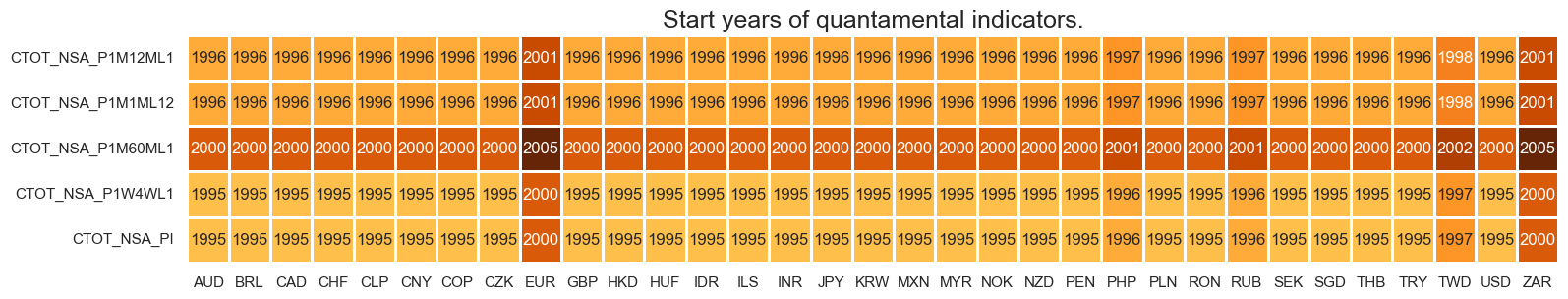
Real-time quantamental indicators of commodity-based terms-of-trade are available from 1995 for most of the countries, in line with commodity price availability. Exceptions are the Philippines and Russia (from 1996), Taiwan (1997), as well as the Eurozone and South Africa (2000).
Due to trade data availability, we use in-sample weights for the initial period when computing import and export price indices:
-
the Czech Republic, Great Britain, Hong Kong, and Norway use in-sample weights during the period 1995-01-01 / 1995-12-31
-
Poland, Romania and Thailand use in-sample weights during the period 1995-01-01 / 1996-12-31
-
Israel uses in-sample weights during the period 1995-01-01 / 1997-12-31
-
the Phillipines and Russia use in-sample weights during the period 1996-01-01 / 1998-12-31
-
Taiwan uses in-sample weights during the period 1997-01-01 / 1999-12-31
-
the Eurozone and South Africa use in-sample weights during the period 2000-01-01 / 2002-12-31
For the explanation of currency symbols, which are related to currency areas or countries for which categories are available, please view Appendix 6 .
xcatx = ctots
cidx = cids_exp

dfa = msm.reduce_df(df, xcats=xcatx, cids=cidx)
dfs = msm.check_startyears(
    dfa,
)
msm.visual_paneldates(dfs, size=(18, 3))

print("Last updated:", date.today())
Last updated: 2025-06-09
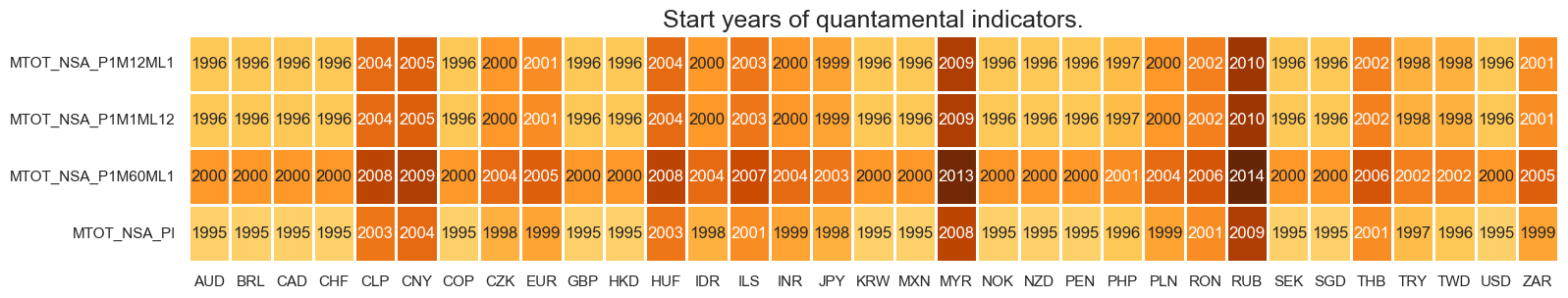
Real-time quantamental indicators of mixed terms-of-trade are mostly available from 2000, depending on the availability of the underlying data, i.e. both the commodity-based terms-of-trade and the broad import/export price indices published by each country’s statistical office.
Some countries have been publishing official terms-of-trade statistics since the 1990s or earlier:
-
Australia, Brazil, Canada, Switzerland, Colombia, Great Britain, South Korea, Mexico, Norway, New Zealand, Peru, Sweden, Singapore and the United States all have data from 1995 and are aligned with the corresponding CTOT indicator.
-
the Phillipines, the Eurozone, and South Africa have later starting dates and are also aligned with available CTOT dynamics.
-
the Czech Republic, Indonesia, India, Japan, Poland and Turkey have official import and export price series that are available from the late 1990s,
Others started later:
-
For China, Hungary, Israel, Malaysia, Romania, Russia and Thailand, official import and export price series have only been available from the 2000s.
-
Chile is a special case: due to methodology changes, price indices series are not available before 2003.
xcatx = mtots
cidx = cids_exp

dfa = msm.reduce_df(df, xcats=xcatx, cids=cidx)
dfs = msm.check_startyears(
    dfa,
)
msm.visual_paneldates(dfs, size=(18, 3))

print("Last updated:", date.today())
Last updated: 2025-06-09
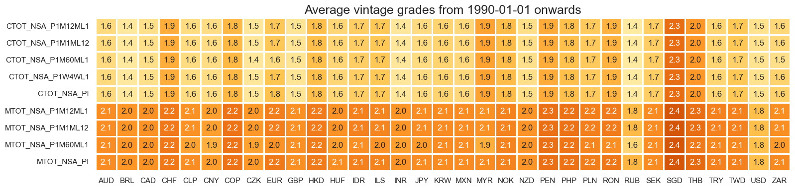
The quality of the grading is mostly a function of the trade flow data. Broad terms-of-trade information have not often been stored as vintages and is hard to procure in its original form thus far.
xcatx = ctots + mtots
cidx = cids_exp

plot = msp.heatmap_grades(
    df,
    xcats=xcatx,
    cids=cidx,
    size=(18, 4),
    title=f"Average vintage grades from {start_date} onwards",
)
History #
Terms-of-trade cumulative change #
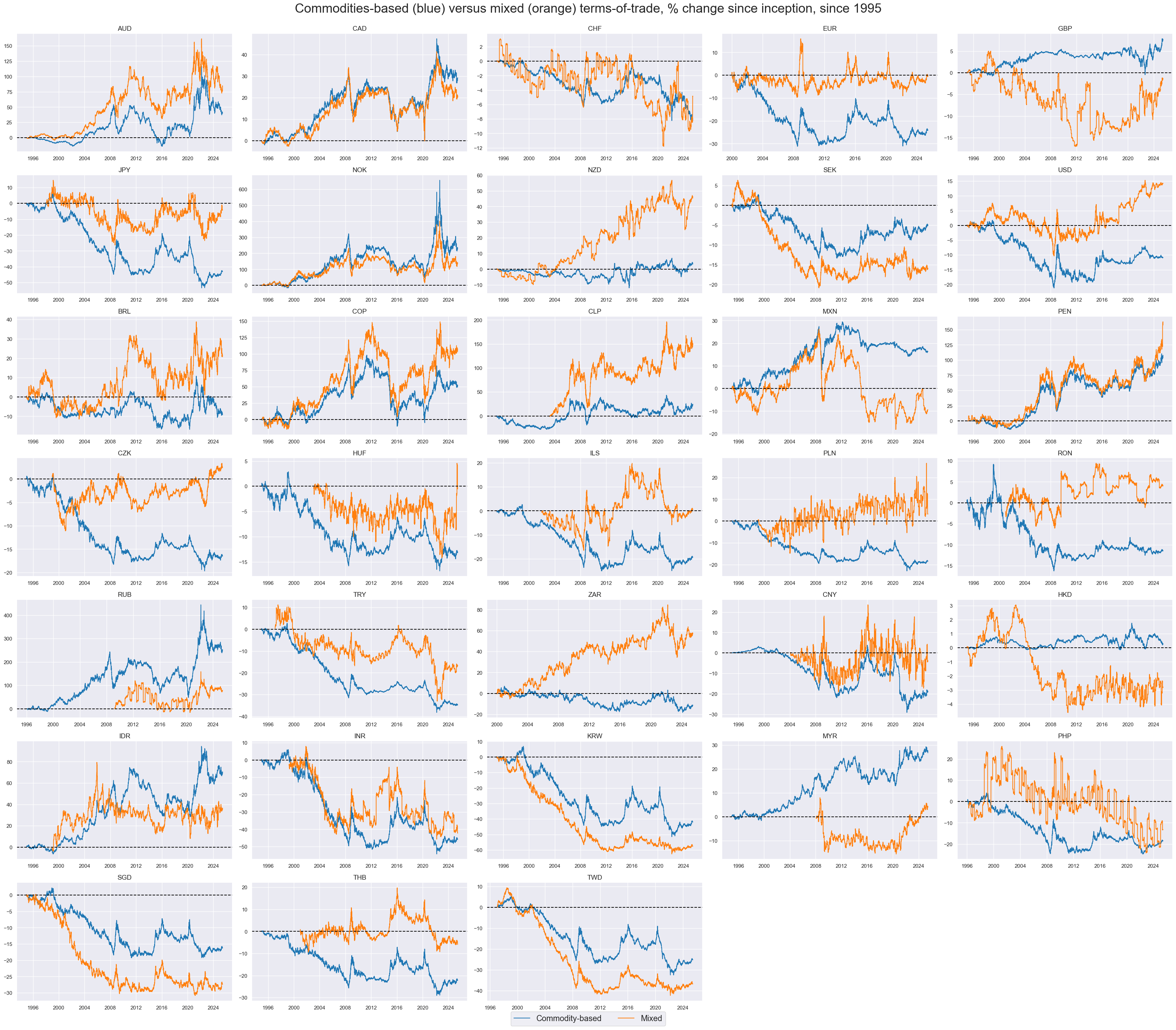
The cumulative change series conceptually measures, on each date, the % increase in the export-import ratio relative to inception. For most countries, the inception date is February 1st, 1995. For most countries, the range has been contained in a range of -40% and +80% over the past 28 years. The long-term cumulative changes have been very different across currency areas.
Note that since the index is based on a price ratio, the cumulative change series is skewed to the high side. For example, if export prices rise 3 times as much as import prices, it would reach 300%. But if import prices rise 3 times as much as export prices, it would reach 33%. For trading signals, it may be better to create a log ratio series based on this series to ensure balanced signals from positive and negative terms-of-trade changes.
There can be significant differences between commodity and mixed terms of trade, particularly for economies where commodities have little weight. Also some countries, particularly the Phillipines, show pronounced seasonality in mixed terms-of-trade, as non-commodity trade prices can be subject to greater seasonal fluctuations.
xcatx = ["CTOT_NSA_PI", "MTOT_NSA_PI"]
cidx = cids_exp

msp.view_timelines(
    df,
    xcats=xcatx,
    cids=cidx,
    start="1995-01-01",
    title="Commodities-based (blue) versus mixed (orange) terms-of-trade, % change since inception, since 1995",
    title_fontsize=27,
    legend_fontsize=17,
    xcat_labels=["Commodity-based", "Mixed"],
    ncol=5,
    same_y=False,
    size=(12, 7),
    all_xticks=True,
)
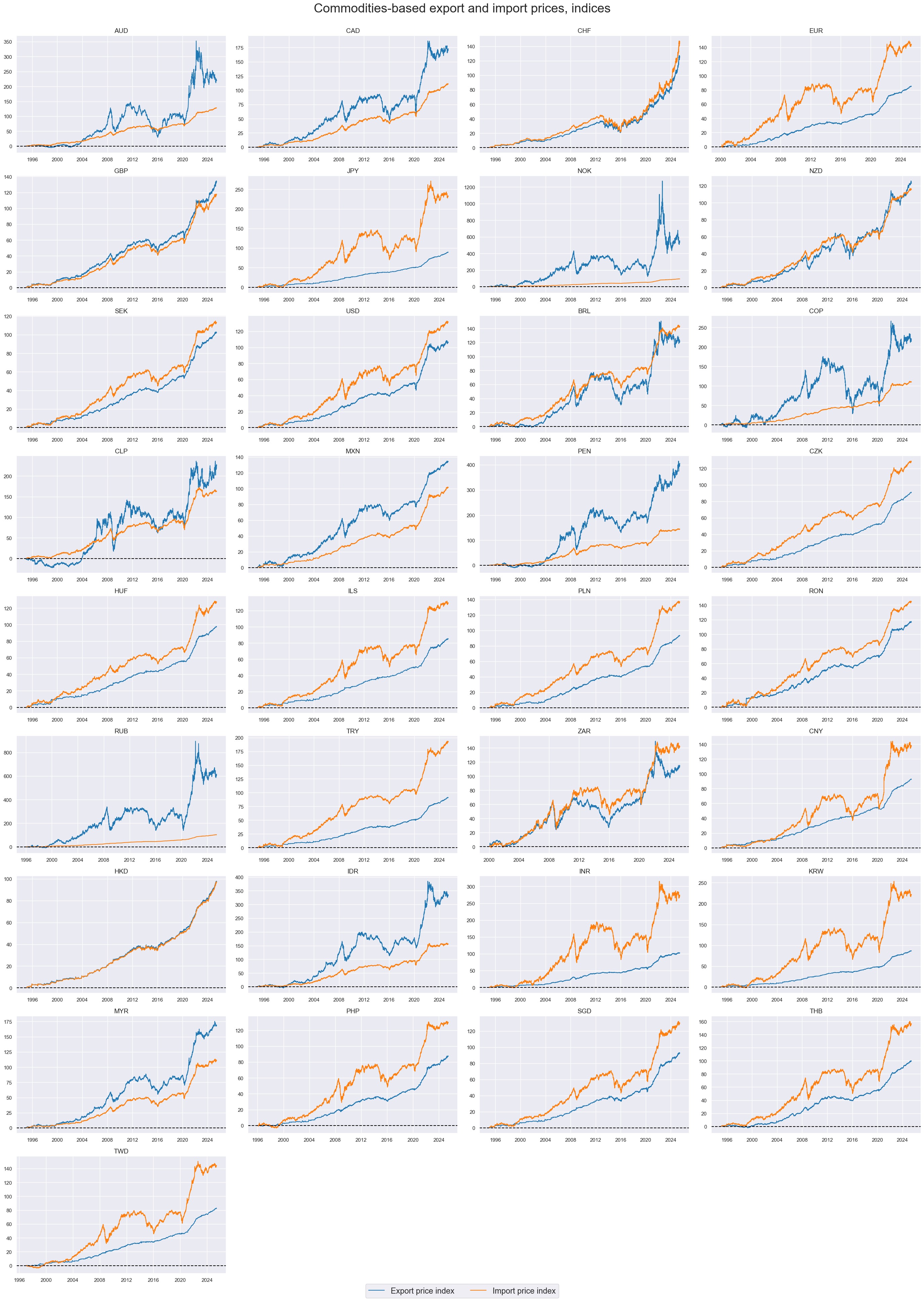
Relative commodities-based export and import price ratios change if the weight of commodities of the individual price ratios are very different and in time when commodity markets move significantly.
xcatx = ["CXPI_NSA_PI", "CMPI_NSA_PI"]
cidx = cids_exp

msp.view_timelines(
    df,
    xcats=xcatx,
    cids=cidx,
    start="1995-01-01",
    title="Commodities-based export and import prices, indices",
    xcat_labels=["Export price index", "Import price index"],
    title_fontsize=27,
    legend_fontsize=17,
    ncol=4,
    same_y=False,
    size=(12, 7),
    all_xticks=True,
)
Short-term terms-of-trade dynamics #
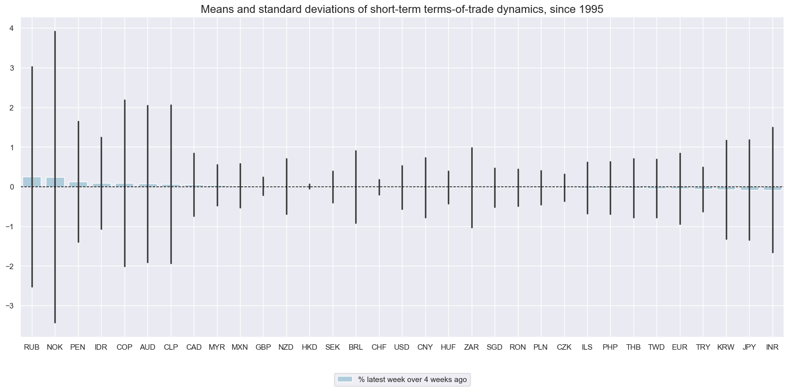
Short-term variations in terms of trade, such as latest week over previous four weeks, display very different variability, with commodity exporters and some countries with heavy reliance on commodity imports posting the greatest variation.
xcatx = ["CTOT_NSA_P1W4WL1"]
cidx = cids_exp

msp.view_ranges(
    df,
    xcats=xcatx,
    cids=cidx,
    sort_cids_by="mean",
    start="1995-01-01",
    title="Means and standard deviations of short-term terms-of-trade dynamics, since 1995",
    xcat_labels=["% latest week over 4 weeks ago"],
    kind="bar",
    size=(16, 8),
)
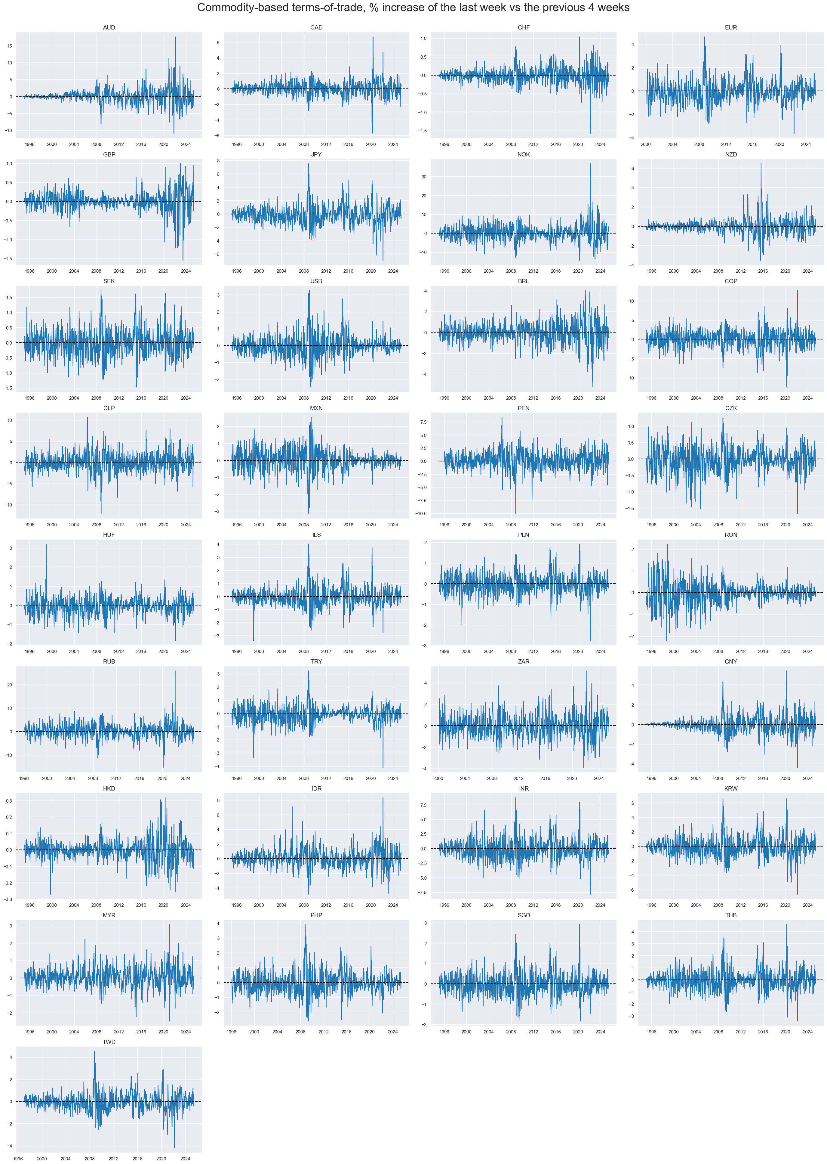
For some cross-sections, variation has been uneven across the years. This reflects mainly changes in the trade structure, such as the growing or declining importance of commodities. In some cases, the broadening of tradable commodity contracts has also affected variations.
xcatx = ["CTOT_NSA_P1W4WL1"]
cidx = cids_exp

msp.view_timelines(
    df,
    xcats=xcatx,
    cids=cidx,
    start="1995-01-01",
    title="Commodity-based terms-of-trade, % increase of the last week vs the previous 4 weeks",
    title_fontsize=27,
    ncol=4,
    same_y=False,
    size=(12, 7),
    all_xticks=True,
)
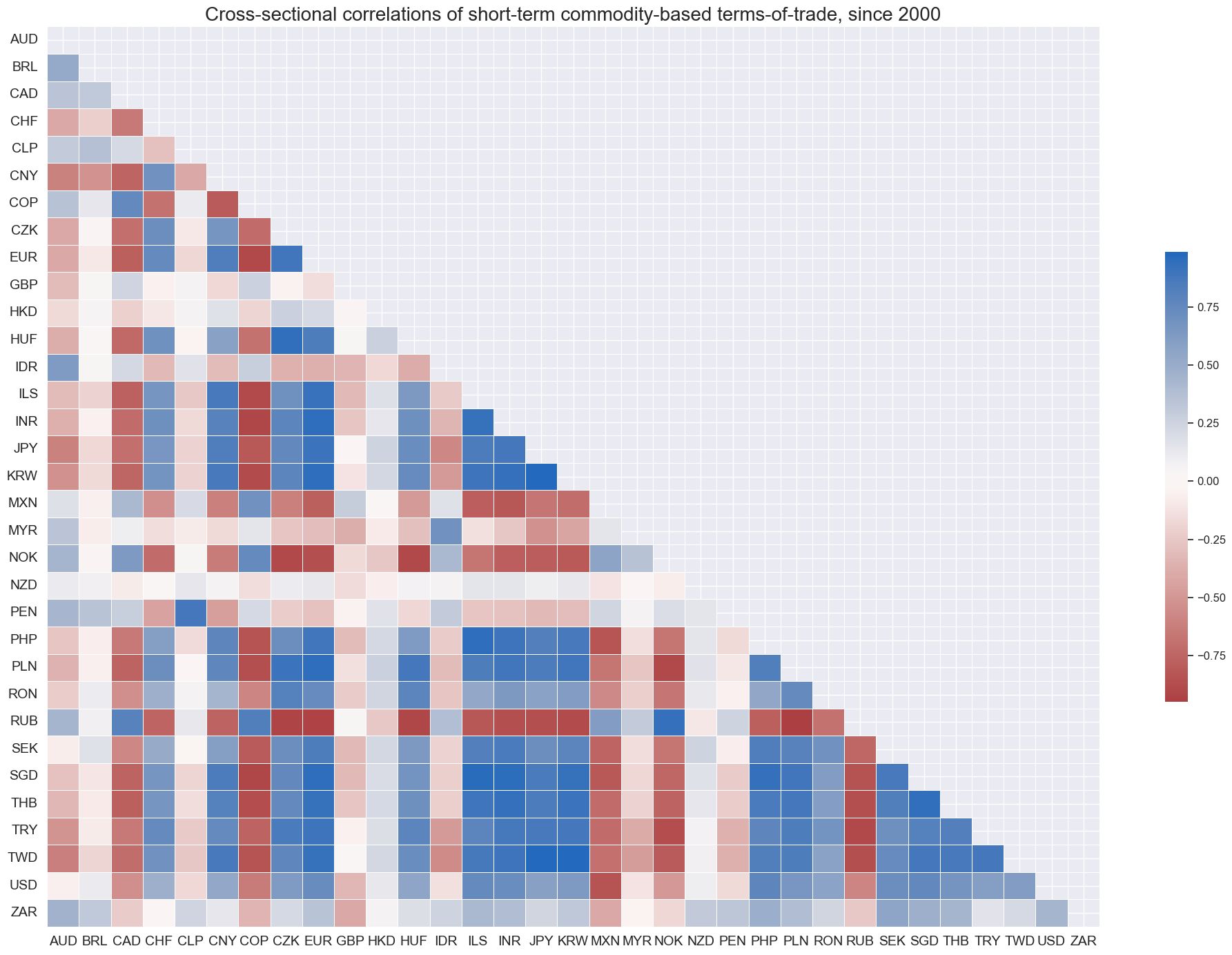
Correlation of terms of trade has been groupwise positive and negative, mostly depending on whether a currency area is a net commodity exporter or importer.
xcatx = "CTOT_NSA_P1W4WL1"
cidx = cids_exp

msp.correl_matrix(
    df,
    xcats=xcatx,
    cids=cidx,
    title="Cross-sectional correlations of short-term commodity-based terms-of-trade, since 2000",
    size=(20, 14),
)
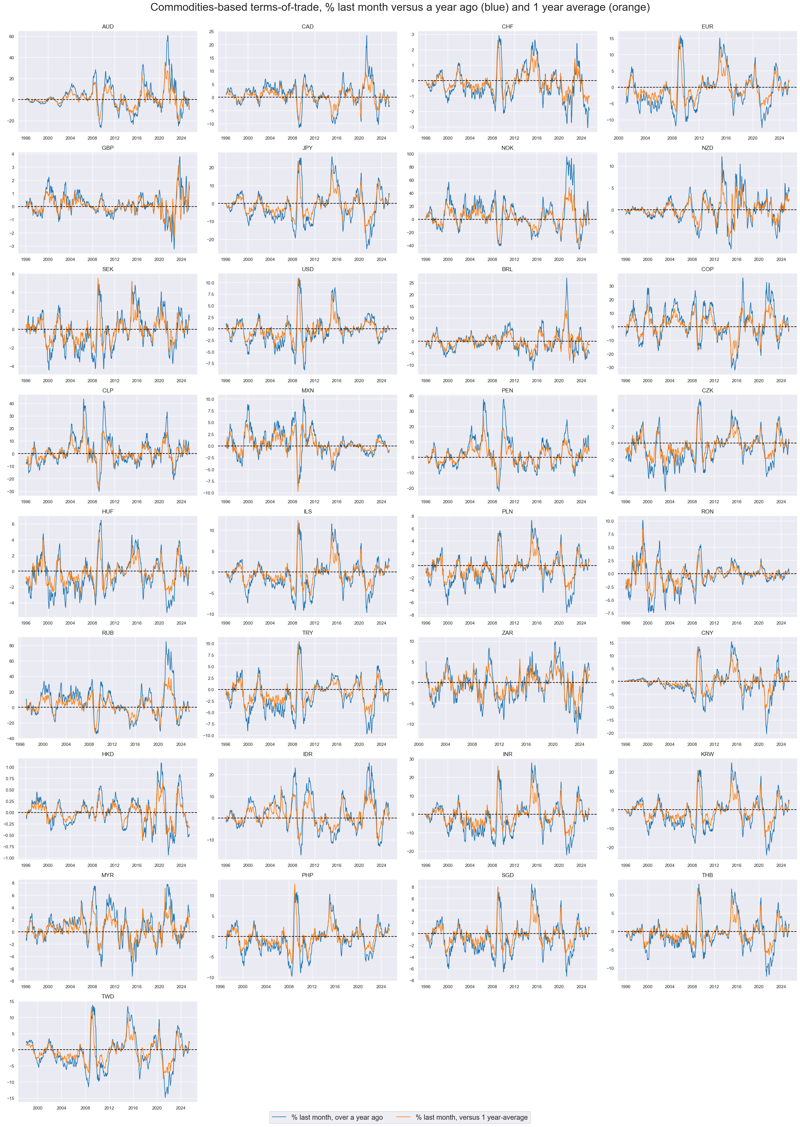
Medium-term terms-of-trade dynamics #
The medium-term terms-of-trade changes have displayed pronounced cycles in past decades, providing impetus for growth and inflation divergences across countries.
xcatx = ["CTOT_NSA_P1M1ML12", "CTOT_NSA_P1M12ML1"]
cidx = cids_exp

msp.view_timelines(
    df,
    xcats=xcatx,
    cids=cidx,
    start="1995-01-01",
    title="Commodities-based terms-of-trade, % last month versus a year ago (blue) and 1 year average (orange)",
    xcat_labels=[
        "% last month, over a year ago",
        "% last month, versus 1 year-average",
    ],
    title_fontsize=27,
    legend_fontsize=17,
    ncol=4,
    same_y=False,
    size=(12, 7),

    all_xticks=True,
)
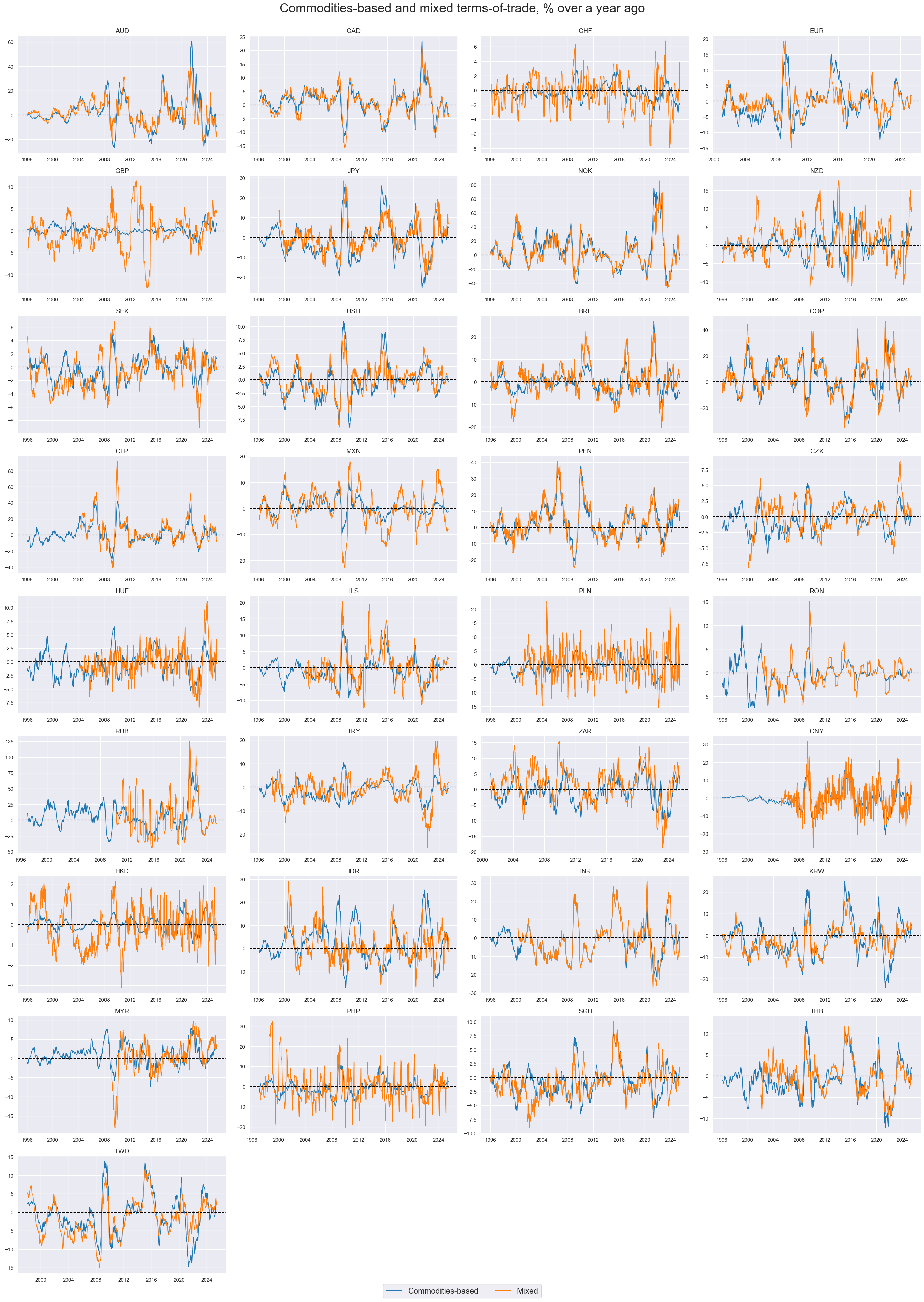
While the use of mixed terms of trade is more inclusive, it can also add volatility.
xcatx = ["CTOT_NSA_P1M1ML12", "MTOT_NSA_P1M1ML12"]
cidx = cids_exp

msp.view_timelines(
    df,
    xcats=xcatx,
    cids=cidx,
    start="1995-01-01",
    title="Commodities-based and mixed terms-of-trade, % over a year ago",
    xcat_labels=["Commodities-based", "Mixed"],
    title_fontsize=27,
    legend_fontsize=17,
    ncol=4,
    same_y=False,
    size=(12, 7),
     all_xticks=True,
)
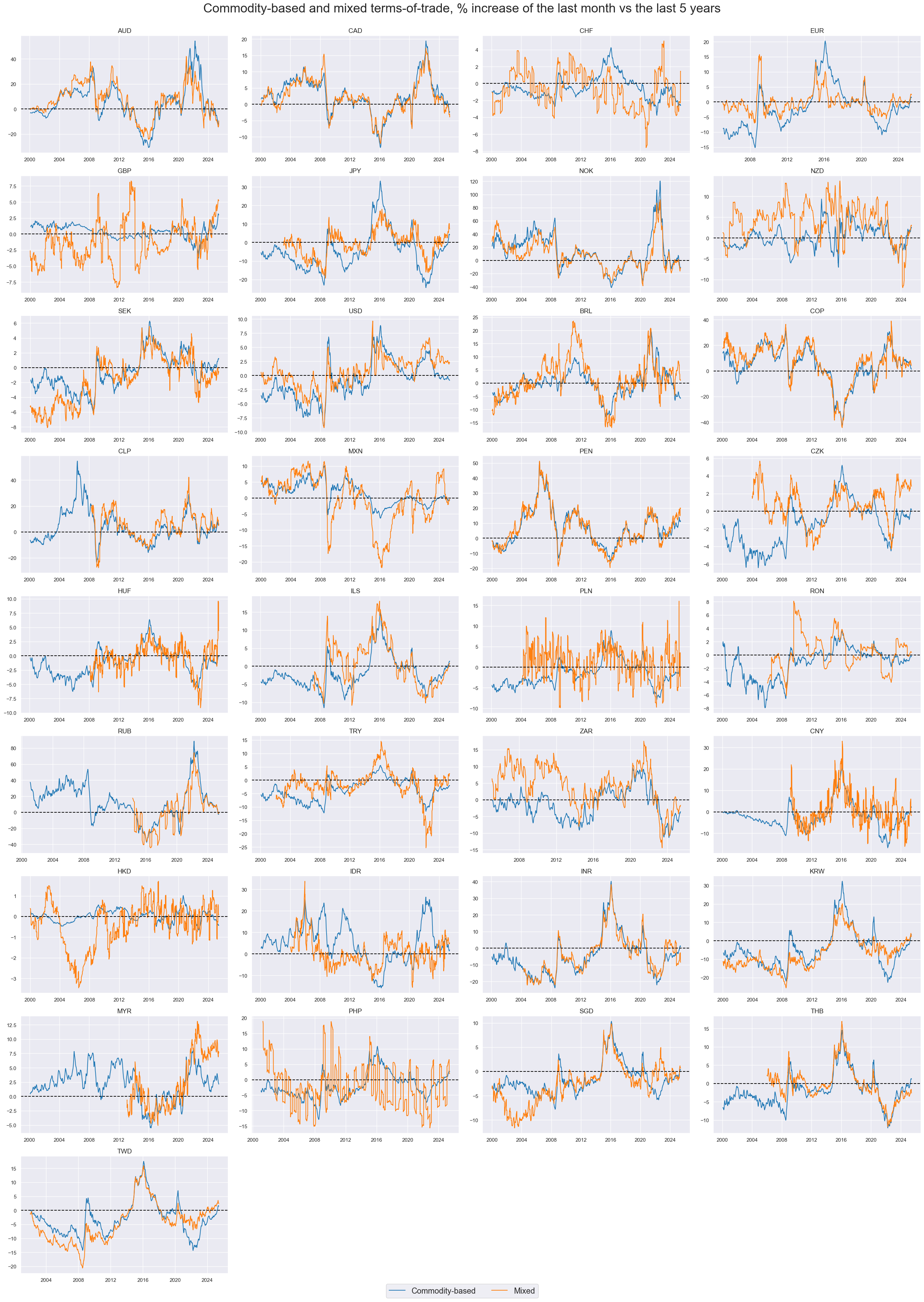
Long-term terms-of-trade dynamics #
Estimated terms-of-trade changes over 5-year averages are, by themselves, indicative of investment and medium-term economic growth conditions. However,to assess the actual impact on local economic conditions it would be best to multiply this indicator with the quantamental “openess indicator” on JPMaQS, as terms of trade usually have a greater impact on countries with a large exteranl trade share.
There is a trade-off between using commodity and mixed terms-of-trade for long-term terms-of-trade dynamics. The mixed terms of trade are naturally more inclusive and representative. The drawback is the shorter history and poor data quality in some countries, particularly those that do not publish actual price index levels. Also, seasonality adds additional volatility.
xcatx = ["CTOT_NSA_P1M60ML1", "MTOT_NSA_P1M60ML1"]
msp.view_timelines(
    df,
    xcats=xcatx,
    cids=cidx,
    start="2000-01-01",
    title="Commodity-based and mixed terms-of-trade, % increase of the last month vs the last 5 years",
    xcat_labels=["Commodity-based", "Mixed"],
    title_fontsize=27,
    legend_fontsize=17,
    ncol=4,
    same_y=False,
    size=(12, 7),

    all_xticks=True,
)
Importance #
Research links #
“We study the impact of exogenous terms-of-trade shocks in a large sample of small open economies. Using a panel vector autoregression, we estimate the response of domestic variables including the exchange rate, output, exports, imports, and domestic demand, allowing impulse responses to vary according to the de facto exchange rate regime. We find strong evidence that flexible exchange rate regimes play a shock-absorbing role by reducing the response of output to terms-of-trade shocks. Results show that flexible regimes see a stronger response of the real exchange rate and faster external adjustment, suggestive of a mechanism that switches expenditure from imported to domestically-produced goods.” Carrière-Swallow, Magud and Yépez
“In response to a fall in the terms of trade, the small and slow real depreciation observed in pegs is due to the fall in domestic prices while the large and immediate real depreciation in floats reflects a large nominal depreciation. This pattern is present in all of the time periods and regions examined… “ Broda
“Shocks that move primary commodity prices account for a large fraction of the volatility of real exchange rates…We provide empirical evidence that points toward a common factor that moves a handful of primary commodity prices on the one hand and real exchange rates between the United States and the United Kingdom, Germany, and Japan on the other. More specifically, we show that shocks that move just four primary commodity prices can account for between one-third to one-half of the volatility of the real exchange rates for a period that lasts more than half a century.” Ayres, Hevia and Nicolini
“When analyzing terms-of-trade shocks, it is implicitly assumed that the economy responds symmetrically to changes in export and import prices. Using a sample of developing countries our paper shows that this is not the case. We construct export and import price indices using commodity and manufacturing price data matched with trade shares and separately identify export price, import price, and global economic activity shocks using sign and narrative restrictions. Taken together, export and import price shocks account for around 40 percent of output fluctuations but export price shocks are, on average, twice as important as import price shocks for domestic business cycles.” Di Pace, Juvenal and Petrella
“All other things equal, an improvement in a country’s terms of trade, the ratio of export to import prices, translates into increased demand for its currency and a boost for its growth outlook. However, terms of trade are a rather subtle and sporadic influence. Therefore, many market participants are rationally inattentive to smaller changes and unwilling to trade on large changes in times of turmoil. This points to investor value in the systematic consideration of monthly or annual terms-of-trade dynamics, which can be approximated by commodity-based export and import price indices. Empirically, standard terms-of-trade dynamics have indeed predicted FX returns positively since 2000, across developed and emerging market countries. However, while this relation has been fairly stable in the developed world since 2000, for emerging markets the trading value of terms-of-trade indicators has only become evident since the great financial crisis.” Macrosynergy
Empirical clues #
Terms of trade and subsequent FX returns #
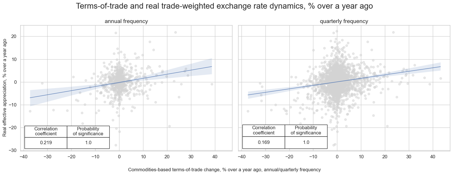
Short/medium-term terms-of-trade dynamics and subsequent hedged FX returns #
Short-term terms-of-trade changes, at all frequencies, have been positively correlated with concurrent real-effective exchange rate changes. Countries which see their export prices rising against their import prices tend to experience appreciation. From a currency trading perspective, this suggests that both changes have to be viewed together to estimate the impact of global market shocks on subsequent FX returns.
dfx = df.copy()

dfb = dfx[dfx["xcat"].isin(["FXTARGETED_NSA", "FXUNTRADABLE_NSA"])].loc[
    :, ["cid", "xcat", "real_date", "value"]
]
dfba = (
    dfb.groupby(["cid", "real_date"])
    .aggregate(value=pd.NamedAgg(column="value", aggfunc="max"))
    .reset_index()
)
dfba["xcat"] = "FXBLACK"
fxblack = msp.make_blacklist(dfba, "FXBLACK")
freqs = {"A" : "annual frequency",
         "Q": "quarterly frequency"}

relations = []

for freq in list(freqs.keys()):
    cr = msp.CategoryRelations(
        dfx,
        xcats=["CTOT_NSA_P1M12ML1", "REER_NSA_P1M12ML1"],
        cids=cids_fx,
        freq=freq,
        lag=0,
        xcat_aggs=["last", "last"],
        start="2000-01-01",
        blacklist = fxblack
    )
    relations.append(cr)

msv.multiple_reg_scatter(
        relations,
        title="Terms-of-trade and real trade-weighted exchange rate dynamics, % over a year ago",
        xlab="Commodities-based terms-of-trade change, % over a year ago, annual/quarterly frequency",
        ylab="Real effective appreciation, % over a year ago",
        ncol=2,
        nrow=1,
        figsize=(16, 6),
        prob_est="map",
        coef_box="lower left",
        subplot_titles=list(freqs.values()),
     )
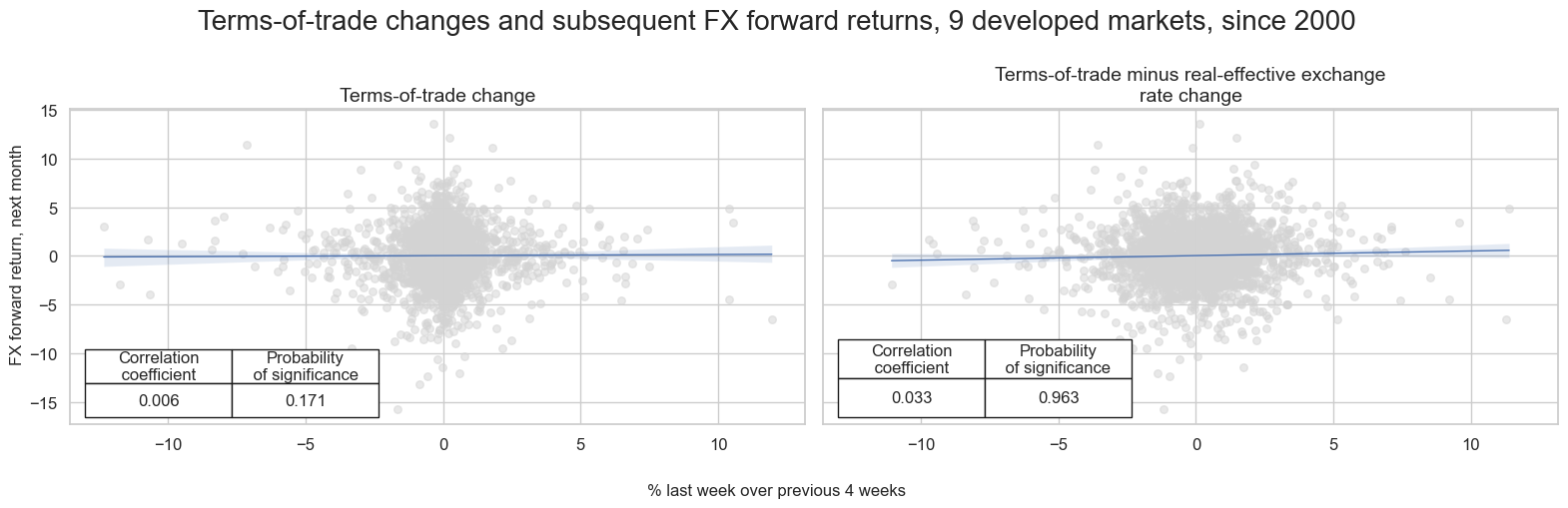
There is more direct evidence that terms-of-trade changes predict future FX returns mainly when viewed in conjunction with concurrent real-effective exchange rate changes. 1-month forward predictive power of outright (commodity-based) terms-of-trade changes (one week versus previous 4 weeks) for next month FX forward returns of developed market currencies has been insignificant. However, the predictive power of the difference between terms-of-trade changes and concurrent real-effective exchange rate changes has been been positive and significant with over 95% confidence.
cidx = cids_dmfx + ["EUR"]
tf = "_P1W4WL1"
dfa = msp.panel_calculator(
    dfx, calcs=[f"TR{tf} = CTOT_NSA{tf} - REER_NSA{tf}"], cids=cidx, start="2000-01-01"
)
dfx = msm.update_df(dfx, dfa)

xcatx = {
    f"CTOT_NSA{tf}": "Terms-of-trade change",
    f"TR{tf}": "Terms-of-trade minus real-effective exchange rate change",
}

# Create the CategoryRelations objects
relations = []
for xcat in xcatx.keys():
    cr = msp.CategoryRelations(
        dfx,
        xcats=[xcat, "FXXR_NSA"],
        cids=cidx,
        freq="m",
        lag=1,
        xcat_aggs=["last", "sum"],
        start="2000-01-01",
        blacklist=fxblack,
    )
    relations.append(cr)

subplot_titles = list(xcatx.values())

# Plot the results
msv.multiple_reg_scatter(
    relations,
    title=f"Terms-of-trade changes and subsequent FX forward returns, {len(cidx)} developed markets, since 2000",
    xlab="% last week over previous 4 weeks",
    ylab="FX forward return, next month",
    ncol=2,
    nrow=1,
    figsize=(16, 5),
    prob_est="map",
    coef_box="lower left",
    subplot_titles=subplot_titles,
)
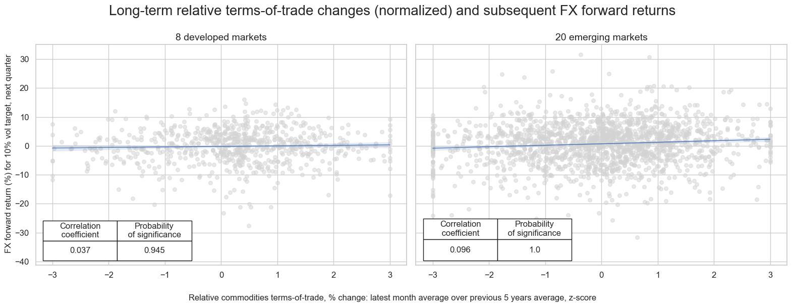
Relative long-term terms-of-trade dynamics and subsequent FX forward returns #
Relative normalized long-term commodity-based terms-of-trade trends have displayed positive predictive power for subsequent FX forward returns. Relative here means terms-of-trade changes of a reference currency versus its natural benchmark, i.e., either euro or dollar. Long-term here means the latest month over the previous 5 years. Trends have been normalized to account for differences in economic structure and trading partners across countries. Positive predictive power has been significant for both developed and emerging market currencies, with the latter being more pronounced. The predictive power has been particularly strong for commodity exporters, such as
AUD
,
NOK
,
BRL
,
ZAR
.
xcatx = ctots + imps

for xc in xcatx:
    calc_eur = [f"{xc}vBM = {xc} - iEUR_{xc}"]
    calc_usd = [f"{xc}vBM = {xc} - iUSD_{xc}"]
    calc_eud = [f"{xc}vBM = {xc} - 0.5 * ( iEUR_{xc} + iUSD_{xc} )"]

    dfa_eur = msp.panel_calculator(dfx, calcs=calc_eur, cids=cids_eur)
    dfa_usd = msp.panel_calculator(dfx, calcs=calc_usd, cids=cids_usd + ["EUR"])
    dfa_eud = msp.panel_calculator(dfx, calcs=calc_eud, cids=cids_eud)

    dfa = msm.update_df(dfa, pd.concat([dfa_eur, dfa_usd, dfa_eud]))

dfx = msm.update_df(dfx, dfa)


dfa = msp.make_zn_scores(
        dfx,
        xcat="CTOT_NSA_P1M60ML1vBM",
        cids=cids_fx,
        sequential=True,
        min_obs=261 * 5,
        neutral="zero",
        pan_weight=0,  # 50% cross-section weight as ToT changes are not fully comparable
        thresh=3,
        postfix="_ZN",
        est_freq="m",
    )

dfx = msm.update_df(dfx, dfa)
# Define region-specific configs
regions = [
    {"name": "Developed Markets", "cids": cids_dmfx},
    {"name": "Emerging Markets", "cids": cids_emfx}
]

# Store results in a dictionary
cr = {}

for region in regions:
    cr[region["name"]] = msp.CategoryRelations(
        dfx,
        xcats=['CTOT_NSA_P1M60ML1vBM_ZN', "FXXR_VT10"],
        cids=region["cids"],
        freq="q",
        lag=1,
        xcat_aggs=["last", "sum"],
        start="2000-01-01",
        blacklist=fxblack,
    )


msv.multiple_reg_scatter(
    cat_rels=[cr["Developed Markets"], cr["Emerging Markets"]],
    title="Long-term relative terms-of-trade changes (normalized) and subsequent FX forward returns",
    xlab="Relative commodities terms-of-trade, % change: latest month average over previous 5 years average, z-score",
    ylab="FX forward return (%) for 10% vol target, next quarter",
    ncol=2,
    nrow=1,
    figsize=(16, 6),
    prob_est="map",
    coef_box="lower left",
    subplot_titles=[f"{len(cids_dmfx)} developed markets", f"{len(cids_emfx)} emerging markets"]
)
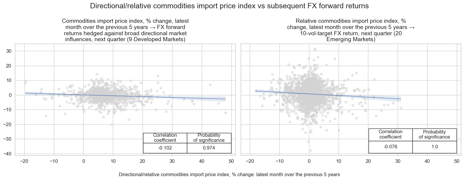
Commodity-based import price dynamics vs subsequent FX forward returns #
Commodity-based import prices hold negative predictive power for subsequent FX returns. In developed markets, this effect is strongest for FX forward returns hedged against broad market direction risk (
FXXRHvGDRB_NSA
).
In emerging markets, the impact is most evident in unhedged FX forward returns targeting a 10% volatility level using the dominant cross (
FXXR_VT10
).
# Define signal-target-region configurations
analysis_configs = [
    {
        "sig": "CMPI_NSA_P1M60ML1",
        "sig_label": "Commodities import price index, % change, latest month over the previous 5 years",
        "targ": "FXXRHvGDRB_NSA",
        "targ_label": "FX forward returns hedged against broad directional market influences, next quarter",
        "cids": cids_dmfx + ["EUR"],
        "region": "Developed Markets"
    },
    {
        "sig": "CMPI_NSA_P1M60ML1vBM",
        "sig_label": "Relative commodities import price index, % change, latest month over the previous 5 years",
        "targ": "FXXR_VT10",
        "targ_label": "10-vol-target FX return, next quarter",
        "cids": cids_emfx,
        "region": "Emerging Markets"
    }
]

# Generate regression objects and titles
rel_list = []
subplot_titles = []

for cfg in analysis_configs:
    rel = msp.CategoryRelations(
        dfx,
        xcats=[cfg["sig"], cfg["targ"]],
        cids=cfg["cids"],
        freq="Q",
        lag=1,
        xcat_aggs=["last", "sum"],
        blacklist=fxblack,
        start="2000-01-01",
        xcat_trims=[60, 60],
    )
    rel_list.append(rel)
    subplot_titles.append(f"{cfg['sig_label']} → {cfg['targ_label']} ({len(cfg['cids'])} {cfg['region']})")

msv.multiple_reg_scatter(
    cat_rels=rel_list,
    ncol=2,
    nrow=1,
    figsize=(16, 6),
    title="Directional/relative commodities import price index vs subsequent FX forward returns",
    title_fontsize=18,
    xlab="Directional/relative commodities import price index, % change: latest month over the previous 5 years",
    ylab="",
    coef_box="lower right",
    prob_est="map",
    subplot_titles=subplot_titles,
)
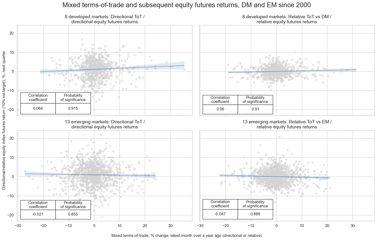
Terms of trade improvement and equity futures returns #
Improvements in terms of trade exhibit some positive predictive power for both directional and relative future equity returns in developed markets. Such improvements can enhance national income and corporate profitability. In contrast, the relationship reverses in emerging markets, although the negative correlation falls short of statistical significance.
xcatx = ["EQXR_NSA", "EQXR_VT10"] + main

region_map = {
    "vDM": cids_dmeq,
    "vEM": cids_emeq,
}

for postfix, cids in region_map.items():
    dfa = msp.make_relative_value(
        dfx,
        xcats=xcatx,
        cids=cids,
        start="2000-01-01",
        rel_meth="subtract",
        complete_cross=False,
        postfix=postfix,
    )
    dfx = msm.update_df(dfx, dfa)
region_configs = {
    "DM": {
        "signal_pairs": [
            ("MTOT_NSA_P1M1ML12", "EQXR_VT10"),
            ("MTOT_NSA_P1M1ML12vDM", "EQXR_VT10vDM")
        ],
        "cids": cids_dmeq,
        "subplot_titles": [
            f"{len(cids_dmeq)} developed markets: Directional ToT / directional equity futures returns",
            f"{len(cids_dmeq)} developed markets: Relative ToT vs DM / relative equity futures returns"
        ],
    },
    "EM": {
        "signal_pairs": [
            ("MTOT_NSA_P1M1ML12", "EQXR_VT10"),
            ("MTOT_NSA_P1M1ML12vEM", "EQXR_VT10vEM")
        ],
        "cids": cids_emeq,
        "subplot_titles": [
            f"{len(cids_emeq)} emerging markets: Directional ToT / directional equity futures returns",
            f"{len(cids_emeq)} emerging markets: Relative ToT vs EM / relative equity futures returns"
        ],
    }
}

# Collect all CategoryRelations objects and subplot titles
all_relations = []
all_titles = []

for region, config in region_configs.items():
    for i, (sig, targ) in enumerate(config["signal_pairs"]):
        cr = msp.CategoryRelations(
            dfx,
            xcats=[sig, targ],
            cids=config["cids"],
            freq="Q",
            lag=1,
            xcat_aggs=["last", "sum"],
            start="2000-01-01",
        )
        all_relations.append(cr)
        all_titles.append(config["subplot_titles"][i])

# Plot all combinations
msv.multiple_reg_scatter(
    cat_rels=all_relations,
    title="Mixed terms-of-trade and subsequent equity futures returns, DM and EM since 2000",
    xlab="Mixed terms-of-trade, % change: latest month over a year ago (directional or relative)",
    ylab="Directional/relative equity index futures return (10% vol target), %, next quarter",
    ncol=2,
    nrow=2,
    figsize=(16, 10),
    prob_est="map",
    coef_box="lower left",
    subplot_titles=all_titles
)
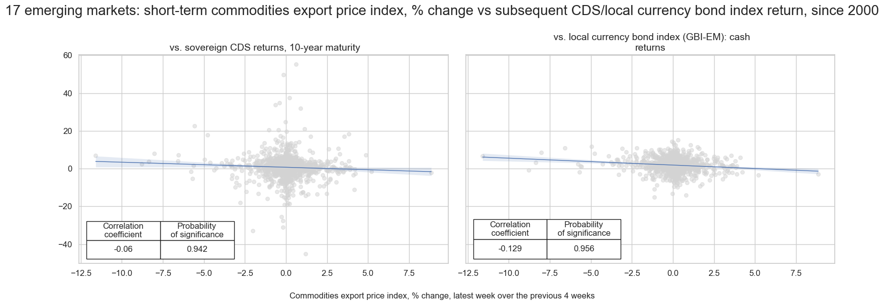
Terms-of-trade and sovereign CDS/ local currency bond index returns in emerging markets #
In emerging markets, rising terms-of-trade, often driven by stronger commodity exports, signal improved external balances and lower sovereign risk. This typically leads to tighter CDS spreads, implying negative predictive power of terms-of-trade changes for subsequent CDS returns.
sigx = {
    "CXPI_NSA_P1W4WL1": "Commodities export price index, % change, latest week over the previous 4 weeks",
      }

targx = {
    "CDS10YXR_NSA": "sovereign CDS returns, 10-year maturity",
    "LCBIR_NSA": "local currency bond index (GBI-EM): cash returns",
      }

# Define cross-section (market) groups
cidx = msm.common_cids(dfx, xcats=list(sigx.keys()) + list(targx.keys()))
cidx = list(set(cidx) & set(cids_em))

# Dictionary to store CategoryRelations objects
cr = {}

# Iterate through markets and matched signals/targets

for targ in targx.keys():
        cr[f"cr_{targ}"] = msp.CategoryRelations(
                dfx,
                xcats=[list(sigx.keys())[0], targ],
                cids=list(cidx),
                freq="q",
                lag=1,
                xcat_aggs=["last", "sum"],
                blacklist=fxblack,
                start="2000-01-01",
                xcat_trims=[60, 60],  # Trimming to remove outliers
            )

# Store all CategoryRelations instances in a list
all_cr_instances = list(cr.values())

subplot_titles = [
    f" vs. {targx[targ]}"
    for targ in targx.keys()
]


msv.multiple_reg_scatter(
        all_cr_instances,
        title=f"{len(cidx)} emerging markets: short-term commodities export price index, % change vs subsequent CDS/local currency bond index return, since 2000" ,
        xlab=list(sigx.values())[0],
        ylab="",
        ncol=2,
        nrow=1,
        figsize=(16, 6),
        prob_est="map",
        subplot_titles = subplot_titles,
        coef_box="lower left",
)
Appendices #
Appendix 1: How commodity-based price indices are computed #
Terms-of-trade is the ratio of a country’s export price index to its import price index. Conceptually, it measures the quantity of an abstract good a country can import for a unit of abstract good that it exports.
Conventionally, it is the weighted average of export prices (export price index, XPI) divided by the weighted average of import prices (import price index, MPI). All prices shall be quoted in USD. However, the ratio is a unit-less quantity and it is tracked as an index.
Both numerator and denominator of a terms-of-trade index in JPMaQS are calculated are calculated in the form of Laspeyres indices. This means that the export and import quantities of the index are fixed to a base period. The importance of a traded good’s price in the export or import price index depends on its traded quantity in a base period and the price itself. The generic for the export price index, for example, looks as follows
where \(Q[x]_{t, i}\) denote the \(i^{th}\) good’s export quantity in physical units in period t, and \(P[x]_{t, i}\) I refers to the unit price of export good \(i\) in period t.
Period \(t=0\) here refers to a base period for the calculation of the index.
Alternatively, we can express the export price index is as a weighted sum of price ratios: $ \( XPI_t= \sum_{i} \frac{P[x]_{t,i}}{P[x]_{0,i}} \cdot \omega[x]_{0, i} \) $
where the weight of each good is its share in total export value in the base period:
where the denominator is the sum over the export values of all goods (indexed by j).
These weights can be derived from annual trade value statistics.
The implementation of approximate commodity terms-of-trade in JPMaQS required three practical modifications of these general formulas.
-
First, only a subset of exports and imports can be associated to daily proxy prices, these typically being commodity goods with global or regional tracked contracts. This means we need to distinguish between commodities (c) and non-commodities (nc). The set of goods with available daily price is referred to as “commodities”, of size \(N_c\) and indexed with \(j\) . The remaining set of goods is referred to as “non-commodities”, of size \(N_{nc}\) and indexed with \(k\) . They clearly sum up to \(N = N_c + N_{nc}\) different goods.
with the export trade share for a general good \(i\)
Typically, we have no information on non-commodity prices or even some commodities that are not quoted in markets. This means that the price index equation simplifies:
where \(P_{t}\) is a generic tradable goods price index that represents international non-commodity goods price inflation. JPMaQS uses the U.S. core PPI for this purpose.
-
Representative export and import weights change overtime and, hence, weights need to be updated. We do so by first calculating monthly price indices and then chaining them. We use a double time index \((m, d)\) instead of \(t\) , where the first element represent the month and the second is the specific trading day. \(ld\) is the last trading day available in that month.
The monthly price indices are calculated in the following way, so that it has a base period value of 1 at the beginning of each period \(m\) .
where \(\omega[x_c]_{m,j}\) refers to the weight of good j estimated for month \(m\) based on the information set at the end of month \(m-1\) .
To concatenate the monthly price indices, we simply need to multiply the latest month’s index values with the product of all previous months’ endpoints:
-
Global core producer prices are not available on daily basis and they may not even be available for the concurrent month at all. Hence the daily produce price needs to be interpolated and potentially estimated.
When the PPI data has been published for a given month \(m\) , then we can interpolate this price growth over the month. $ \( \frac{P_{m, d}}{P_{m, 0}} = (1+\pi_{m})^{d / D_m} \) $
For the most recent months in each vintage, it is possible that the PPI data has not been published yet so we need to estimate this quantity daily: $ \( \frac{P_{m, d}}{P_{m, 0}} = (1+ Est[\pi_{m}])^{d / D_m} \) $
where \(D_m\) is the number of trading days in month \(m\) .
Appendix 2: Combining broad and commodity-based terms of trade to mixed terms of trade #
Mixed terms of trade combine broad terms of trade data, conceptually encompassing all foreign trade items, and commodity-based terms of trade data.
Broad external trade flows and corresponding price indices are being published by most countries, albeit with significant lags and typically at monthly or quarterly frequency. Compared with daily real-time commodity-based data they often look out-of-date and are therefore neglected by market participants. The mixed terms of trade concept is based on export and import price indices that use broad terms of trade for medium-term changes and commodities-based terms of trade for daily interpolation and prediction to the latest day.
Technically speaking we calculate first mixed export and import price indices, based on these two types of constituent price indices ( BXPI and BMPI ):
-
The first type uses official export and import price indices as released by national statistics offices of similar agencies, which we call broad price indices ( BXPI and BMPI ). They are based on the prices of all foreign trade items. These typically have monthly or quarterly frequency and can have a few months lag between release and the observation period.
-
The second type are the JPMaQS commodity terms of trade (**CXPI**, **CMPI**) using primary commodity trade and related market prices only. These are available daily at the beginning of the next trading day.
In the first stage of calculation, the two types of price indices are computed separately in form of vintages for equal history with an index starting point of 1 for the first day. Naturally index valuse are strictly positive. The second stage the two types are combined such that the broad lower-frequency index, anchors the long-term average of the vintages and the commodity price index is used for interpolation and predictions.
For the case of export price and monthly broad terms of trade the combined value is:
where t is a trading day and m the average of the concurrent or latest available month. Lower frequency values are considered averages because the use of period averages is a common method for measuring these price indices (at least conceptually). If t is a day of month m this formula implies interpolation. If t is a day after (the latest available) month m the formula implies prediction.
A few countries (China, Hungary, Poland, Russia) do not release their broad import/export prices as index. They only inform about a percentage change over a year ago. We refer to this format as BXPIPCT and BMPIPCT . This means that index levels must be estimated based on these changes and available levels of the commodity export or import index.
The first step is to use the commodity price index, as low-frequency averages, to estimate the broad price index levels in the first year. For the export price index and assuming a monthly broad index frequency this applies the following formula:
The second step is to use the offically provided broad index change to calculate all subsequent broad index levels:
Appendix 3: Commodity data inputs #
The commodity export and import values for all countries are taken from the United Nations Comtrade database. The frequency of the data has been monthly since 2010. Prior to 2010 the frequency was annual. Trade shares of individual commodities are export/import values divided by the corresponding period’s aggregate import and export values, which come from a variety of sources. Therefore, since 2010 trade shares have been updated monthly with the appropriate publication lag. Taiwan only provides annual releases of commodity export and import values and, hence, trade shares are updated less frequently.
Shares are computed based on a rolling window of three years of trade values, based on the concurrent vintage.
We use a comprehensive set of commodities and corresponding commodity prices to approximate as best as we can the daily move of the true (unobserved) terms-of-trade. Commodity-based and mixed terms-of-trade indicators use 35 commodities at the start in 1995, growing up to 44 in 2005 and reaching 55 from 2010 afterwards.
We can break them down into sub-categories, explicitly mentioning the first year they are available:
-
Energy:
-
Coal:
-
NYMEX Coal (pre 2006)
-
ICE Coal Richard Bay (2006)
-
ICE Coal Rotterdam (2006)
-
ICE Newcastle Coal (2006)
-
-
Crude oil:
-
Brent Forties Oseberg FOB (1970)
-
NYMEX WTI light crude (1983)
-
-
Ethanol: CBOT Ethanol (2006)
-
Gasoline: NYMEX RBOB Gasoline (2005)
-
Liquefied natural gas: Liquid Natural Gas FOB Asia (2010)
-
Natural gas:
-
NYMEX natural gas Henry Hub (1995)
-
TTF base load (2010)
-
-
Propane: Propane Spot FOB Mont Belvieu (1992)
-
-
Industrial Metals:
-
Aluminium: London Metal Exchange aluminium (1995)
-
Cobalt: London Metal Exchange cobalt (2010)
-
Copper: COMEX copper (1989)
-
Lead: London Metal Exchange Lead (1995)
-
Iron ore:
-
HWWI Iron Ore & Steel Scrap index (weekly, 2001-2007)
-
Steel Home Iron Ore FE63.5% CIF (2007)
-
-
Molybdenum: Molybdenum MO3 CIF (1993)
-
Nickel: London Metal Exchange Nickel (1995)
-
Rhodium: Rhodium spot for North West Europe CIF (1993)
-
Tin: London Metal Exchange Tin (1995)
-
Zinc: London Metal Exchange Zinc (1995)
-
-
Precious metals
-
Gold: COMEX gold 100 Ounce (1992)
-
Palladium: NYMEX palladium (1995)
-
Platinum: NYMEX platinum (1995)
-
Silver: COMEX silver 5000 Ounce (1992)
-
-
Softs:
-
Cocoa:
-
CSCE Cocoa (1979)
-
LIFFE Cocoa (1979)
-
-
Coffee: NYBOT / ICE coffee ‘C’ Arabica (1995)
-
Cotton: NYBOT / ICE cotton #2 (1995)
-
Dry whey: CME dry whey (2007)
-
Lumber: Chicago Mercantile Exchange random length lumber (1995)
-
Milk: Chicago Mercantile Exchange milk class IV (2000)
-
Milk powder (skimmed):
-
EU Agricultural Market Skimmed Milk Powder (weekly, 2001-2010)
-
Global Dairy Trade Milk powder skim (2010)
-
-
Milk powder (whole):
-
EU Agricultural Market Whole Milk Powder (weekly, 2001-2008)
-
Global Dairy Trade Milk powder whole (2008)
-
-
Orange juice concentrate: NYBOT / NYCE FCOJ frozen orange juice concentrate (1995)
-
Refined sugar: LIFFE White sugar (1989)
-
Sugar:
-
NYBOT / ICE raw cane sugar #11 (1995)
-
NYBOT / ICE raw cane sugar #16 (2008)
-
-
Tea: Tea Best Pekoe Fannings 1 Kenya (1993)
-
-
Grains:
-
Barley: Barley Minneapolis (1995)
-
Corn:
-
Chicago Board of Trade corn composite (1995)
-
MATIF Corn (2002)
-
-
Oats: Chicago Board of Trade oats (2006)
-
Soy beans: Chicago Board of Trade soybeans composite (1995)
-
Soymeal: Chicago Board of Trade soybean meal (2006)
-
Soybean oil: Chicago Board of Trade soybean oil (1975)
-
Rapeseed oil: Rapeseed Oil Dutch FOB North West Europe
-
Palm oil: Malaysian Palm Oil Crude CIF Rotterdam (1995)
-
Rice: White Rice 100pct FOB Bangkok (2008)
-
-
Wheat:
-
Chicago Board of Trade wheat composite (1995)
-
LIFFE Wheat (1989)
-
MATIF Wheat (1998)
-
-
Livestock:
-
Live cattle: Chicago Mercantile Exchange (1995)
-
Cattle feeder: Chicago Mercantile Exchange Feeder Cattle Composite (1978)
-
Hogs: Chicago Mercantile Exchange Lean Hogs Composite (1995)
-
Salmon: Fish pool salmon (2008)
-
Fish meal: Fish meal 65% Peru CIF Germany (1999)
-
-
Chemicals:
-
Urea:
-
Urea FOB Arab Gulf (2009)
-
Urea FOB US Gulf (2009)
-
Urea ammonium nitrate (UAN):
-
Urea Ammonium Nitrate 30% FOT France (2008)
-
Urea Ammonium Nitrate 30% FOT New Orleans (2008)
-
Diammonium Phosphate (DAP): Diammonium Phosphate CF New Orleans (2002)
-
Rubber: RSS3 smoked rubber sheets (1992)
-
-
Most of the commodity prices approximate well the trade activity happening over different geographies, so we associate the cross-section identifiers to these commodity prices.
In certain regions, we identify better price proxies for specific commodities, which allows us to improve the terms-of-trade estimation on a daily basis: coal, crude oil, natural gas, cocoa, sugar, corn, wheat, urea, and urea ammonium nitrate.
Show code cell content
comm_cid_map = {
    "Coal": {
        "default": "ICE Richard Bay",
        "Asia": "ICE Newcastle",
        "Europe": "ICE Rotterdam",
    },
    "Crude oil": {
        "default": "ICE Brent",
        "North America": "NYMEX WTI",
    },
    "Ethanol": {"default": "CBOT"},
    "Gasoline": {"default": "NYMEX"},
    "Propane": {"default": "Spot FOB Mont Belvieu"},
    "LNG": {"default": "Liquid Natural Gas FOB Asia"},
    "Natural gas": {"default": "NYMEX Henry Hub", "Europe": "TTF base load"},
    "Cocoa": {"default": "CSCE", "Europe": "LIFFE"},
    "Coffee": {"default": "NYBOT ICE"},
    "Orange juice": {"default": "NYBOT NYCE"},
    "Tea": {"default": "Best Pekoe Fannings"},
    "Milk": {"default": "CME"},
    "Milk powder s.": {"default": "Global dairy trade"},
    "Milk powder w.": {"default": "Global dairy trade"},
    "Dry whey": {"default": "CME"},
    "Sugar": {
        "default": "NYBOT ICE n11",
        "North America": "NYBOT ICE n16",
    },
    "White sugar": {"default": "SGW"},
    "Barley": {"default": "BAR"},
    "Corn": {"default": "CBOT", "Europe": "MATIF"},
    "Oats": {"default": "CBOT"},
    "Palm oil": {"default": "CBOT"},
    "Rapseed oil": {"default": "Dutch FOB North west Europe"},
    "Rice": {"default": "White Rice 100pct FOB Bangkok"},
    "Soybean meal": {"default": "CBOT"},
    "Soybean oil": {"default": "CBOT"},
    "Soybeans": {"default": "CBOT"},
    "Wheat": {
        "default": "CBOT",
        "UK": "LIFFE",
        "Europe": "MATIF (ex-GBP)",
    },
    "Cotton": {"default": "NYBOT ICE"},
    "Lumber": {"default": "CME"},
    "Urea": {"default": "FOB US Gulf", "Asia": "FOB Arab Gulf"},
    "UAN": {"default": "32% FOB New Orleans", "Europe": "30% FOT France"},
    "DAP": {"default": "CF New Orleans"},
    "Rubber": {"default": "RSS3 smoked sheets"},
    "Salmon": {"default": "Fishpool"},
    "Fishmeal": {"default": "65% Peru CIF Germany"},
    "Cattle": {"default": "CME"},
    "Feeder": {"default": "CME"},
    "Hogs": {"default": "CME"},
    "Aluminium": {"default": "LME"},
    "Cobalt": {"default": "LME"},
    "Copper": {"default": "COMEX"},
    "Iron ore": {"default": "Steel home"},
    "Lead": {"default": "LME"},
    "Molybdenum": {"default": "MO3 CIF"},
    "Nickel": {"default": "LME"},
    "Rhodium": {"default": "spot NWE CIF"},
    "Tin": {"default": "LME"},
    "Zinc": {"default": "LME"},
    "Gold": {"default": "COMEX"},
    "Platinum": {"default": "NYMEX"},
    "Silver": {"default": "NYMEX"},
    "Palladium": {"default": "PAL"},
}
commodity_geo_map = pd.DataFrame(comm_cid_map).fillna(value="").T
display(commodity_geo_map)
| default | Asia | Europe | North America | UK | |
|---|---|---|---|---|---|
| Coal | ICE Richard Bay | ICE Newcastle | ICE Rotterdam | ||
| Crude oil | ICE Brent | NYMEX WTI | |||
| Ethanol | CBOT | ||||
| Gasoline | NYMEX | ||||
| Propane | Spot FOB Mont Belvieu | ||||
| LNG | Liquid Natural Gas FOB Asia | ||||
| Natural gas | NYMEX Henry Hub | TTF base load | |||
| Cocoa | CSCE | LIFFE | |||
| Coffee | NYBOT ICE | ||||
| Orange juice | NYBOT NYCE | ||||
| Tea | Best Pekoe Fannings | ||||
| Milk | CME | ||||
| Milk powder s. | Global dairy trade | ||||
| Milk powder w. | Global dairy trade | ||||
| Dry whey | CME | ||||
| Sugar | NYBOT ICE n11 | NYBOT ICE n16 | |||
| White sugar | SGW | ||||
| Barley | BAR | ||||
| Corn | CBOT | MATIF | |||
| Oats | CBOT | ||||
| Palm oil | CBOT | ||||
| Rapseed oil | Dutch FOB North west Europe | ||||
| Rice | White Rice 100pct FOB Bangkok | ||||
| Soybean meal | CBOT | ||||
| Soybean oil | CBOT | ||||
| Soybeans | CBOT | ||||
| Wheat | CBOT | MATIF (ex-GBP) | LIFFE | ||
| Cotton | NYBOT ICE | ||||
| Lumber | CME | ||||
| Urea | FOB US Gulf | FOB Arab Gulf | |||
| UAN | 32% FOB New Orleans | 30% FOT France | |||
| DAP | CF New Orleans | ||||
| Rubber | RSS3 smoked sheets | ||||
| Salmon | Fishpool | ||||
| Fishmeal | 65% Peru CIF Germany | ||||
| Cattle | CME | ||||
| Feeder | CME | ||||
| Hogs | CME | ||||
| Aluminium | LME | ||||
| Cobalt | LME | ||||
| Copper | COMEX | ||||
| Iron ore | Steel home | ||||
| Lead | LME | ||||
| Molybdenum | MO3 CIF | ||||
| Nickel | LME | ||||
| Rhodium | spot NWE CIF | ||||
| Tin | LME | ||||
| Zinc | LME | ||||
| Gold | COMEX | ||||
| Platinum | NYMEX | ||||
| Silver | NYMEX | ||||
| Palladium | PAL |
Appendix 4: Broad terms-of-trade inputs #
Official import / export price indices are sourced from national sources. Depending on how each country reports them, they belong to different statistical bulletins, and have either monthly or quarterly frequency. Romania is the only region releaseing the datapoint annually.
Show code cell content
broad_df = pd.DataFrame(
    [
        {
            "Country": "Australia",
            "Source": "National statistical office",
            "Statistics group": "Balance of Payments",
            "Frequency": "Q",
            "Trade items": "Goods & Services",
        },
        {
            "Country": "Brazil",
            "Source": "FUNCEX",
            "Statistics group": "Import/Export Prices",
            "Frequency": "M",
            "Trade items": "Goods & Services",
        },
        {
            "Country": "Canada",
            "Source": "National statistical office",
            "Statistics group": "National accounts",
            "Frequency": "Q",
            "Trade items": "Goods & Services",
        },
        {
            "Country": "Chile",
            "Source": "Central bank",
            "Statistics group": "Import/Export Prices",
            "Frequency": "Q",
            "Trade items": "Goods & Services",
        },
        {
            "Country": "China",
            "Source": "General Administration of Customs",
            "Statistics group": "Import/Export Prices",
            "Frequency": "M",
            "Trade items": "Goods & Services",
        },
        {
            "Country": "Colombia",
            "Source": "Central bank",
            "Statistics group": "Terms of Trade",
            "Frequency": "M",
            "Trade items": "Goods & Services",
        },
        {
            "Country": "Czech Republic",
            "Source": "National statistical office",
            "Statistics group": "Import/Export Prices",
            "Frequency": "M",
            "Trade items": "Goods & Services",
        },
        {
            "Country": "Euro Area 19",
            "Source": "Central bank",
            "Statistics group": "National accounts",
            "Frequency": "Q",
            "Trade items": "Goods & Services",
        },
        {
            "Country": "Hong Kong",
            "Source": "Census & Statistics Department (C&SD)",
            "Statistics group": "Trade",
            "Frequency": "M",
            "Trade items": "Goods & Services",
        },
        {
            "Country": "Hungary",
            "Source": "National statistical office",
            "Statistics group": "Import/Export Prices",
            "Frequency": "M",
            "Trade items": "Goods & Services",
        },
        {
            "Country": "India",
            "Source": "Ministry of Commerce & Industry",
            "Statistics group": "Terms of Trade",
            "Frequency": "Q",
            "Trade items": "Goods & Services",
        },
        {
            "Country": "Indonesia",
            "Source": "National statistical office",
            "Statistics group": "Price Indices",
            "Frequency": "M",
            "Trade items": "Goods & Services",
        },
        {
            "Country": "Israel",
            "Source": "National statistical office",
            "Statistics group": "Trade",
            "Frequency": "Q",
            "Trade items": "Goods & Services",
        },
        {
            "Country": "Japan",
            "Source": "Ministry of Finance",
            "Statistics group": "Trade",
            "Frequency": "M",
            "Trade items": "Goods & Services",
        },
        {
            "Country": "Malaysia",
            "Source": "National statistical office",
            "Statistics group": "Trade",
            "Frequency": "M",
            "Trade items": "Goods & Services",
        },
        {
            "Country": "Mexico",
            "Source": "Central bank",
            "Statistics group": "Import/Export Prices",
            "Frequency": "M",
            "Trade items": "Goods & Services",
        },
        {
            "Country": "New Zealand",
            "Source": "National statistical office",
            "Statistics group": "Trade",
            "Frequency": "Q",
            "Trade items": "Goods",
        },
        {
            "Country": "Norway",
            "Source": "National statistical office",
            "Statistics group": "Trade",
            "Frequency": "Q",
            "Trade items": "Goods",
        },
        {
            "Country": "Peru",
            "Source": "Central bank",
            "Statistics group": "Import/Export Prices",
            "Frequency": "M",
            "Trade items": "Goods & Services",
        },
        {
            "Country": "Philippines",
            "Source": "National statistical office",
            "Statistics group": "National Accounts",
            "Frequency": "Q",
            "Trade items": "Goods & Services",
        },
        {
            "Country": "Poland",
            "Source": "National statistical office",
            "Statistics group": "Import/Export Prices",
            "Frequency": "M",
            "Trade items": "Goods & Services",
        },
        {
            "Country": "Romania",
            "Source": "National statistical office",
            "Statistics group": "Import/Export Prices",
            "Frequency": "Y",
            "Trade items": "Goods & Services",
        },
        {
            "Country": "Russia",
            "Source": "National statistical office",
            "Statistics group": "Import/Export Prices",
            "Frequency": "Q",
            "Trade items": "Goods & Services",
        },
        {
            "Country": "Singapore",
            "Source": "National statistical office",
            "Statistics group": "Import/Export Prices",
            "Frequency": "M",
            "Trade items": "Goods",
        },
        {
            "Country": "South Africa",
            "Source": "Central bank",
            "Statistics group": "Balance of Payments",
            "Frequency": "Q",
            "Trade items": "Goods & Services",
        },
        {
            "Country": "South Korea",
            "Source": "Central bank",
            "Statistics group": "Import/Export Prices",
            "Frequency": "M",
            "Trade items": "Goods & Services",
        },
        {
            "Country": "Sweden",
            "Source": "National statistical office",
            "Statistics group": "Import/Export Prices",
            "Frequency": "M",
            "Trade items": "Goods",
        },
        {
            "Country": "Switzerland",
            "Source": "Secretariat for Economic Affairs",
            "Statistics group": "National Accounts",
            "Frequency": "Q",
            "Trade items": "Goods & Services",
        },
        {
            "Country": "Taiwan",
            "Source": "Directorate-General of Budget",
            "Statistics group": "Import/Export Prices",
            "Frequency": "M",
            "Trade items": "Goods & Services",
        },
        {
            "Country": "Thailand",
            "Source": "Bureau of Trade & Economic Indices",
            "Statistics group": "Import/Export Prices",
            "Frequency": "M",
            "Trade items": "Goods",
        },
        {
            "Country": "Turkey",
            "Source": "National statistical office",
            "Statistics group": "Trade",
            "Frequency": "M",
            "Trade items": "Goods & Services",
        },
        {
            "Country": "United Kingdom",
            "Source": "National statistical office",
            "Statistics group": "Import/Export Prices",
            "Frequency": "M",
            "Trade items": "Goods & Services",
        },
        {
            "Country": "United States",
            "Source": "Bureau of Economic Analysis",
            "Statistics group": "National accounts",
            "Frequency": "Q",
            "Trade items": "Goods & Services",
        },
    ]
).set_index("Country")
display(broad_df)
| Source | Statistics group | Frequency | Trade items | |
|---|---|---|---|---|
| Country | ||||
| Australia | National statistical office | Balance of Payments | Q | Goods & Services |
| Brazil | FUNCEX | Import/Export Prices | M | Goods & Services |
| Canada | National statistical office | National accounts | Q | Goods & Services |
| Chile | Central bank | Import/Export Prices | Q | Goods & Services |
| China | General Administration of Customs | Import/Export Prices | M | Goods & Services |
| Colombia | Central bank | Terms of Trade | M | Goods & Services |
| Czech Republic | National statistical office | Import/Export Prices | M | Goods & Services |
| Euro Area 19 | Central bank | National accounts | Q | Goods & Services |
| Hong Kong | Census & Statistics Department (C&SD) | Trade | M | Goods & Services |
| Hungary | National statistical office | Import/Export Prices | M | Goods & Services |
| India | Ministry of Commerce & Industry | Terms of Trade | Q | Goods & Services |
| Indonesia | National statistical office | Price Indices | M | Goods & Services |
| Israel | National statistical office | Trade | Q | Goods & Services |
| Japan | Ministry of Finance | Trade | M | Goods & Services |
| Malaysia | National statistical office | Trade | M | Goods & Services |
| Mexico | Central bank | Import/Export Prices | M | Goods & Services |
| New Zealand | National statistical office | Trade | Q | Goods |
| Norway | National statistical office | Trade | Q | Goods |
| Peru | Central bank | Import/Export Prices | M | Goods & Services |
| Philippines | National statistical office | National Accounts | Q | Goods & Services |
| Poland | National statistical office | Import/Export Prices | M | Goods & Services |
| Romania | National statistical office | Import/Export Prices | Y | Goods & Services |
| Russia | National statistical office | Import/Export Prices | Q | Goods & Services |
| Singapore | National statistical office | Import/Export Prices | M | Goods |
| South Africa | Central bank | Balance of Payments | Q | Goods & Services |
| South Korea | Central bank | Import/Export Prices | M | Goods & Services |
| Sweden | National statistical office | Import/Export Prices | M | Goods |
| Switzerland | Secretariat for Economic Affairs | National Accounts | Q | Goods & Services |
| Taiwan | Directorate-General of Budget | Import/Export Prices | M | Goods & Services |
| Thailand | Bureau of Trade & Economic Indices | Import/Export Prices | M | Goods |
| Turkey | National statistical office | Trade | M | Goods & Services |
| United Kingdom | National statistical office | Import/Export Prices | M | Goods & Services |
| United States | Bureau of Economic Analysis | National accounts | Q | Goods & Services |
Appendix 5: Country-specific insights #
We summarise the main findings for South Africa below:
-
Methodological differences:
-
South Africa adopts two different deflators to derive imports and exports of goods at constant prices: Unit Value Indices (UVIs) are used for a subset of homogenous goods, whilst all other trade items are approximated via fx-adjusted PPI indices.
-
Price index aggregation happens in hierarchical fashion, starting from elementary Jevons indices that are combined into a Young index according to the appropriate weighting scheme.
-
-
Data differences:
-
Single-item import and export prices are reported by the South Africa Customs office as Free-on-Board (FOB), whilst commodity prices used in
CTOT_NSA_PIindicators are a mix of FOB and CIF (Cost, Insurance, and Freight). -
JPMaQS commodity-based price indices do not include iron and steel manufactured / semi-manufactured products, as we do not have a dedicated price series. These account for multiples (up to 5x) of Iron Ore exports in the early years.
-
South Africa is also using a generic country with code ZN, to represent the case when “Origin of Goods is Unknown”. For purposes of better understanding, this has been renamed to “Gold, Petroleum and Other” as over 95% of this bubble is made up of gold. Gold, due to legacy data rules, is treated as a country.
-
Due to the special trade reporting system South Africa is using (according to the IMTS 2010 manual), balance of payment adjustments are applied to gold, oil and aircraft. This different treatment recognizes the change of ownership of the goods to appropriately account for the transaction, instead of the usual physical movement across border as it happens for Customs-based rules.
-
With regards to New Zealand terms-of-trade, the main differences can be ascribed to:
-
Methodological differences:
-
New Zealand statistical office modified the methodology for import / export price indices, with changes effective from Sept 2003. Price indices are computed using a Fisher Ideal index (geometric average of Paasche and Laspeyres ones), using quarterly reference periods for price and annual reference periods for weights.
-
New Zealand adopts both Unit Value Indices (UVIs), for homogenous goods, and directly surveyed prices and FX-Rate adjusted international PPIs, for heterogeneous goods.
-
Price index aggregation happens at country-item (HS10) level, whilst it was happening at item level before 2003.
-
-
Data differences:
-
Single-item import prices are reported as Value for Duty (VFD), while export prices are FOB. Before 2003, imports were shown as CIF.
-
Appendix 6: Currency symbols #
The word ‘cross-section’ refers to currencies, currency areas or economic areas. In alphabetical order, these are AUD (Australian dollar), BRL (Brazilian real), CAD (Canadian dollar), CHF (Swiss franc), CLP (Chilean peso), CNY (Chinese yuan renminbi), COP (Colombian peso), CZK (Czech Republic koruna), DEM (German mark), ESP (Spanish peseta), EUR (Euro), FRF (French franc), GBP (British pound), HKD (Hong Kong dollar), HUF (Hungarian forint), IDR (Indonesian rupiah), ITL (Italian lira), JPY (Japanese yen), KRW (Korean won), MXN (Mexican peso), MYR (Malaysian ringgit), NLG (Dutch guilder), NOK (Norwegian krone), NZD (New Zealand dollar), PEN (Peruvian sol), PHP (Phillipine peso), PLN (Polish zloty), RON (Romanian leu), RUB (Russian ruble), SEK (Swedish krona), SGD (Singaporean dollar), THB (Thai baht), TRY (Turkish lira), TWD (Taiwanese dollar), USD (U.S. dollar), ZAR (South African rand).