International investment position

This category group focuses on real-time broad measures of international investment positions of currency areas that characterize the financial relations between residents and non-residents.

These are slow-moving semi-structural indicators, often used to assess the vulnerability of currency areas to disruptions in international capital flows. Hence the international investment position indicators provide investors with investment risk that may manifest upon changes in financial conditions.

Net international investment position as % of GDP

Ticker : NIIPGDP_NSA / _D1M1ML12 / _D1Mv2YMA / _D1Mv5YMA

Label : Net international investment position as % of GDP: level / diff oya / diff 1m vs 2yma / diff 1m vs 5 yma

Definition : Net international investment position as % of GDP: level / difference over a year ago / 1-month minus 2-year moving average / 1-month minus 5-year moving average

Notes :

• The nominal GDP is the sum of the latest concurrently available four quarters of nominal GDP from the national accounts.

• The international investment positions have been taken from national sources and the IMF.

• “The international investment position (IIP) … shows at a point in time the value and composition of (1) external financial assets of residents of an economy that are claims on non-residents and gold bullion held as reserve assets, and (2) external financial liabilities of residents of an economy to non-residents. The difference between an economy’s external financial assets and liabilities is the economy’s net international investment position (NIIP) , which may be positive or negative. Respectively, the NIIP provides an aggregate view of the net financial position (assets minus liabilities) of a country via-à-vis the rest of the world. A positive NIIP (assets higher than liabilities) qualifies an economy as net creditor, a negative NIIP (liabilities higher than assets) as net debtor nation, allowing for measuring the extent of external financial exposure of a country.” eurostat

International liabilities as % of GDP

Ticker : IIPLIABGDP_NSA / _D1M1ML12 / _D1Mv2YMA / _D1Mv5YMA

Label : International liabilities as % of GDP: level / diff oya / diff 1m vs 2yma / diff 1m vs 5 yma

Definition : International liabilities as % of GDP: level / difference over a year ago / 1-month minus 2-year moving average / 1-month minus 5-year moving average

Notes :

• The nominal GDP is the sum of the latest concurrently available four quarters of nominal GDP from the national accounts.

• The international liability data have been taken from national sources and the IMF.

Imports

Only the standard Python data science packages and the specialized macrosynergy package are needed.

import os
import numpy as np
import pandas as pd
import seaborn as sns

import macrosynergy.management as msm
import macrosynergy.panel as msp
import macrosynergy.signal as mss
import macrosynergy.pnl as msn
import macrosynergy.visuals as msv


from macrosynergy.download import JPMaQSDownload

import warnings
warnings.simplefilter("ignore")

The JPMaQS indicators we consider are downloaded using the J.P. Morgan Dataquery API interface within the macrosynergy package. This is done by specifying ticker strings , formed by appending an indicator category code <category> to a currency area code <cross_section> . These constitute the main part of a full quantamental indicator ticker, taking the form DB(JPMAQS,<cross_section>_<category>,<info>) , where <info> denotes the time series of information for the given cross-section and category. The following types of information are available:

• value giving the latest available values for the indicator

• eop_lag referring to days elapsed since the end of the observation period

• mop_lag referring to the number of days elapsed since the mean observation period

• grade denoting a grade of the observation, giving a metric of real time information quality.

After instantiating the JPMaQSDownload class within the macrosynergy.download module, one can use the download(tickers,start_date,metrics) method to easily download the necessary data, where tickers is an array of ticker strings, start_date is the first collection date to be considered and metrics is an array comprising the times series information to be downloaded.

# Cross-sections of interest

cids_dmca = [
    "AUD",
    "CAD",
    "CHF",
    "EUR",
    "GBP",
    "JPY",
    "NOK",
    "NZD",
    "SEK",
    "USD",
]  # DM currency areas
cids_dmec = ["DEM", "ESP", "FRF", "ITL", "NLG"]  # DM euro area countries
cids_latm = ["BRL", "COP", "CLP", "MXN", "PEN"]  # Latam countries
cids_emea = ["CZK", "HUF", "ILS", "PLN", "RON", "RUB", "TRY", "ZAR"]  # EMEA countries
cids_emas = [
    "CNY",
    "IDR",
    "INR",
    "KRW",
    "MYR",
    "PHP",
    "SGD",
    "THB",
    "TWD",
]  # EM Asia countries

cids_frontier = ['ARS', 'DOP', 'EGP', 'NGN', 'PAB', 'RSD', 'UYU']

cids_dm = cids_dmca + cids_dmec
cids_em = cids_latm + cids_emea + cids_emas + cids_frontier

cids = sorted(cids_dm + cids_em)

cids_exp = sorted(list(set(cids) - set(cids_dmec) - set(cids_frontier)))  # cids expected in category panels

# Quantamental categories of interest

main = ["NIIPGDP_NSA", "IIPLIABGDP_NSA", 
        "NIIPGDP_NSA_D1M1ML12", 
        "NIIPGDP_NSA_D1Mv2YMA", 
        "NIIPGDP_NSA_D1Mv5YMA", 
        "IIPLIABGDP_NSA_D1M1ML12", 
        "IIPLIABGDP_NSA_D1Mv2YMA", 
        "IIPLIABGDP_NSA_D1Mv5YMA",
         "LTFCRATING_NSA",
         "LTLCRATING_NSA"]

econ = ["RIR_NSA", "FXUNTRADABLE_NSA", "FXTARGETED_NSA"]  # economic context

mark = [
    "FXXR_VT10",
    "CDS02YXR_VT10", "CDS05YXR_VT10", 
    "LCBIXR_VT10",
    "LCBIXR_NSA",
    "LCBIR_NSA",
    "FCBIR_NSA",
    "FCBIXR_NSA",
    "FCBIXR_VT10"
]  # market links

xcats = main + econ + mark

# Download series from J.P. Morgan DataQuery by tickers

start_date = "1996-01-01"
tickers = [cid + "_" + xcat for cid in cids for xcat in xcats]
print(f"Maximum number of tickers is {len(tickers)}")

# Retrieve credentials

client_id: str = os.getenv("DQ_CLIENT_ID")
client_secret: str = os.getenv("DQ_CLIENT_SECRET")

# Download from DataQuery

with JPMaQSDownload(client_id=client_id, client_secret=client_secret) as dq:
    df = dq.download(
        tickers=tickers,
        start_date=start_date,
        suppress_warning=True,
        metrics=["all"],
        show_progress=True,
    )

Maximum number of tickers is 968
Downloading data from JPMaQS.
Timestamp UTC:  2024-10-02 13:50:57
Connection successful!

Requesting data: 100%|██████████████████████████████████████████████████████████| 194/194 [00:46<00:00,  4.14it/s]
Downloading data: 100%|█████████████████████████████████████████████████████████| 194/194 [01:53<00:00,  1.71it/s]

Some expressions are missing from the downloaded data. Check logger output for complete list.
1044 out of 3872 expressions are missing. To download the catalogue of all available expressions and filter the unavailable expressions, set `get_catalogue=True` in the call to `JPMaQSDownload.download()`.
Some dates are missing from the downloaded data. 
2 out of 7505 dates are missing.

Availability

msm.missing_in_df(df, xcats=main, cids=cids)

No missing XCATs across DataFrame.
Missing cids for IIPLIABGDP_NSA:           ['DEM', 'ESP', 'FRF', 'ITL', 'NLG']
Missing cids for IIPLIABGDP_NSA_D1M1ML12:  ['DEM', 'ESP', 'FRF', 'ITL', 'NLG']
Missing cids for IIPLIABGDP_NSA_D1Mv2YMA:  ['DEM', 'ESP', 'FRF', 'ITL', 'NLG']
Missing cids for IIPLIABGDP_NSA_D1Mv5YMA:  ['DEM', 'ESP', 'FRF', 'ITL', 'NLG']
Missing cids for LTFCRATING_NSA:           ['EUR']
Missing cids for LTLCRATING_NSA:           ['EUR']
Missing cids for NIIPGDP_NSA:              ['DEM', 'ESP', 'FRF', 'ITL', 'NLG']
Missing cids for NIIPGDP_NSA_D1M1ML12:     ['DEM', 'ESP', 'FRF', 'ITL', 'NLG']
Missing cids for NIIPGDP_NSA_D1Mv2YMA:     ['DEM', 'ESP', 'FRF', 'ITL', 'NLG']
Missing cids for NIIPGDP_NSA_D1Mv5YMA:     ['DEM', 'ESP', 'FRF', 'ITL', 'NLG']

Real-time quantamental indicators of international investment positions are available back to the 1990s for most countries. China and Colombia are notable late-starters. Average grading of the date is on the low side as original vintages for older history are not available in standard vintage databases.

For the explanation of currency symbols, which correspond to currency areas or countries for which categories are available, please view Appendix 1 .

xcatx = main
cidx = cids

dfx = msm.reduce_df(df, xcats=xcatx, cids=cidx)
dfs = msm.check_startyears(
    dfx,
)
msm.visual_paneldates(dfs, size=(18, 4))

# Normalisation
xcatx = list(set(main) - set(["LTFCRATING_NSA", "LTLCRATING_NSA"]))
xcatx_cr = ["LTFCRATING_NSA", "LTLCRATING_NSA"]
cidx = cids_frontier

dfa = pd.DataFrame(columns=list(dfx.columns))

for xc in xcatx:
    dfaa = msp.make_zn_scores(
        df,
        xcat=xc,
        cids=cidx,
        sequential=True,
        min_obs=261,
        neutral="mean", 
        pan_weight=0,
        thresh=3,
        postfix="_ZN",
        est_freq="m",
    )
    dfa = msm.update_df(dfa, dfaa)

df = msm.update_df(df, dfa)

dfa = pd.DataFrame(columns=list(dfx.columns))

for xc in xcatx_cr:
    dfaa = msp.make_zn_scores(
        df,
        xcat=xc,
        cids=cidx,
        sequential=True,
        min_obs=261,
        neutral=14, # BBB-
        pan_weight=1,
        thresh=3,
        postfix="_ZN",
        est_freq="m",
    )
    dfa = msm.update_df(dfa, dfaa)

df = msm.update_df(df, dfa)

xcatx = main
cidx = cids_exp

plot = msm.check_availability(
    df, xcats=xcatx, cids=cidx, start_size=(18, 3), start_years=False
)

Average vintage grading is low across all cross-sections.

start_date = "1996-01-01"

plot = msp.heatmap_grades(
    df,
    xcats=main,
    cids=cids_exp,
    size=(19, 4),
    title=f"Average vintage grades from {start_date} onwards",
)

start_date = "1996-01-01"

msp.view_ranges(
    df,
    xcats=["NIIPGDP_NSA", "IIPLIABGDP_NSA"],
    cids=cids_exp,
    val="eop_lag",
    title="End of observation period lags (ranges of time elapsed since end of observation period in days)",
    start=start_date,
    kind="box",
    size=(16, 4),
)
msp.view_ranges(
    df,
    xcats=["NIIPGDP_NSA", "IIPLIABGDP_NSA"],
    cids=cids_exp,
    val="mop_lag",
    title="Median of observation period lags (ranges of time elapsed since end of observation period in days)",
    start=start_date,
    kind="box",
    size=(16, 4),
)

History

Net international investment position as % of GDP

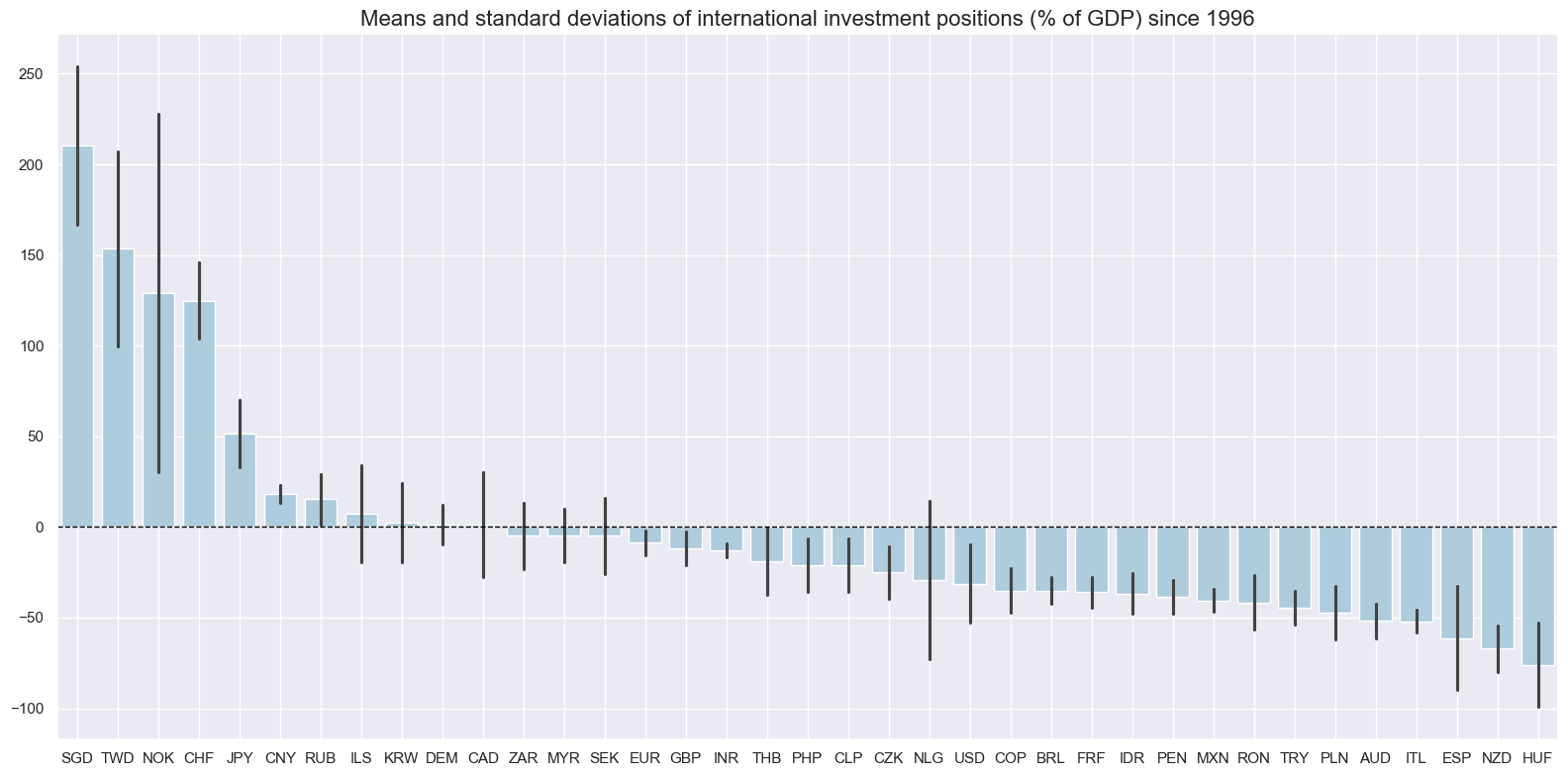
Average net international investment positions since the mid-1990s have ranged from net assets of over 200% of GDP in Singapore to a net liabilities of roughly 70% of GDP in Hungary.

xcatx = ["NIIPGDP_NSA"]
cidx = cids_exp
start_date = "1996-01-01"

msp.view_ranges(
    df,
    xcats=xcatx,
    cids=cidx,
    sort_cids_by="mean",
    start=start_date,
    kind="bar",
    size=(16, 8),
    title="Means and standard deviations of international investment positions (% of GDP) since 1996",
)

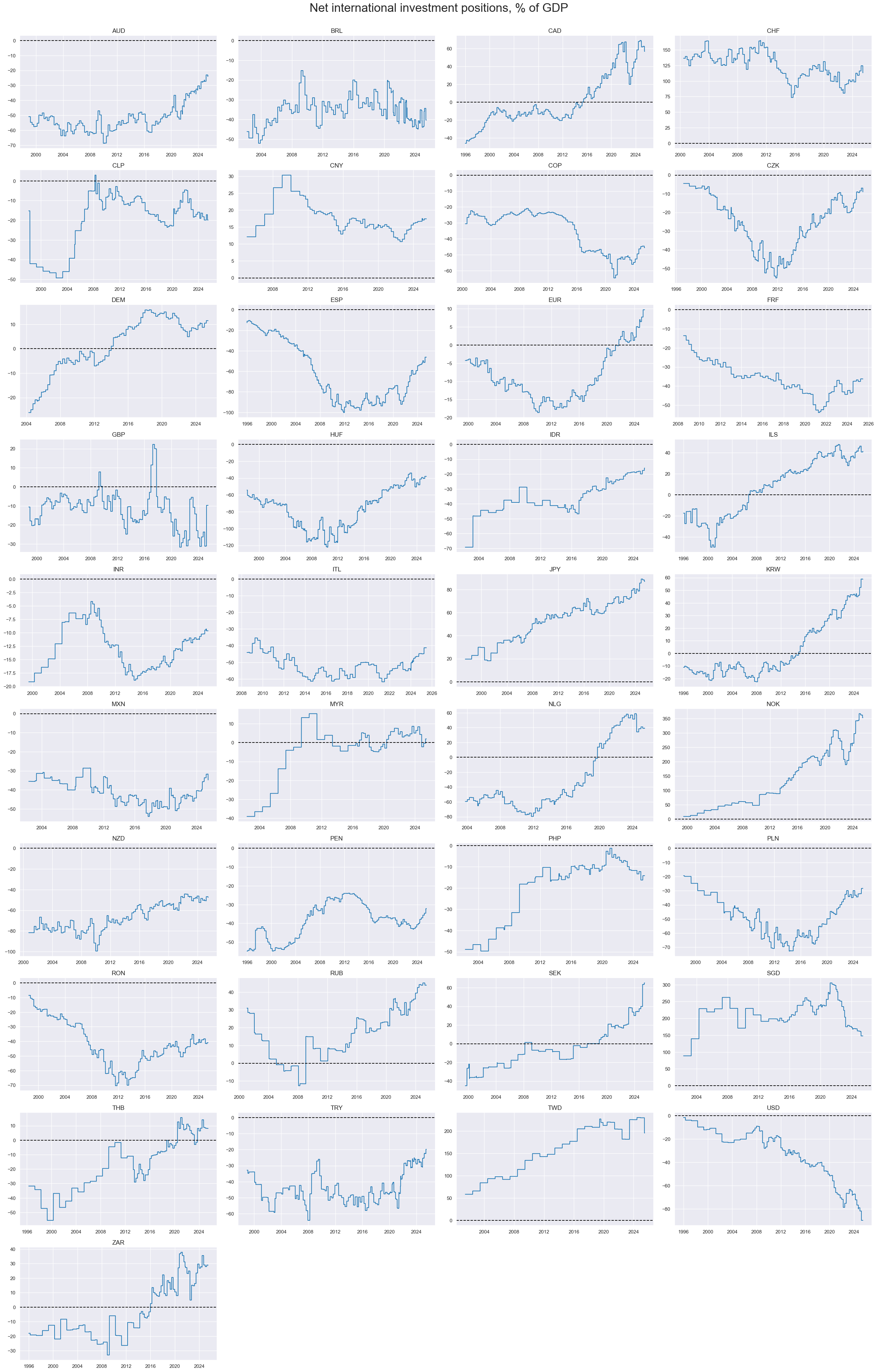
Changes in net international investment positions often come in multi-year trends. Norway, Taiwan and Singapore stand out in terms of increases in net assets as ratio to GDP over the past 20 years.

xcatx = ["NIIPGDP_NSA"]
cidx = cids_exp 
start_date = "1996-01-01"

msp.view_timelines(
    df,
    xcats=xcatx,
    cids=cidx,
    start=start_date,
    title="Net international investment positions, % of GDP",
    title_fontsize=27,
    ncol=4,
    same_y=False,
    size=(16, 8),
    all_xticks=True,
)

xcatx = ["NIIPGDP_NSA"]
cidx = cids_frontier 
start_date = "1996-01-01"

msp.view_timelines(
    df,
    xcats=xcatx,
    cids=cidx,
    start=start_date,
    title="Net international investment positions, % of GDP, frontier markets",
    title_fontsize=27,
    ncol=4,
    same_y=False,
    size=(16, 8),
    all_xticks=True,
)

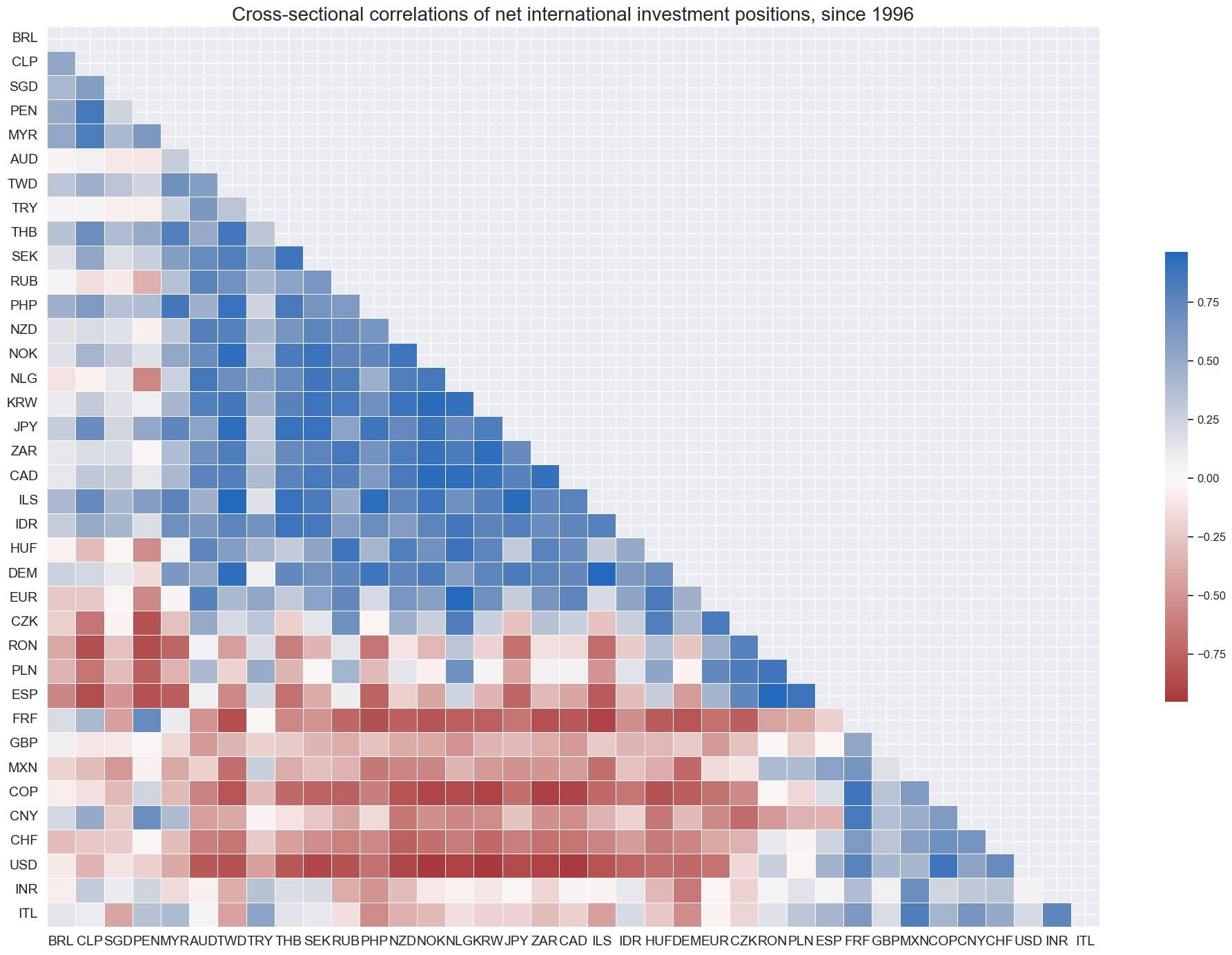
Global correlations of investment positions have been very diverse.

xcatx = ["NIIPGDP_NSA"]
cidx = cids_exp

msp.correl_matrix(
    df,
    xcats=xcatx,
    cids=cidx,
    size=(20, 14),
    cluster=True,
    freq="M",
    title="Cross-sectional correlations of net international investment positions, since 1996",
)

Net international investment position changes

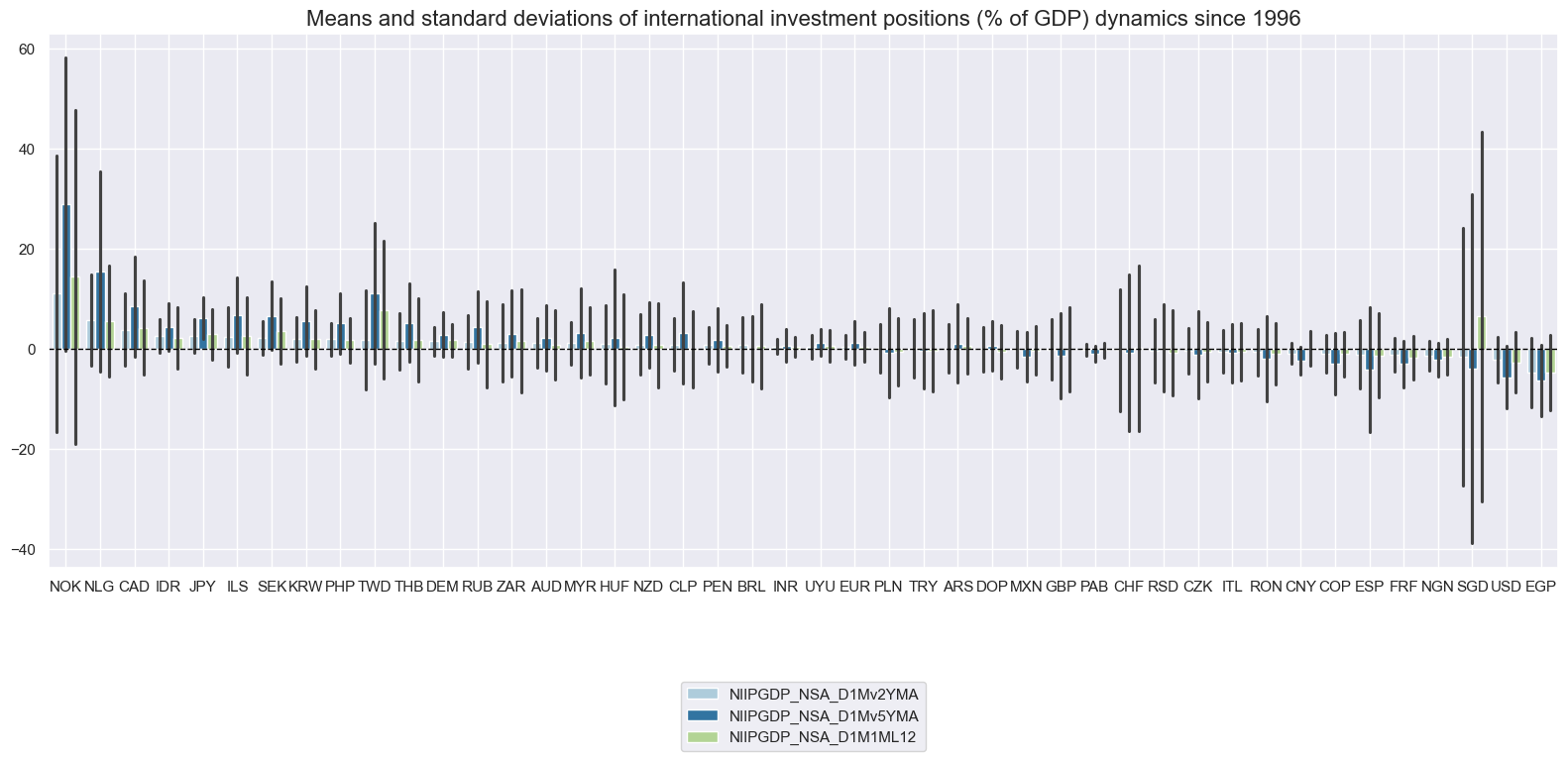
Variation in international investment position ratios is very different across countries. Small open economies with sovereign wealth funds post the largest absolute changes.

xcatx = ["NIIPGDP_NSA_D1Mv2YMA", "NIIPGDP_NSA_D1Mv5YMA", "NIIPGDP_NSA_D1M1ML12"]
cidx = cids
start_date = "1996-01-01"

msp.view_ranges(
    df,
    xcats=xcatx,
    cids=cidx,
    sort_cids_by="mean",
    start=start_date,
    kind="bar",
    size=(16, 8),
    title="Means and standard deviations of international investment positions (% of GDP) dynamics since 1996",
)

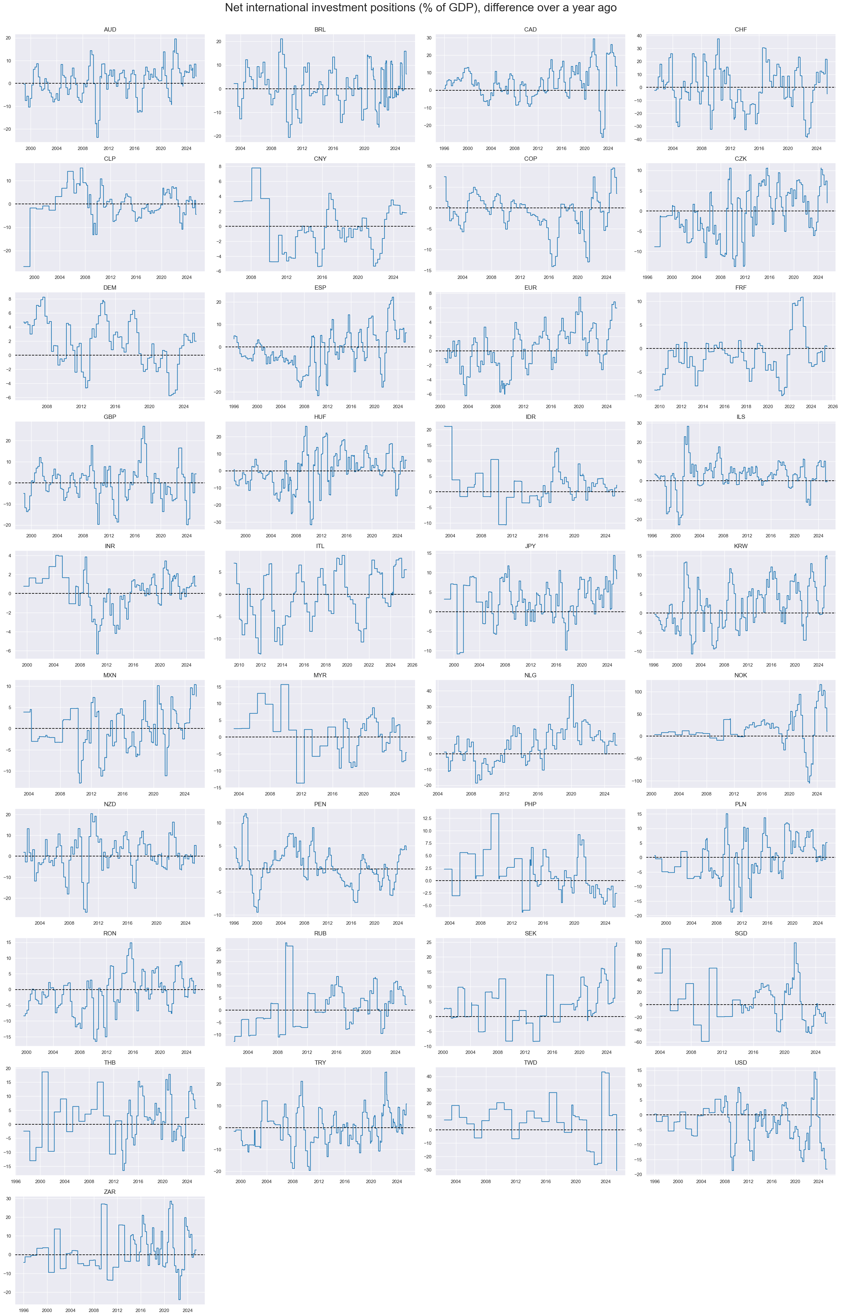
Annual changes in net international investment positions have posted pronounced cycles over the past 25 years, with all countries experiencing both positive and negative changes.

xcatx = ["NIIPGDP_NSA_D1M1ML12"]
cidx = cids_exp
start_date = "1996-01-01"

msp.view_timelines(
    df,
    xcats=xcatx,
    cids=cidx,
    start=start_date,
    title="Net international investment positions (% of GDP), difference over a year ago",
    title_fontsize=27,
    ncol=4,
    same_y=False,
    size=(16, 8),
    all_xticks=True,
)

xcatx = ["NIIPGDP_NSA_D1M1ML12"]
cidx = cids_frontier
start_date = "1996-01-01"

msp.view_timelines(
    df,
    xcats=xcatx,
    cids=cidx,
    start=start_date,
    title="Net international investment positions (% of GDP), difference over a year ago, frontier markets",
    title_fontsize=27,
    ncol=4,
    same_y=False,
    size=(16, 8),
    all_xticks=True,
)

International liabilities as % of GDP

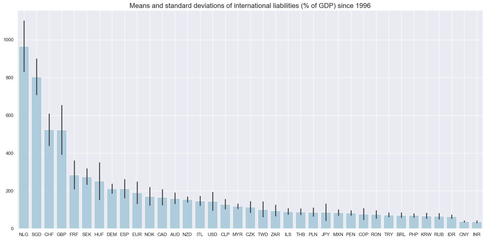
International liabilities are semi-structural indicators. Countries with disproportionately large financial centers have the largest international liabilities as ratio of GDP. Developed countries and small countries also tend to have greater liabilities.

xcatx = ["IIPLIABGDP_NSA"]
cidx = cids_exp
start_date = "1996-01-01"

msp.view_ranges(
    df,
    xcats=xcatx,
    cids=cidx,
    sort_cids_by="mean",
    start=start_date,
    kind="bar",
    size=(16, 8),
    title="Means and standard deviations of international liabilities (% of GDP) since 1996",
)

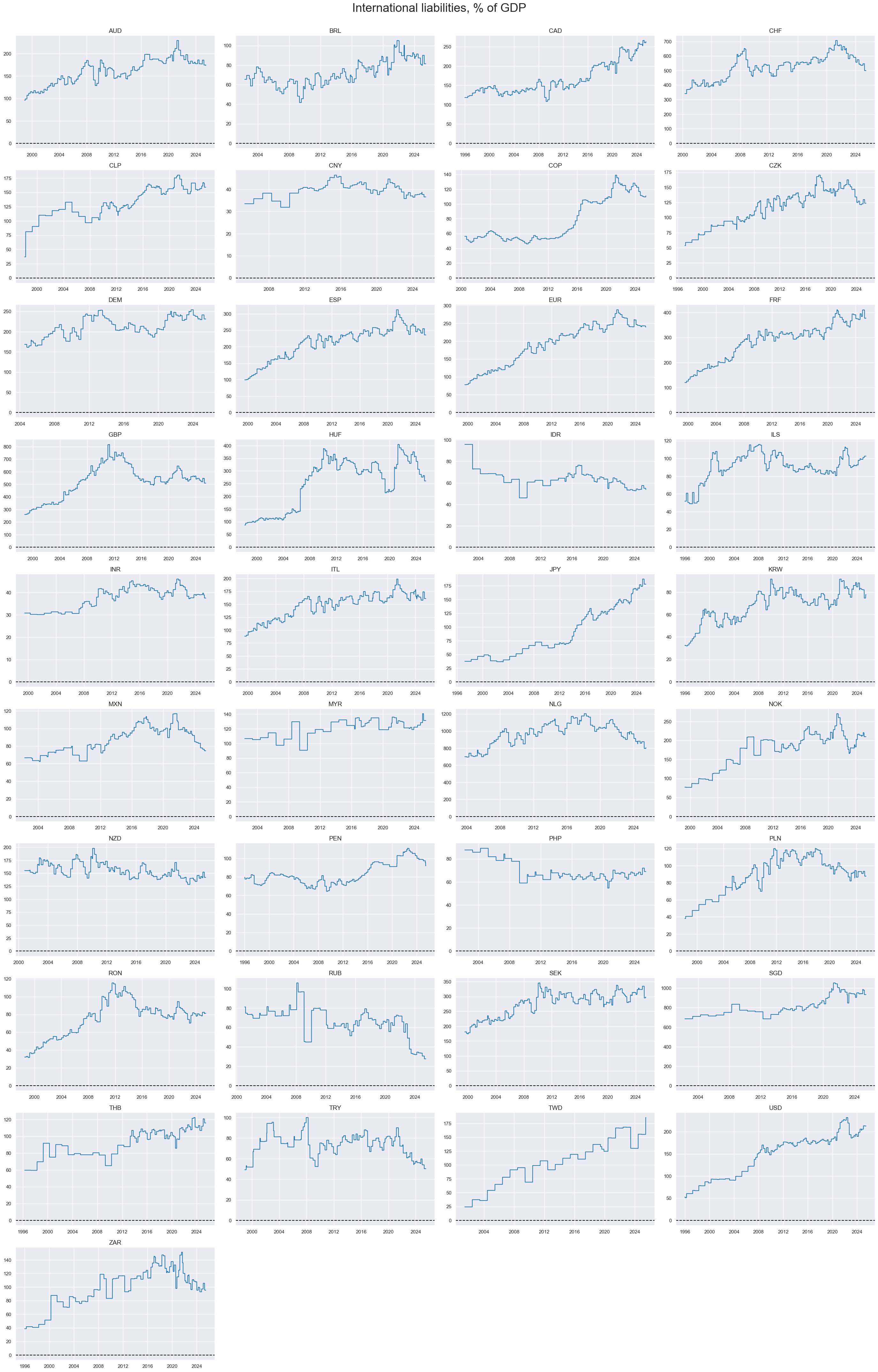
International liabilities as ratios to GDP have not typically been stationary since the mid-1990s but rather trending upward, indicative of the growth of international finance.

Great Britain, Switzerland and Singapore stand out in terms of accumulation of international liabilities as % of GDP over the last 30 years.

xcatx = ["IIPLIABGDP_NSA"]
cidx = cids_exp
start_date = "1996-01-01"

msp.view_timelines(
    df,
    xcats=xcatx,
    cids=cidx,
    start=start_date,
    title="International liabilities, % of GDP",
    title_fontsize=27,
    xcat_labels=["International liabilities"],
    ncol=4,
    same_y=False,
    size=(16, 8),
    all_xticks=True,
)

xcatx = ["IIPLIABGDP_NSA"]
cidx = cids_frontier
start_date = "1996-01-01"

msp.view_timelines(
    df,
    xcats=xcatx,
    cids=cidx,
    start=start_date,
    title="International liabilities, % of GDP, frontier markets",
    title_fontsize=27,
    xcat_labels=["International liabilities"],
    ncol=4,
    same_y=False,
    size=(16, 8),
    all_xticks=True,
)

International liabilities as % of GDP dynamics

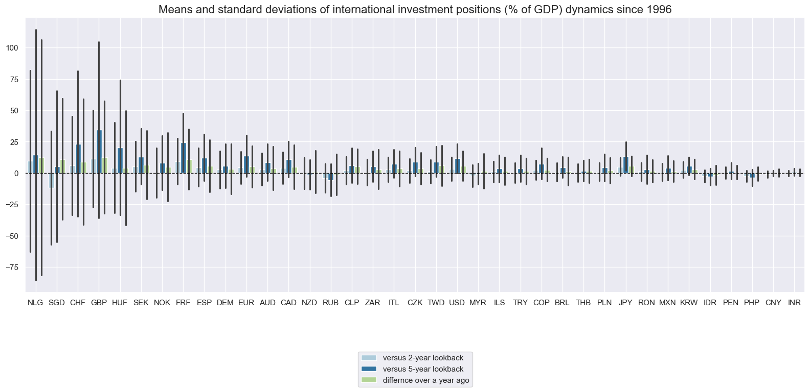
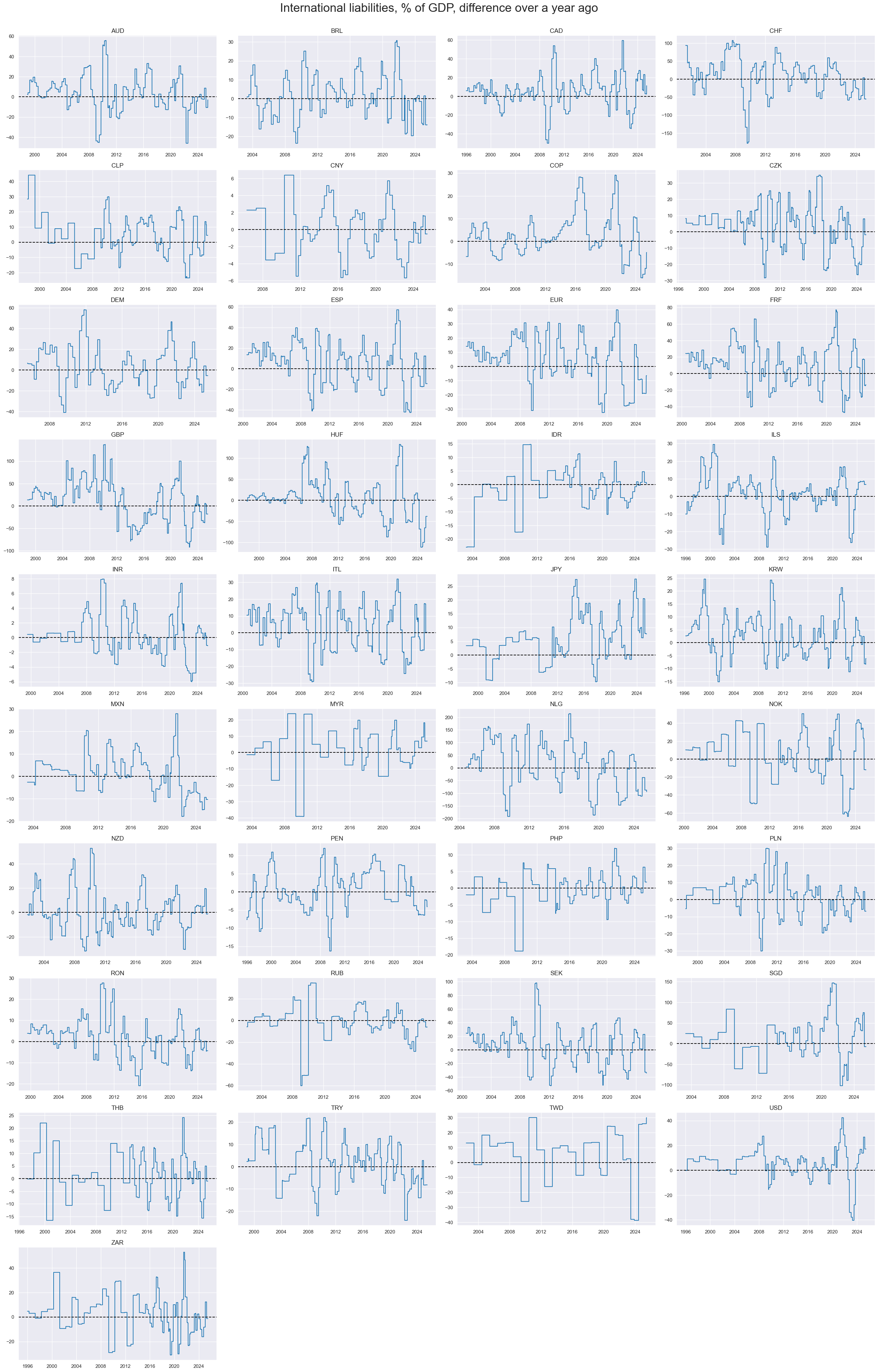
Liability dynamics are very heteroskedastic. Small countries with large financial centers have experienced the most volatile liability dynamics.

xcatx = ["IIPLIABGDP_NSA_D1Mv2YMA", "IIPLIABGDP_NSA_D1Mv5YMA", "IIPLIABGDP_NSA_D1M1ML12"]
cidx = cids_exp
start_date = "1996-01-01"

msp.view_ranges(
    df,
    xcats=xcatx,
    cids=cidx,
    sort_cids_by="std",
    start=start_date,
    kind="bar",
    size=(16, 8),
    title="Means and standard deviations of international investment positions (% of GDP) dynamics since 1996",
        xcat_labels =["versus 2-year lookback","versus 5-year lookback", "differnce over a year ago"]
)

Liability accumulation typically experiences pronounced cycles, with all countries experiencing both positive and negative changes.

xcatx = ["IIPLIABGDP_NSA_D1M1ML12"]
cidx = cids_exp
start_date = "1996-01-01"

msp.view_timelines(
    df,
    xcats=xcatx,
    cids=cidx,
    start=start_date,
    title="International liabilities, % of GDP, difference over a year ago",
    title_fontsize=27,
    ncol=4,
    same_y=False,
    size=(16, 8),
    all_xticks=True,
)

xcatx = ["IIPLIABGDP_NSA_D1M1ML12"]
cidx = cids_frontier
start_date = "1996-01-01"

msp.view_timelines(
    df,
    xcats=xcatx,
    cids=cidx,
    start=start_date,
    title="International liabilities, % of GDP, difference over a year ago, frontier markets",
    title_fontsize=27,
    ncol=4,
    same_y=False,
    size=(16, 8),
    all_xticks=True,
)

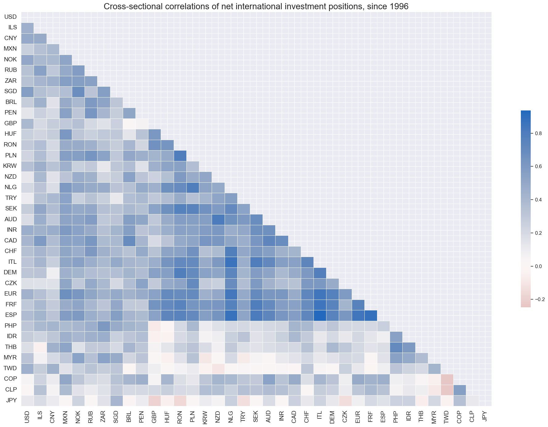
Changes in liabilities have been correlated internationally.

xcatx = ["IIPLIABGDP_NSA_D1M1ML12"]
cidx = cids_exp

msp.correl_matrix(
    df,
    xcats=xcatx,
    cids=cidx,
    size=(20, 14),
    cluster=True,
    freq="M",
    title="Cross-sectional correlations of net international investment positions, since 1996",
)

Importance

Research links

On IIP and external crisis likelihood/ CDS spreads:

“Using a sample of 73 advanced and emerging economies and new database on the IIP’s currency composition, we find that the size and structure of external liabilities and assets, especially with regards to currency denomination, matter in understanding balance-of-payments pressures. Specifically…higher levels of gross external debt increase the likelihood of an external crisis, while higher levels of foreign-currency-denominated external debt increase the likelihood of sudden stops.” Cubeddu, Hannan and Rabana

“… the size and currency composition of the IIP matters, especially for EMDEs (emerging market and developing economies): higher external debt increases the likelihood of external crises, while higher foreign currency-denominated debt increases the likelihood of sudden stops. Official reserves act as a mitigating factor by reducing the probability of external crises, with diminishing returns…” Cubeddu, Hannan and Rabana

“… we find that the ratio of net foreign liabilities to GDP is a significant crisis predictor…” GM Milesi-Ferretti, L Catão

On IIP and FX returns:

“Macro trading factors for FX must foremostly consider (gross) external investment positions. That is because modern international capital flows are mainly about financing, i.e. exchanges of money and financial assets, rather than saving, real investments and consumption (which are goods market concepts). Trades in financial assets are much larger than physical resource trades. Also, financing flows simultaneously create aggregate purchasing power, bank assets and liabilities. The vulnerability of currencies depends on gross rather than net external debt. Current account balances, which indicate current net payment flows, can be misleading. The nature and gravity of financial inflow shocks, physical saving shocks, credit shocks and – most importantly – ‘sudden stops’ all depend critically on international financing.” Macrosynergy

“A deterioration of a country’s NFA (net foreign asset) to GDP position tends to have the largest depreciating exchange rate effects (both nominal and real) when domestic inflation significantly exceeds inflation abroad.” M Binder

“… it was found that an increase of the IIP GL (Grubel and Lloyd) index also had effects on the trajectory of the exchange rate, as a shock in the IIP promoted devaluation of the domestic currency [in Brazil].” PR Vartanian et al

Empirical Clues

Identifying and isolating periods characterized by official exchange rate targets, illiquidity, or convertibility-related distortions in FX markets is crucial for testing any FX-based hypothesis. These periods can significantly influence the behavior and dynamics of currency markets, and neglecting to account for them can result in inaccurate or misleading conclusions. Therefore, we compile a blacklist of such periods for all cross-sections to ensure accurate analysis.

dfb = df[df["xcat"].isin(["FXTARGETED_NSA", "FXUNTRADABLE_NSA"])].loc[
    :, ["cid", "xcat", "real_date", "value"]
]
dfba = (
    dfb.groupby(["cid", "real_date"])
    .aggregate(value=pd.NamedAgg(column="value", aggfunc="max"))
    .reset_index()
)
dfba["xcat"] = "FXBLACK"
fxblack = msp.make_blacklist(
    dfba, "FXBLACK"
)  # exclude periods of FX targeting or illiquidity

dfx=df.copy()

International liabilities trend and local currency bond index returns

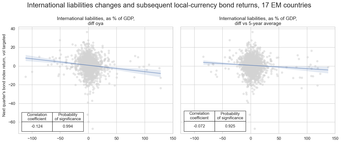
The rapid accumulation of foreign liabilities is an indicator of overborrowing and vulnerability to tightening global financial conditions. Conversely, a rapid reduction in foreign liabilities is an indicator of deleveraging and a potential improvement in the country’s creditworthiness.

Indeed, there has been strong and significant negative relationships between the trend in international liabilities and subsequent local currency bond index excess returns. The relationship holds across all measures of the trend but has been most pronounced for the annual change in liabilities.

xcatx = ["IIPLIABGDP_NSA_D1M1ML12", "IIPLIABGDP_NSA_D1Mv5YMA"]

no_bonds = ["ILS", "INR", "KRW", "SGD", "TWD"]  # countries with insufficient local bond data
cidx= list(set(cids_em) - set(no_bonds)) 

cr = {}

for sig in xcatx:
    cr[f"cr_{sig}"] = msp.CategoryRelations(
        dfx,
        xcats=[sig, "LCBIXR_VT10"],
        cids=cidx,
        freq="q",
        lag=1,
        xcat_aggs=["last", "sum"],
        start="2000-01-01",
        blacklist=fxblack,
    )

# Combine all CategoryRelations instances for plotting
all_cr_instances = [
    cr[f"cr_{sig}"] for sig in xcatx 
]

# Define easy-to-read labels for the signals
xlab_dict = {
     "IIPLIABGDP_NSA_D1M1ML12": "International liabilities, as % of GDP, diff oya", 
     "IIPLIABGDP_NSA_D1Mv5YMA": "International liabilities, as % of GDP, diff vs 5-year average", 
 }

# Define all labels for the subplot titles
all_labels = [
    f"{sig}" for sig in xlab_dict.values() 
]


msv.multiple_reg_scatter(
    cat_rels=all_cr_instances,
    title="International liabilities changes and subsequent local-currency bond returns, 17 EM countries",
    ylab="Next quarter's bond index return, vol targeted",
    ncol=2,
    nrow=1,  
    figsize=(14, 6),
    prob_est="map",
    coef_box="lower left",
    subplot_titles=all_labels,
)

LCBIXR_VT10 misses: ['ARS', 'DOP', 'PAB', 'UYU'].
LCBIXR_VT10 misses: ['ARS', 'DOP', 'PAB', 'UYU'].

International liabilities trends and FX forward returns

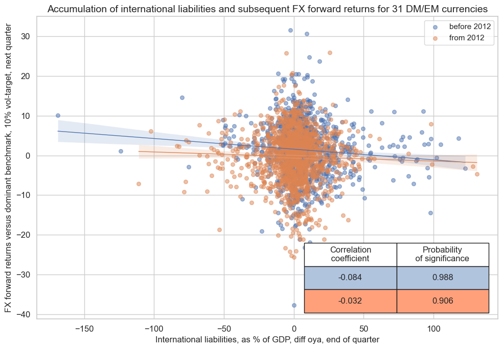
The accumulation of international liabilities also increases the risk of currency depreciation. Indeed, there has been a strong and significant negative relationship between the trend in international liabilities and subsequent FX forward returns in both developed and emerging markets.

xcatx = ["IIPLIABGDP_NSA_D1M1ML12", "FXXR_VT10"]
cidx = cids_exp

cr = msp.CategoryRelations(
    dfx,
    xcats=xcatx,
    cids=cidx,
    freq="q",
    lag=1,
    xcat_aggs=["mean", "sum"],
    start="2000-01-01",
    blacklist=fxblack,
)

cr.reg_scatter(
    coef_box="lower right",
    prob_est="map",
    separator=2012,
    title="Accumulation of international liabilities and subsequent FX forward returns for 31 DM/EM currencies",
    xlab="International liabilities, as % of GDP, diff oya, end of quarter",
    ylab="FX forward returns versus dominant benchmark, 10% vol-target, next quarter",
    size=(10, 7),
)

FXXR_VT10 misses: ['USD'].

International liabilities trends and CDS returns

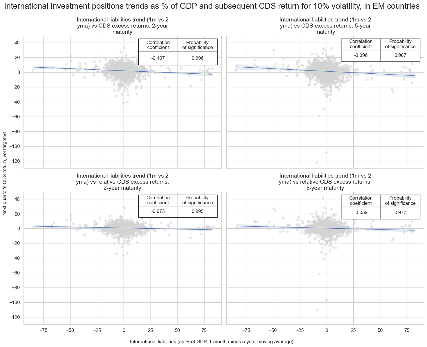
There is pervasive evidence of a negative relationship between the international liabilities trend and subsequent CDS returns in emerging markets. The relationship has been significant for both relative and directional returns.

xcatx = ["CDS02YXR_VT10", "CDS05YXR_VT10"]

dfa = msp.make_relative_value(
    dfx,
    xcats=xcatx,
    cids=cids,
    rel_xcats=[xc + "vGLB" for xc in xcatx],
)
dfx = msm.update_df(dfx, dfa)

The category, CDS02YXR_VT10, is missing ['TWD', 'NGN', 'UYU', 'EGP', 'RSD', 'DOP', 'EUR', 'NLG', 'INR', 'PAB', 'CAD', 'ARS', 'SGD'] from the requested basket. The new basket will be ['AUD', 'BRL', 'CHF', 'CLP', 'CNY', 'COP', 'CZK', 'DEM', 'ESP', 'FRF', 'GBP', 'HUF', 'IDR', 'ILS', 'ITL', 'JPY', 'KRW', 'MXN', 'MYR', 'NOK', 'NZD', 'PEN', 'PHP', 'PLN', 'RON', 'RUB', 'SEK', 'THB', 'TRY', 'USD', 'ZAR'].

# Define the target categories

targs = ["CDS02YXR_VT10", "CDS05YXR_VT10", "CDS02YXR_VT10vGLB", "CDS05YXR_VT10vGLB"]

targs_dict = {
    "CDS02YXR_VT10": "CDS excess returns: 2-year maturity",
    "CDS05YXR_VT10": "CDS excess returns: 5-year maturity",
    "CDS02YXR_VT10vGLB": "relative CDS excess returns: 2-year maturity", 
    "CDS05YXR_VT10vGLB": "relative CDS excess returns: 5-year maturity"
}

xcatx = ["IIPLIABGDP_NSA_D1Mv2YMA"]

cidx= list(set(cids_em) - set(['INR', 'SGD', 'TWD']) - set(cids_frontier)) # all available EM countries for CDS returns

# Define easy-to-read labels for the signals
xlab_dict = {
    "IIPLIABGDP_NSA_D1Mv2YMA": "International liabilities trend (1m vs 2 yma)",
    
   }

# Initialize the dictionary to store CategoryRelations instances
cr = {}

# Loop through the signals and target categories
for sig in xcatx:
    for targ in targs:
        cr[f"cr_{sig}_{targ}"] = msp.CategoryRelations(
            dfx,
            xcats=[sig, targ],
            cids=cidx,
            freq="Q",
            lag=1,
            xcat_aggs=["last", "sum"],
            start="2000-01-01",
            blacklist=fxblack,
        )

# Combine all CategoryRelations instances for plotting
all_cr_instances = [
    cr[f"cr_{sig}_{targ}"] for sig in xcatx for targ in targs
]

# Define all labels for the subplot titles
all_labels = [
    f"{sig} vs {targ}" for sig in xlab_dict.values() for targ in targs_dict.values()
]

# Plotting the results
msv.multiple_reg_scatter(
    cat_rels=all_cr_instances,
    title="International investment positions trends as % of GDP and subsequent CDS return for 10% volatility, in EM countries",
    ylab="Next quarter's CDS return, vol targeted",
    xlab= "International liabilities (as % of GDP, 1-month minus 5-year moving average)",
    ncol=2,
    nrow=len(all_labels) // 2,  # Adjust the number of rows based on the number of plots,
    figsize=(15, 12),
    prob_est="map",
    coef_box="upper right",
    subplot_titles=all_labels,
)

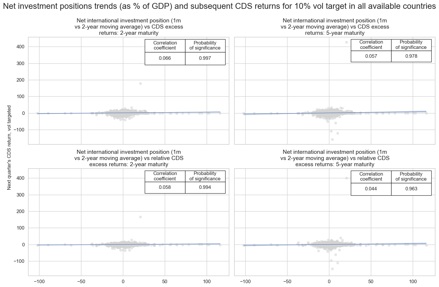
There is pervasive evidence of a positive relation between net international investment position trend and subsequent CDS returns for all available countries. The relationship has been significant for both relative and directional returns.

# Define the target categories
targs = ["CDS02YXR_VT10", "CDS05YXR_VT10", "CDS02YXR_VT10vGLB", "CDS05YXR_VT10vGLB"]

targs_dict = {
    "CDS02YXR_VT10": "CDS excess returns: 2-year maturity",
    "CDS05YXR_VT10": "CDS excess returns: 5-year maturity",
    "CDS02YXR_VT10vGLB": "relative CDS excess returns: 2-year maturity", 
    "CDS05YXR_VT10vGLB": "relative CDS excess returns: 5-year maturity"
}

xcatx = ["NIIPGDP_NSA_D1M1ML12"]

cidx= list(set(cids_exp) - set(['INR', 'SGD', 'TWD', 'CAD', 'EUR']) - set(cids_frontier)) # all available countries for CDS returns

# Define easy-to-read labels for the signals
xlab_dict = {
     "NIIPGDP_NSA_D1M1ML12": "Net international investment position (1m vs 2-year moving average)"
}

# Initialize the dictionary to store CategoryRelations instances
cr = {}

# Loop through the signals and target categories
for sig in xcatx:
    for targ in targs:
        cr[f"cr_{sig}_{targ}"] = msp.CategoryRelations(
            dfx,
            xcats=[sig, targ],
            cids=cidx,
            freq="q",
            lag=1,
            xcat_aggs=["last", "sum"],
            start="2000-01-01",
            blacklist=fxblack,
        )

# Combine all CategoryRelations instances for plotting
all_cr_instances = [
    cr[f"cr_{sig}_{targ}"] for sig in xcatx for targ in targs
]

# Define all labels for the subplot titles
all_labels = [
    f"{sig} vs {targ}" for sig in xlab_dict.values() for targ in targs_dict.values()
]

# Plotting the results
msv.multiple_reg_scatter(
    cat_rels=all_cr_instances,
    title="Net investment positions trends (as % of GDP) and subsequent CDS returns for 10% vol target in all available countries",
    ylab="Next quarter's CDS return, vol targeted",
    ncol=2,
    nrow=len(all_labels) // 2,  # Adjust the number of rows based on the number of plots,
    figsize=(15, 10),
    prob_est="map",
    coef_box="upper right",
    subplot_titles=all_labels,
)

Net international investment position and international liabilities ratios vs local real interest rates

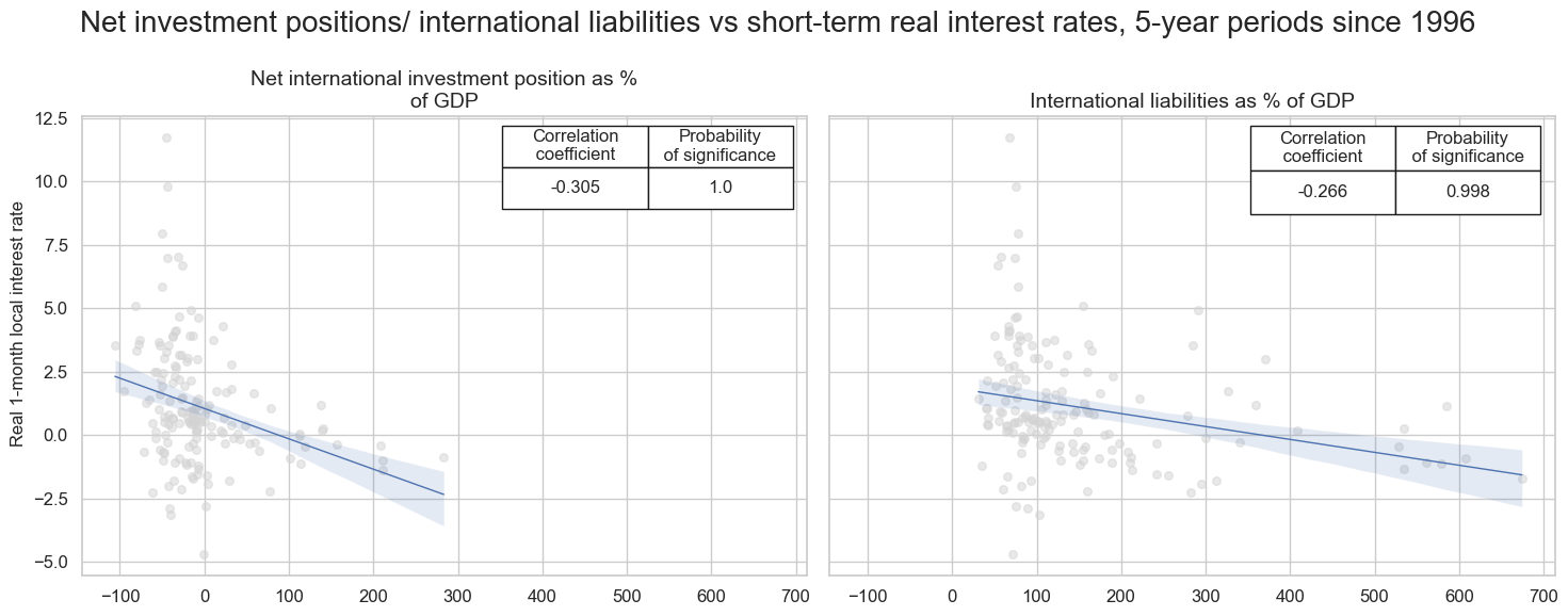
There has been a negative correlation between net international investment position/ international liabilities ratios and local real interest rates. Short-term real interest rates tend to be lower in countries with larger net external assets (such as Norway, Singapore, Switzerland and Taiwan), probably because those countries tend to keep local rates low, in order to discourage additional capital inflows in order to prevent excessive exchange rate strength.

xcatx = ["NIIPGDP_NSA", "IIPLIABGDP_NSA"]
xlab_dict = {
    "NIIPGDP_NSA": "Net international investment position as % of GDP", 
    "IIPLIABGDP_NSAA": "International liabilities as % of GDP",
   }
cidx = cids_exp
start_date = "1996-01-01"

cr = {}

for sig in xcatx:
    cr[f"cr_{sig}"] = msp.CategoryRelations(
        dfx,
        xcats=[sig, "RIR_NSA"],
        cids=cidx,
        freq="M",
        lag=0,
        xcat_aggs=["mean", "mean"],
        start=start_date,
        years=5,
        blacklist=fxblack,
        )

# Combine all CategoryRelations instances for plotting
all_cr_instances = [
    cr[f"cr_{sig}"] for sig in xcatx
]

# Define all labels for the subplot titles
all_labels = [
    f"{sig}" 
    for sig in xlab_dict.values()
]

msv.multiple_reg_scatter(
    cat_rels=all_cr_instances,
    title="Net investment positions/ international liabilities vs short-term real interest rates, 5-year periods since 1996",
    ylab="Real 1-month local interest rate",
    ncol=2,
    nrow=len(all_labels) // 2,  # Adjust the number of rows based on the number of plots,
    figsize=(15, 6),
    prob_est="map",
    coef_box="upper right",
    subplot_titles=all_labels,
)

Appendices

Appendix 1: Currency symbols

The word ‘cross-section’ refers to currencies, currency areas or economic areas. In alphabetical order, these are AED (Emirates dirham), ARS (Argentine Peso), AUD (Australian dollar), BRL (Brazilian real), CAD (Canadian dollar), CHF (Swiss franc), CLP (Chilean peso), CNY (Chinese yuan renminbi), COP (Colombian peso), CZK (Czech Republic koruna), DEM (German mark), DOP (Dominican Peso), EGP (Egyptian Pound), ESP (Spanish peseta), EUR (Euro), FRF (French franc), GBP (British pound), HKD (Hong Kong dollar), HUF (Hungarian forint), IDR (Indonesian rupiah), ITL (Italian lira), JPY (Japanese yen), KRW (Korean won), MXN (Mexican peso), MYR (Malaysian ringgit), NGN (Nigerian Naira), NLG (Dutch guilder), NOK (Norwegian krone), NZD (New Zealand dollar), OMR (Omani Rial), PAB (Panamanian balboa), PEN (Peruvian sol), PHP (Phillipine peso), PLN (Polish zloty), QAR (Qatari riyal), RON (Romanian leu), RSD (Serbian Dinar), RUB (Russian ruble), SAR (Saudi riyal), SEK (Swedish krona), SGD (Singaporean dollar), THB (Thai baht), TRY (Turkish lira), TWD (Taiwanese dollar), USD (U.S. dollar), UYU (Uruguayan peso), VEF (Venezuelan bolívar), ZAR (South African rand).