Machine learning for international trading strategies

Jupyter Notebook

Financial markets’ broadening access to point-in-time economic indicators across countries offers a robust foundation for diversified international trading strategies. The central challenge lies in combining multiple macro factors into a single positioning signal for each country—drawing on statistical patterns from both global and country-specific (local) experiences. To address this, we propose a novel “global-local” method of machine learning for generating international macro trading signals. This method manages the bias-variance tradeoff by regularizing country-level coefficients toward their global counterparts. Crucially, the strength of this regularization diminishes when historical evidence supports the value of emphasizing local relationships over global ones. We demonstrate the approach by applying it to international equity index futures strategies. The “global-local” method has generated stronger predictive power and higher risk-adjusted returns than either fully country-specific models or globally pooled alternatives.

The post below is based on Macrosynergy’s proprietary research. Please quote as “Gholkar, Rushil and Sueppel, Ralph, ‘Machine learning for international trading strategies,’ Macrosynergy research post, July 2025.”

A Jupyter notebook for auditing and replicating the research results can be downloaded here. The notebook operation requires access to J.P. Morgan DataQuery to download data from JPMaQS. Everyone with DataQuery access can download data except for the latest months. Moreover, J.P. Morgan offers free trials on the complete dataset for institutional clients. An academic support program sponsors data sets for research projects.

International trading strategies and the bias-variance trade-off

The increased scope of point-in-time macro-quantamental data enables the construction of ample, valid macro factors for trading strategies. The critical challenge has become selecting and combining candidate factors. This article focuses particularly on the construction of international macro trading signals. Generally, macro trading signals are quantitative instructions for positions in financial markets based on macroeconomic information. International refers to the consideration of multiple currency areas for the purpose of one strategy; we backtest and trade the same factors across several markets. The cross-country approach not only offers diversification but also allows for combining the diverse and comparative experiences when drawing empirical lessons. Machine learning with international data optimizes model parameters and hyperparameters by sequentially using point-in-time panels, i.e., datasets spanning multiple currency areas and time periods. This approach is suitable for realistic backtests and has been explained in a previous post (Macro trading signal optimization: basic statistical learning methods).

As elsewhere, the success of machine learning with international data depends on managing its bias-variance trade-off, i.e., balancing method simplicity and flexibility. Bias refers to errors that result from oversimplification. Variance refers to errors that result from excessive sensitivity to changes in the trading data. For international macro trading strategies, this trade-off is a critical consideration:

• The bias-variance trade-off is steep: The historic experience of the relation between low-frequency economic trends and financial returns in modern markets is limited to a few decades. Typically, data series become painfully short if we wish to train and test models from the early 2000s or the 1990s onward. This means that every inch of freedom granted to a learning method typically comes at a high price in terms of variance. This generally calls for parsimonious models and is a key motivation for using international panel data in the first place.
• Cross-country diversity is evident: Assuming all countries to be equal in terms of the relation between macro factors and returns means that related model would be biased (albeit this may be acceptable). The degree to which we model structural differences across countries is crucial for striking a balance between simplicity and flexibility. On the simplistic end of the spectrum are panel models that apply equal coefficients for all factors across all countries. On the flexible end are country-specific models that estimate coefficients based solely on the country experience.

Previous posts by Macrosynergy on panel-based machine learning have all chosen the simple panel regression method, accepting high bias to reduce variance. However, as time series lengthen, more flexible models become feasible. Additionally, there is clear evidence of relevant structural diversity in currency areas that influence how economic information impacts returns. Such diversity arises from economic structures, monetary policy regimes, and data quality. With sufficient available data, the choice between simple panel models and more flexible country models might thus be delegated to the statistical learning process itself.

The “global-local” method

We propose a statistical learning method that estimates coefficients in an international data set by considering both global and country-specific relations. The globally pooled and country models are set as the extreme points in the bias-variance trade-off. Intuitively speaking, the global pooled model utilizes a broad and diverse set of data, including cross-country differences in feature and return data, but allows only global coefficients, i.e., one coefficient size fits all countries. By contrast, individual country models allow for diverse local coefficients, but derive these only through local data, disregarding the information provided by the rest of the panel.

The “global-local” method works by regularization, shrinking country-specific (“local”) coefficients towards their pooled (“global”) values. The degree of shrinkage depends on the size of the penalty imposed on the relative local coefficient. The penalty hyperparameter at each point in time is determined through statistical learning, specifically through optimizing predictive power in cross-validation, using the sample to date. If the penalty grows with the square of the local coefficient, as in the case of Ridge regressions, the “global local” method effectively follows a theoretical prior that local coefficients are normally distributed around a global mean with unknown standard deviation. The smaller the standard deviation, the stronger the effective regularization and the greater the importance of global versus local estimates.

Technically, the “global-local” method estimates global and local coefficients simultaneously by minimizing mean squared errors, while applying penalties to both absolute and relative coefficient sizes. First, it penalizes the deviation between local and global coefficients using the L2 norm—i.e., in proportion to the square of their differences—weighted by a penalty parameter (local_lambda). This parameter is typically selected through cross-validation during the machine learning process. Second, the method applies an additional L2 penalty to the global coefficients themselves, akin to Ridge regression, controlled by a separate parameter (global_lambda), also determined via statistical learning. The global-local method is implemented in the GlobalLocalRegression class of the Macrosynergy package.

This “global-local” method can be embedded in a sequential machine learning process in Python that uses scikit-learn and related functions of the Macrosynergy package, and which is divided into five steps:

1. Collect features (factor candidates) and targets (returns of traded positions) at the frequency that is suitable for the learning process and in the form of double-indexed pandas data frames. The frequency will be monthly in all examples below.
2. Define model and hyperparameter grids in scikit-learn style. These define the model versions over which the statistical learning process optimizes based on cross-validation within expanding samples. One of these hyperparameters will be the penalty parameter for the local coefficients’ deviations from the global coefficients.
3. Specify time series panel splits for sequential cross-validation using a specialized function of the Macrosynergy package. Here, we use the ExpandingKFoldPanelSplit splitter, a panel data analogue of scikit-learn’s TimeSeriesSplit splitter, which divides the panel by dates into sequential and non-overlapping intervals.
4. Set an appropriate optimization criterion for cross-validation. In this post, we only use the mean-squared error criterion, which is easily comparable across global and local models.
5. Optimize models and signals sequentially for the eligible history, i.e., from the earliest start date with sufficient data to the present. This can be managed efficiently by using the SignalOptimizer Python class. The optimization process of this class compares and selects models prior to each rebalancing date, delivers related optimal signals, and enables visualization of the optimization process over time. The sequentially optimized signals provide a valid basis for backtesting the overall strategy process, eliminating biases arising from hindsight.

Empirical example: international equity futures trading

In this post, we apply the global-local method to cross-country equity futures strategies driven by macro-quantamental factors. The goal is to outperform passive or static allocations by dynamically managing exposure to local-currency equity futures across time and markets. Machine learning is used to assign weights to twelve plausible point-in-time conceptual factor scores, combining them into a single positioning signal. Each conceptual factor represents a coherent economic theme—such as inflation—and is constructed from a set of normalized, point-in-time macroeconomic indicators that jointly capture the underlying concept.

We selected 18 local-currency equity index futures for analysis, based on their liquidity and the availability of point-in-time macroeconomic factors. These contracts cover eight developed markets and ten emerging market stock indices. The developed markets (in order of currency tickers) are Australia (AUD), Canada (CAD), Switzerland (CHF), the euro area (EUR), the UK (GBP), Japan (JPY), Sweden (SEK), and the U.S. (USD). The emerging markets are Brazil (BRL), South Korea (KRW), Mexico (MXN), Malaysia (MYR), Poland (PLN), Singapore (SGD), Thailand (THB), Taiwan (TWD), Turkey (TRY), and South Africa (ZAR). For a detailed list of the actual stock indices, see Annex 1 below.

For all selected countries and equity markets, we compute twelve conceptual macro factor scores. These scores logically group low-level macro-quantamental indicators into broader, more abstract economic concepts. Typically, macro-quantamental scores are normalized values of economic indicators, expressed relative to their neutral levels, with standard deviations calculated based on a cross-section of comparable countries up to the current point in time. Conceptual factor scores are then constructed as sequentially re-normalized combinations of macro-quantamental scores that capture similar economic themes.

To maintain consistency, we generally define these concepts such that their theoretical effect on target returns is negative; hence, some of the slightly unconventional names. All conceptual factors and their underlying macro-quantamental inputs are detailed in Annex 2. A brief and intuitive summary is provided below:

• Domestic spending growth shortfall measures (negative) country expenditure in excess of medium-term GDP growth and central bank targets. Soft domestic spending typically warrants policy support.
• Inflation shortfall ratios measure (negative) scaled differences between inflation trends and central bank targets. Sub-par inflation encourages easy monetary policy.
• Intervention liquidity growth measures changes in estimated central bank (base) money injections in the economy associated with FX interventions or security purchases and tends to push equity values higher.
• Real yield shortfalls measure the shortfall of interest rates in relation to labor productivity. Lower real interest rates increase the net present value of future profits.
• External balance ratios include external trade, current account, and net FDI balances relative to GDP. External surpluses often indicate undervalued currencies, competitive economies, and future local liquidity growth.
• External balance changes are trends in external current account balances and merchandise trade balances. Shifts toward surplus often indicate improving competitiveness and local liquidity conditions.
• Labor market slackening measures the weakening in local labor market conditions, heralding easing wage cost pressure and easier monetary conditions.
• Effective currency depreciation here refers to recent dynamics in trade-weighted exchange rates. Recent effective depreciation is expected to lead to increases in reported local earnings from exports and foreign subsidiaries.
• Terms-of-trade improvement measures commodity-based import-export price dynamics. Improving terms of trade indicate higher corporate profitability and increased investment activity in the local economy.
• Excess money growth uses narrow and broad money growth in excess of medium-term GDP growth and central bank targets. A rapidly rising stock of deposits at banks often increases the odds of larger flows into equity markets in the near future.
• Business “gloom” means low business confidence survey readings. Evidence of such gloom may indicate higher equity risk premia and increase the chances of policy support for the corporate sector.
• Short-term business confidence improvement measures short-term changes in business survey levels. These changes bode well for near-term profitability, while not yet significantly affecting monetary policy.

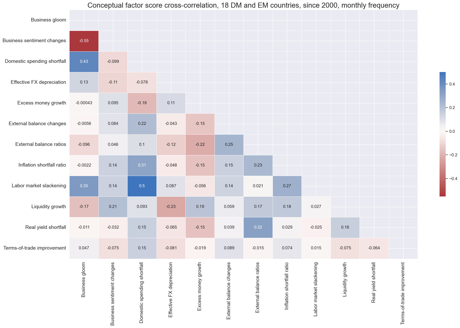
The annotated matrix below displays the Pearson correlation coefficients of the twelve conceptual factor scores at a monthly frequency for a panel of 18 countries since 2000. There have been some factors with a larger positive correlation, particularly domestic spending shortfall, business gloom, and labor market slack, all of which are related to the state of the business cycle. Additionally, there has been a strong negative correlation between business gloom and improvements in business sentiment. Otherwise, correlations have been modest and diverse, suggesting that, for the most part, conceptual differences also translate into statistical differences.

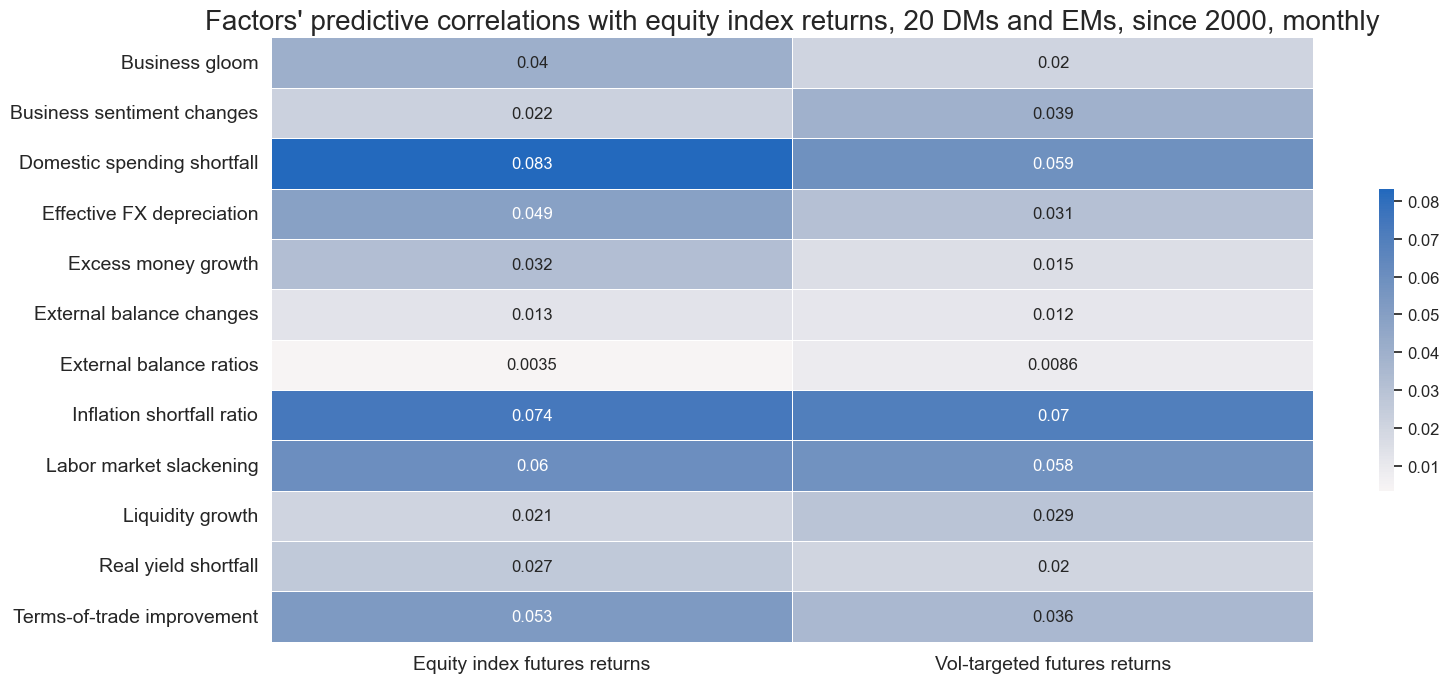
The graph below illustrates the predictive correlations between the macro factor scores’ information states at the end of the month and the local equity index’s future returns (both outright and volatility-targeted) during the next month. All predictive correlations have been positive, confirming standard theoretical priors and hinting at some information inefficiency in financial markets, although some coefficients have been very small.

Empirical evidence

The purpose of this section is to compare the predictive power and trading value of signals based on three machine learning methods:

• Sequential machine learning with pooled regression.
• Sequential machine learning with country regressions.
• Sequential machine learning with the “global-local” method.

All methods use the above 14 conceptual macro factors. The targets of the machine learning process are volatility-targeted equity index futures returns for all countries. Volatility targeting means that positions are scaled based on past volatility, such that the expected annualized return on the underlying risk capital is 10%. The adjustment reduces the dominance of high-volatility periods in cross-validation.

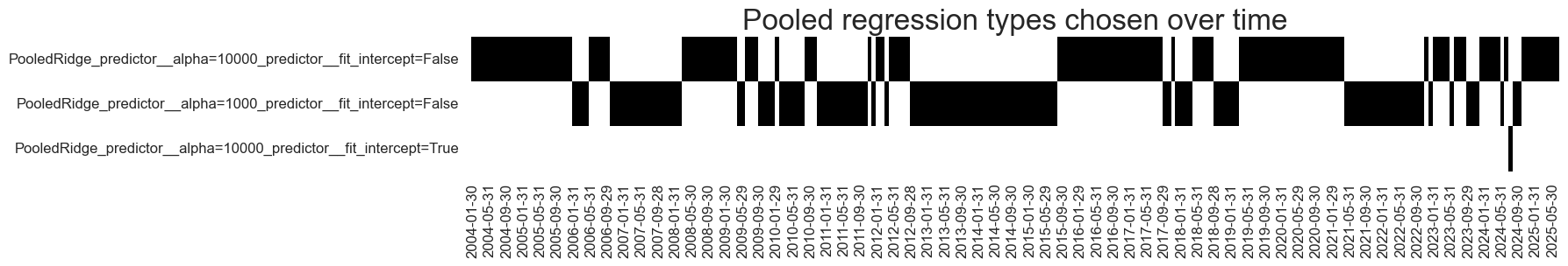
Pooled regression-based learning is the high-bias, low-variance path. We use regularized regressions of the Ridge type, which penalize the squared values of the coefficients of standardized factors. The hyperparameters to be determined by cross-validation include the penalty factor and the inclusion of an intercept. This means that the learning process decides sequentially the strength of regularization and the consideration of a long or short bias in the signal, relative to the factor score values. With data available for most countries dating back to 2000, sequential learning can be employed only from 2004. Since then, the learning process has generally preferred aggressive regularization with high penalty parameters (alphas), ranging from 1000 to 10,000, out of a range of 1 to 10,000.

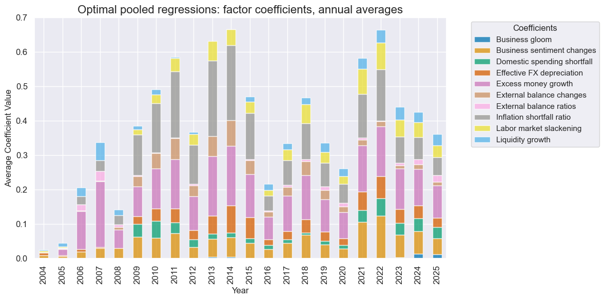
The coefficients of normalized factor scores are indicative of the importance of the respective economic concepts. The absolute size of coefficients varies over time, partly due to variations in regularization strength. Towards the end of the sample, the most important concepts for predicting local equity returns were excess money growth, improvements in business sentiment, and inflation shortfall ratios. Also, labor market slack, domestic spending shortfall, liquidity growth, and effective currency depreciation played a noticeable role.

The learning process based on country regressions also utilizes Ridge regressions, with the same hyperparameters that we offered to the pooled regressions. Again, the process mostly chose highly regularized regressions as optimal and rarely added an intercept to the model.

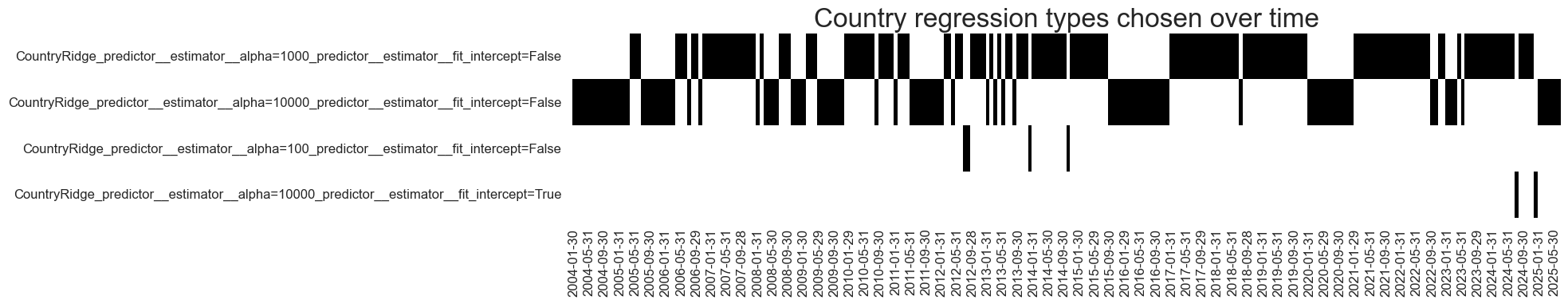
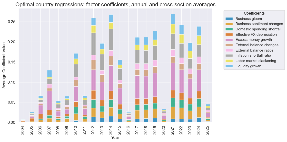
The variation of coefficient sizes was even more conspicuous for country regressions, presumably due to their greater sensitivity to new data and changes in regularization strength. The relative importance of conceptual factors towards the end of the sample was similar to the pooled regression case, however.

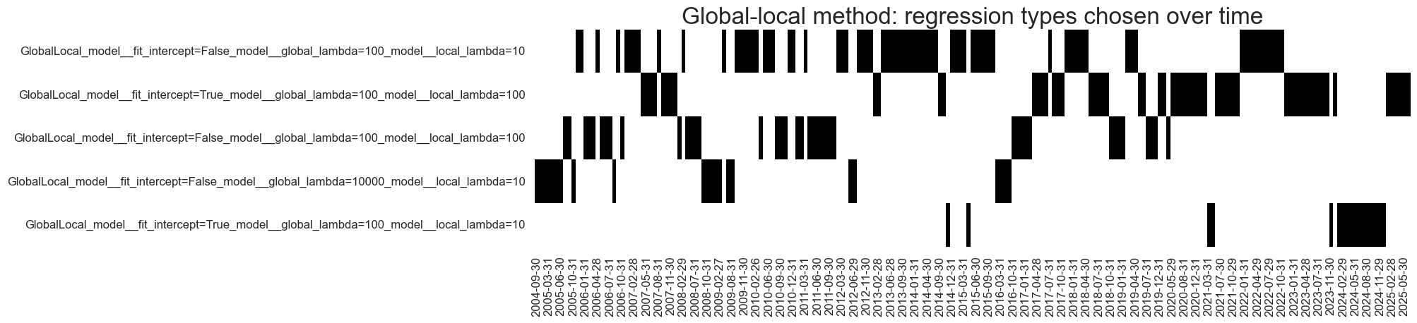
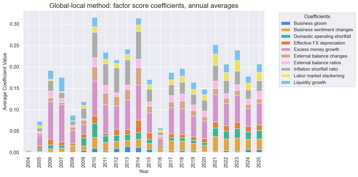
The “global-local” method, which combines pooled (global) and country (local) coefficients by regularizing the local coefficients towards the global ones and global coefficients towards zero. The regularization of the local coefficients has been mild. The regularization of the global coefficients has been somewhat more aggressive, but not as assertive as in the cases of pooled and country regressions.

The relative importance of global macro factors in predicting equity returns towards the end of the sample has been similar to that of the pooled global regression-based process.

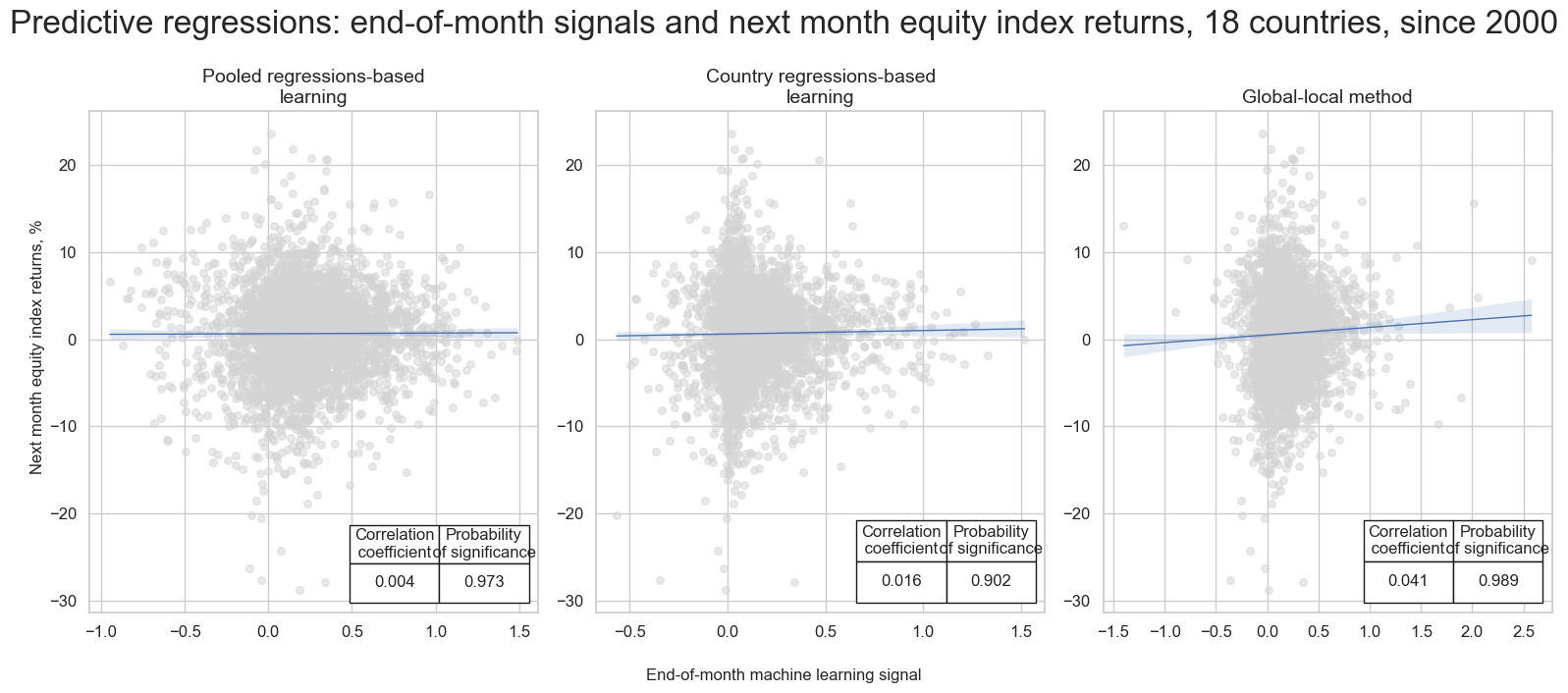
The regression scatterplots below compare the predictive relation between end-of-month signals and next-month equity returns as generated by the three methods. The key finding is that the signals generated by the global-local method showed the strongest and most significant predictive power for subsequent equity index returns across countries and over time. Non-parametric correlation analysis based on Kendall metrics confirms that finding.

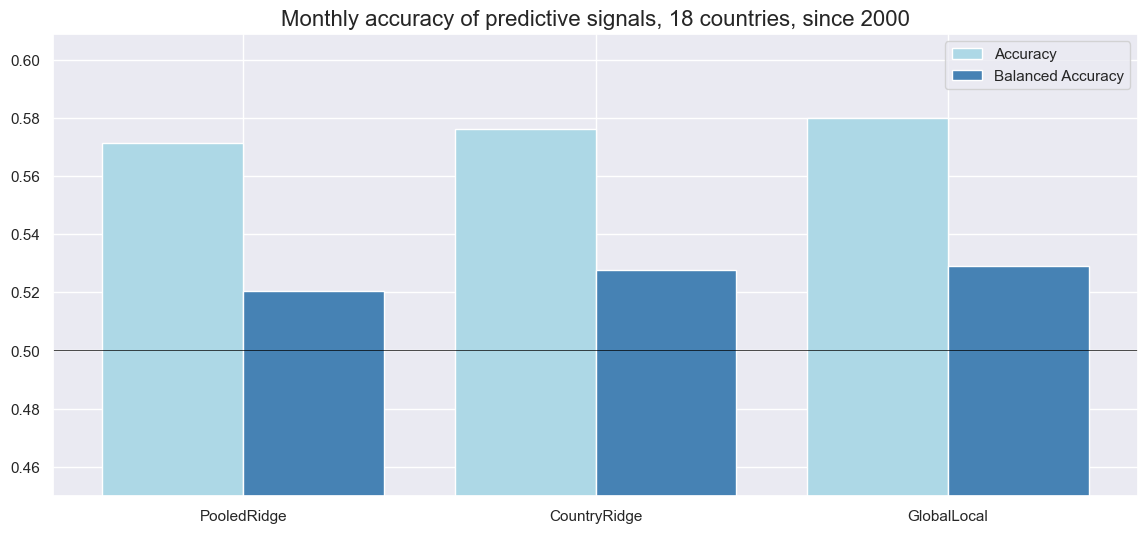
Also, monthly accuracy, i.e., the ratio of correctly predicted signs of monthly returns, has been highest for the “global-local” method, at around 58%. However, balanced accuracy —the average of correctly predicted positive and negative returns —has been equal for both the pooled and “global-local” methods.

We assess the economic value of the machine learning signals for various types of naïve profit and loss statements (PnLs). Naïve PnLs followed a standard methodology applied in many Macrosynergy posts. Here, they utilize month-end signals generated by the above learning processes to instruct position-taking at the beginning of the next month, assuming a one-day delay between signal calculation and the completion of position changes. The naïve PnLs do not consider transaction costs or compounding. For the simulations below, all PnLs have been scaled to an annualized volatility of 10%, for ease of comparison of risk-adjusted returns.

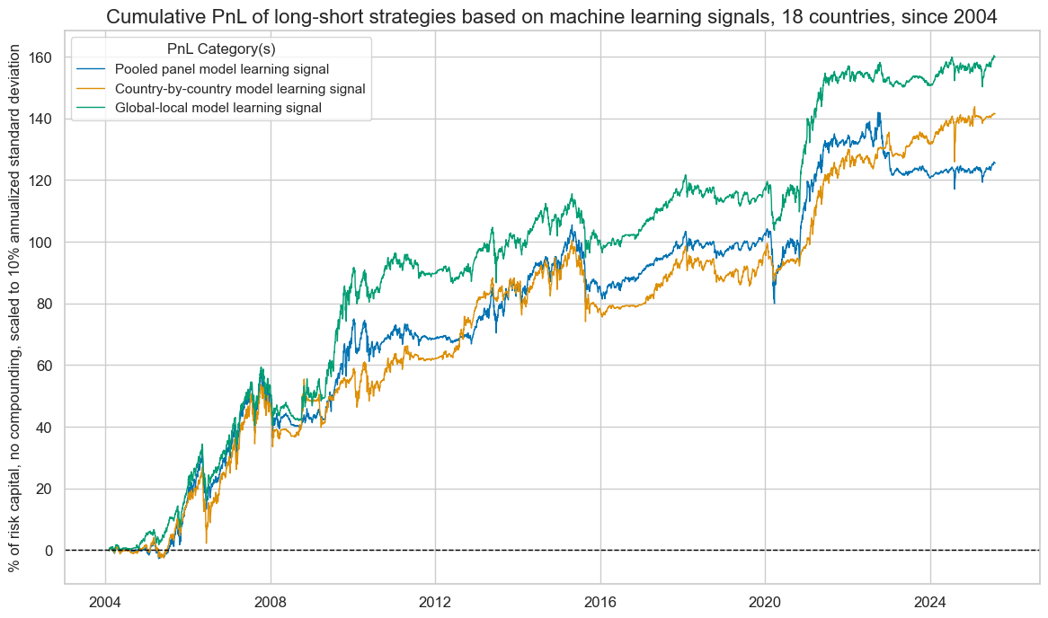
The first naïve PnL is for a long-short equity futures strategy that takes independent positions across all local equity index futures in accordance with normalized local signals that contain values at three standard deviations on the positive and negative sides. This strategy does not have an explicit structural long bias in equity; however, it has had an implicit long bias since 2004, due to favorable macroeconomic conditions, including low inflation and the aggressive expansion of central bank liquidity. The basis of value generation of a long-short strategy is the management of direction and strength of equity market exposure across countries. All machine learning signals have produced positive long-term risk-adjusted returns, but the performance metrics of the “global-local” method have been superior. The pooled and country models’ signals have produced Sharpe ratios of 0.6 and Sortino ratios of 0.8-0.9. The “global-local” method’s signals would have produced a long-term Sharpe ratio of 0.7-0.8 and a Sortino ratio of 1.0-1.1. All strategies recorded daily correlation with S&P500 futures returns of around 30%.

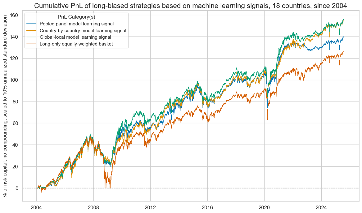
The second PnL corresponds to a long-biased equity futures strategy. The long bias is introduced by adding one standard deviation to the normalized signals across all 18 markets, with values capped at three standard deviations. Value generation in this strategy stems from actively managing overall equity risk exposure, including through occasional short positions, and its allocation across countries.

The long bias yields similar overall performances in terms of Sharpe and Sortino ratios, but with higher S&P 500 correlations of around 55%. Also, the advantage of the “global-local” method has been less clear, outperforming the pooled regressions-based method but not the country regressions-based method by much. All machine-learning-based signals have outperformed the long-only strategy that takes equally sized positions in all futures.

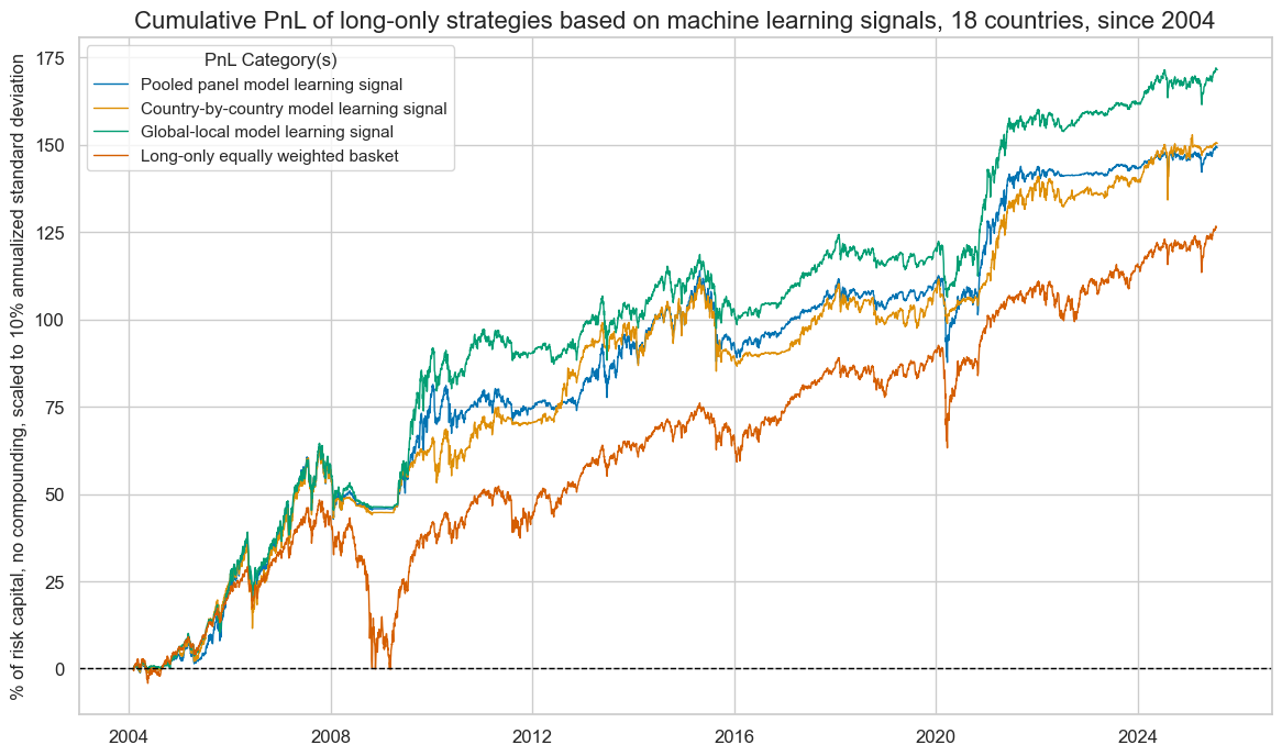
A final test for the economic value of the various machine learning-generated composite macro signals is the PnLs of long-only equity futures strategies. These signals are truncated versions of the original machine learning signals that do not allow short positions. All value generation relies on cross-sectional and intertemporal allocation of equity exposure. The “global-local” signals have produced the highest risk-adjusted value, with a long-term Sharpe of 0.8 and a long-term Sortino ratio of 1.1. Again, all learning-based signals have outperformed the equally weighted long-only portfolio in risk adjusted terms.

Annex 1: Local-currency equity index futures

This post looks at eight developed market local-currency index futures and ten emerging market local-currency index futures. The developed market indices are (in alphabetical order of currency symbol):

• AUD: The S&P/ASX 200 is the primary index for the Australian equity market. It measures the performance of the 200 largest companies by market capitalization listed on the Australian Stock Exchange (ASX).
• CAD: The S&P/TSX 60 Index is designed to represent the large-cap segment of the Canadian equity market. It includes 60 of the largest and most liquid companies listed on the Toronto Stock Exchange (TSX).
• CHF: The Swiss Market Index (SMI) is Switzerland’s premier stock market index, representing the 20 largest and most liquid companies listed on the SIX Swiss Exchange.
• EUR: The EURO STOXX 50 Index is a leading stock market index for the euro area, representing the 50 largest and most liquid blue-chip companies from 11 Eurozone countries.
• GBP: The FTSE 100 Index is a stock market index representing the 100 largest publicly listed companies by market capitalization on the London Stock Exchange (LSE).
• JPY: The Nikkei 225 Stock Average Index is a prominent stock market index in Japan, representing 225 of the largest and most liquid companies listed on the Tokyo Stock Exchange (TSE).
• SEK: The OMX Stockholm 30 (OMXS30) Index is a major stock market index in Sweden, representing the 30 most traded large-cap companies listed on the Nasdaq Stockholm exchange.
• USD: The S&P 500 Composite Index is one of the most widely followed stock market indices in the world, representing 500 of the largest publicly traded companies in the United States. (Note that even though the U.S. is about twice the size of the euro area, the market capitalization of the S&P500 has been roughly ten times that of EURO STOXX.)

The emerging market indices are:

• BRL: The Brazil Bovespa Index, also known as the Ibovespa is the main stock market index in Brazil, representing the performance of the most actively traded companies on the B3, the São Paulo Stock Exchange.
• KRW: The KOSPI 200 Index is a major stock market index in South Korea, representing the performance of the 200 largest and most liquid companies listed on the Korea Exchange (KRX).
• MXN: The Mexico IPC, often referred to as the Bolsa Index, is the main stock market index in Mexico. It tracks the performance of the 35 largest and most liquid companies listed on the Mexican Stock Exchange.
• MYR: The FTSE Bursa Malaysia KLCI (Kuala Lumpur Composite Index) is the main stock market index in Malaysia. It tracks the performance of the 30 largest companies by market capitalization listed on the Bursa Malaysia
• PLN: The Warsaw General Index 20 comprises the 20 largest and most liquid companies listed on the Warsaw Stock Exchange (WSE) in Poland.
• SGD: The MSCI Singapore (Free) Index represents the performance of the Singapore equity market through a free float-adjusted market capitalization-weighted index.
• THB: The Bangkok SET 50 Index is a major stock market index in Thailand, representing the 50 largest companies listed on the Stock Exchange of Thailand.
• TWD: The Taiwan Stock Exchange Weighted Index (TAIEX) is the main stock market index in Taiwan. It tracks the performance of all listed companies on the Taiwan Stock Exchange.
• TRY: The BIST 30 Index is one of the leading stock market indices of Turkey, tracking the 30 largest and most liquid companies listed on Borsa Istanbul.
• ZAR: The FTSE/JSE Top 40 Index is a key stock market index in South Africa, representing the 40 largest companies listed on the Johannesburg Stock Exchange (JSE) by market capitalization.

Annex 2: Conceptual macro factor scores

The conceptual macro factor scores of this post are sequentially re-normalized composite scores based on quantamental indicator scores, as detailed below.

• Domestic spending growth shortfall measures (negative) country expenditure in excess of medium-term GDP growth and central bank targets. Excess domestic spending encourages tightening of monetary policy. The underlying quantamental indicators are 6-month/6-month and annual import trends (documentation here) as well as annual nominal retail sales growth (documentation here), real retail sales growth (documentation here) and real private consumption growth (documentation here), all in excess of a 5-year moving median of annual real GDP growth (documentation here) and, for nominal quantities, a central bank target (documentation here).
• Inflation shortfall ratios measure (negative) scaled differences between inflation trends and central bank targets. Excess inflation warrants tightening of monetary policy. The underlying quantamental indicators are 6-month/6-month and annual core and headline inflation trends (documentation here), in excess of a central bank target. To make high- and low-inflation country shortfalls comparable, inflation-target differentials are expressed as ratios of effective inflation targets or a minimum of 2%.
• Intervention liquidity growth measures changes in estimated central bank (base) money injections in the economy associated with FX interventions or security purchases. Quantitative easing leads to a fall in interest rates, reducing borrowing and debt-servicing costs for businesses. The underlying quantamental indicators are 3-month and 6-month changes in intervention liquidity as a ratio to GDP (documentation here).
• Negative excess real interest rates measure the shortfall of interest rates in relation to labor productivity. Low real interest rates support demand for capital and the value of existing companies. The underlying quantamental indicators are 1-month real interest rates and both 3-year and 5-year real bond yields (documentation here) in excess of a 5-year moving median in annual real GDP growth minus a 5-year moving median in annual work force growth (documentation here).
• External balance ratios include external current account balances, basic external balances and merchandise trade balances. External surpluses often indicate undervalued currencies, competitive economies or faster local liquidity growth, as central banks stem currency strength through unsterilized interventions. The underlying quantamental indicators are 3-month moving averages in basic external balances-to-GDP ratios (documentation here), current account-to-GDP ratios (documentation here) and merchandise trade balance-to-GDP ratios (documentation here).
• External balance changes are trends in external current account balances and merchandise trade balances. Shifts toward surplus often indicate improving competitiveness and local liquidity conditions. The underlying quantamental indicators are 3-month changes in the 3-month moving average of current account-to-GDP ratio and merchandise trade balance-to-GDP ratio (documentation here) as well as the difference between 3-month moving average and 5-year moving average in the previous external balance ratios (documentation here).
• Labor market slackening measures the weakening in local labor market conditions. Labor market slack typically invites local monetary policy support for financial markets. The underlying quantamental indicators are annual changes in unemployment rate (documentation here) and the (negative) 3-month moving average of 1-year employment growth (documentation here) in excess of the 5-year moving median in annual work force growth.
• Effective currency depreciation here refers to recent dynamics in trade-weighted exchange rates. Recent effective depreciation bodes for increases in reported local earnings from exports and foreign subsidiaries. The underlying quantamental indicators are annual trends in openness-adjusted effective real and nominal appreciation (documentation here) as well as unadjusted real effective appreciation (documentation here).
• Terms-of-trade improvement measures commodity-based import-export price dynamics. Improving terms of trade point to higher corporate profitability and investment activity in the local economy. The underlying quantamental indicators are percent changes of the latest month over a year ago and percent changes of the latest month over previous 12-months’ average (documentation here).
• Excess money growth uses narrow and broad money growth in excess of medium-term GDP growth and central bank targets. A rapidly rising stock of deposits at banks often increases the odds of larger flows into equity markets. The underlying quantamental indicators are seasonally- and jump-adjusted annual narrow (documentation here) and broad money growth (documentation here) in excess of a 5-year moving median in annual real GDP growth and central bank targets.
• Business “gloom” means low business confidence survey readings. Evidence of such gloom may indicate higher equity risk premia and increases the chances of policy support for the corporate sector. Underlying quantamental indicators are z-scores of manufacturing (documentation here), services (documentation here) and construction confidence (documentation here) survey scores and associated 3-month moving averages. 4/9ths of the combination is placed on each of manufacturing and services industries, with 1/9th weight on construction.
• Short-term business confidence improvement measures short-term changes in business survey levels. These changes bode well for near-term profitability, while not yet affecting monetary policy so much. The underlying quantamental indicators are 3-month and 6-month changes in manufacturing (documentation here), services (documentation here) and construction confidence (documentation here), with 4/9ths of weight placed equally on manufacturing and services sectors, with 1/9th weight on construction.