Monetary aggregates

This category group contains information states of growth and trends of nominal and real monetary aggregates. Monetary aggregates are banking system liabilities that at least partly function similar to traditional money. We use two definitions “narrow”, which is close to the concept of M1, and “broad”, which usually refers to the concept of M3 but in some countries has been preferable to use M2. Money growth can be indicative of liquidity growth, inflation pressure, and economic activity.

Narrow money growth

Ticker : MNARROW_SJA_P1M1ML12 / _P1M1ML12_D1M1ML3 / _P3M3ML3AR / _P6M6ML6AR

Label : Narrow money, seasonally- and jump-adjusted: %oya / %oya, diff over 3m / % 3m/3m ar / % 6m/6m ar

Definition : Narrow money, seasonally- and jump-adjusted: % change over a year ago / % change over a year ago, difference over 3 months / % of latest 3 months over previous 3 months at an annualized rate / % of latest 6 months over previous 6 months at an annualized rate.

Notes :

• Narrow money refers to the national definition of M1. M1 refers to the most liquid forms of money-like assets. All are liabilities of the banking system, including the central bank. Across most countries M1 includes physical currency in circulation, demand deposits that are accessible without restrictions, and, mainly in the past, traveler’s checks. There are some minor differences in the specific instruments included in M1 across countries, reflecting differences in financial systems, institutions, and regulations.

• Seasonal adjustment factors are sequentially estimated as new data are released. This means that a new data vintage is created at every estimation.

• Jump adjustment means that two types of outliers are adjusted for. Firstly, large “spikes” (i.e., two subsequent large moves of the seasonal index in opposite directions) are averaged. The causes for such spikes are often holiday shifts between two months, while the causes for jumps are often methodology changes. Secondly, large one-off jumps in the index are replaced by the local trend. The criteria for adjustment are statistically based on pattern recognition.

Ticker : RMNARROW_SJA_P1M1ML12 / _P1M1ML12_D1M1ML3 / _P3M3ML3AR / _P6M6ML6AR

Label : Real narrow money, seasonally- and jump-adjusted: %oya / %oya, diff over 3m / % 3m/3m ar / % 6m/6m ar

Definition : Real narrow money, seasonally- and jump-adjusted: % change over a year ago / % change over a year ago, difference over 3 months ago / % of latest 3 months over previous 3 months at an annualized rate / % of latest 6 months over previous 6 months at an annualized rate.

Notes :

• Nominal narrow money is deflated by headline CPI to obtain real narrow money.

• See notes on narrow money.

Broad money growth

Ticker : MBROAD_SJA_P1M1ML12 / _P1M1ML12_D1M1ML3 / _P3M3ML3AR / _P6M6ML6AR

Label : Broad money, seasonally- and jump-adjusted: %oya / %oya, diff over 3m / % 3m/3m ar / % 6m/6m ar

Definition : Broad money, seasonally- and jump-adjusted: % change over a year ago / % change over a year ago, difference over 3 months / % of latest 3 months over previous 3 months at an annualized rate / % of latest 6 months over previous 6 months at an annualized rate.

Notes :

• Broad money refers to M3 except for a few currency areas, which do not publish it. These are China (CNY), Israel (ILS), South Korea (KRW), Russia (RUB), Taiwan (TWD), and the United States (USD). In these cases we use M2 instead. Typically, M2 includes everything in M1, and adds savings deposits, time deposits, and money market mutual funds of retail clients. M3 usually includes everything in M2 plus, large time deposits, money market mutual funds of institutional clients, repurchase agreements, eurodollars, and some other still liquid assets.

• Seasonal adjustment factors are sequentially re-estimated as new data are released. This means that a new data vintage is created at every estimation.

• Jump adjustment means that two types of outliers are adjusted for. Firstly, large “spikes” (i.e., two subsequent large moves of the seasonal index in opposite directions) are averaged. The causes for such spikes are often holiday shifts between two months, while the causes for jumps are often methodology changes. Secondly, large one-off jumps in the index are replaced by the local trend. The criteria for adjustment are statistically based on pattern recognition.

Ticker : RMBROAD_SJA_P1M1ML12 / _P1M1ML12_D1M1ML3 / _P3M3ML3AR / _P6M6ML6AR

Label : Real broad money, seasonally- and jump-adjusted: %oya / %oya, diff over 3m / % 3m/3m ar / % 6m/6m ar

Definition : Real broad money, seasonally- and jump-adjusted: % change over a year ago / % change over a year ago, difference over 3 months / % of latest 3 months over previous 3 months at an annualized rate / % of latest 6 months over previous 6 months at an annualized rate.

Notes :

• Nominal narrow money is deflated by headline CPI to obtain real narrow money.

• See notes on broad money.

Imports

Only the standard Python data science packages and the specialized macrosynergy package are needed.

import os
import pandas as pd

import macrosynergy.management as msm
import macrosynergy.panel as msp
import macrosynergy.visuals as msv
from macrosynergy.download import JPMaQSDownload

from datetime import date 

import warnings
warnings.simplefilter("ignore")

The JPMaQS indicators we consider are downloaded using the J.P. Morgan DataQuery API interface within the macrosynergy package. This is done by specifying ticker strings , formed by appending an indicator category code <category> to a currency area code <cross_section> . These constitute the main part of a full quantamental indicator ticker, taking the form DB(JPMAQS,<cross_section>_<category>,<info>) , where <info> denotes the time series of information for the given cross-section and category.

The following types of information are available:

• value giving the latest available values for the indicator

• eop_lag referring to days elapsed since the end of the observation period

• mop_lag referring to the number of days elapsed since the mean observation period

• grade denoting a grade of the observation, giving a metric of real time information quality.

After instantiating the JPMaQSDownload class within the macrosynergy.download module, one can use the download(tickers, start_date, metrics) method to obtain the data. Here tickers is an array of ticker strings, start_date is the first release date to be considered and metrics denotes the types of information requested.

# Cross-sections of interest
cids_dmca = [
    "AUD",
    "CAD",
    "CHF",
    "EUR",
    "GBP",
    "JPY",
    "NOK",
    "NZD",
    "SEK",
    "USD",
]  # DM currency areas
cids_dmec = ["DEM", "ESP", "FRF", "ITL", "NLG"]  # DM euro area countries
cids_latm = ["BRL", "COP", "CLP", "MXN", "PEN"]  # LatAm countries
cids_emea = ["CZK", "HUF", "ILS", "PLN", "RON", "RUB", "TRY", "ZAR"]  # EMEA countries
cids_emas = [
    "CNY",
    "IDR",
    "INR",
    "KRW",
    "MYR",
    "PHP",
    "SGD",
    "THB",
    "TWD",
]  # EM Asia countries (without "HKD")

cids_dm = cids_dmca
cids_em = cids_latm + cids_emea + cids_emas

# Equity-specific lists
cids_dmeq = ["AUD", "CAD", "EUR", "GBP", "JPY", "SEK", "USD"]
cids_emeq = ["INR", "KRW", "MXN", "PLN", "SGD", "THB", "TRY", "TWD", "ZAR"]
cids_eq = cids_dmeq + cids_emeq

cids = sorted(cids_dm + cids_em)

# for FX analysis

cids_dmfx =  ["AUD", "CAD", "CHF", "GBP", "NOK", "NZD", "SEK", "JPY"]
cids_emfx = ["BRL", "COP", "CLP", "MXN", "PEN", "CZK", "HUF",
    "ILS", "PLN", "RON", "RUB", "TRY", "ZAR", "IDR",
    "INR", "KRW", "MYR", "PHP", "THB", "TWD"]
cids_fx = cids_dmfx + cids_emfx

cids_eur = ["CHF", "CZK", "HUF", "NOK", "PLN", "RON", "SEK"]  # trading against EUR
cids_eud = ["GBP", "RUB", "TRY"]  # trading against EUR and USD
cids_usd = list(set(cids_fx) - set(cids_eur + cids_eud))

# Quantamental categories of interest
main = [
    # Real narrow
    "RMNARROW_SJA_P1M1ML12",
    "RMNARROW_SJA_P1M1ML12_D1M1ML3",
    "RMNARROW_SJA_P3M3ML3AR",
    "RMNARROW_SJA_P6M6ML6AR",
    # Nominal narrow
    "MNARROW_SJA_P1M1ML12",
    "MNARROW_SJA_P1M1ML12_D1M1ML3",
    "MNARROW_SJA_P3M3ML3AR",
    "MNARROW_SJA_P6M6ML6AR",
    # Nominal broad
    "MBROAD_SJA_P1M1ML12",
    "MBROAD_SJA_P1M1ML12_D1M1ML3",
    "MBROAD_SJA_P3M3ML3AR",
    "MBROAD_SJA_P6M6ML6AR",
    # Real broad
    "RMBROAD_SJA_P1M1ML12",
    "RMBROAD_SJA_P1M1ML12_D1M1ML3",
    "RMBROAD_SJA_P3M3ML3AR",
    "RMBROAD_SJA_P6M6ML6AR",  
]

# economic context
econ = [
    "CPIH_SA_P1M1ML12",
    "REER_NSA_P1M12ML1" 
]

# market links
mark = [
    "EQXR_VT10",
    "EQXR_NSA",
    "DU05YXR_VT10",
    "FXXR_VT10",
    "FXTARGETED_NSA",
    "FXUNTRADABLE_NSA",
]

xcats = main + econ + mark

# Download series from J.P. Morgan DataQuery by tickers
start_date = "1990-01-01"
tickers = [cid + "_" + xcat for cid in cids for xcat in xcats]
print(f"Maximum number of tickers is {len(tickers)}")

# Retrieve credentials

client_id: str = os.getenv("DQ_CLIENT_ID")
client_secret: str = os.getenv("DQ_CLIENT_SECRET")

# Download from DataQuery

with JPMaQSDownload(client_id=client_id, client_secret=client_secret) as downloader:
    df = downloader.download(
        tickers=tickers,
        start_date=start_date,
        metrics=["value", "eop_lag", "mop_lag", "grading"],
        suppress_warning=True,
        show_progress=True,
        report_time_taken=True,
    )

Maximum number of tickers is 768
Downloading data from JPMaQS.
Timestamp UTC:  2025-07-03 08:59:48
Connection successful!

Requesting data: 100%|██████████| 154/154 [00:35<00:00,  4.34it/s]
Downloading data: 100%|██████████| 154/154 [01:31<00:00,  1.68it/s]

Time taken to download data: 	138.07 seconds.
Some expressions are missing from the downloaded data. Check logger output for complete list.
120 out of 3072 expressions are missing. To download the catalogue of all available expressions and filter the unavailable expressions, set `get_catalogue=True` in the call to `JPMaQSDownload.download()`.

Availability

cids_exp = cids  # cids expected in category panels
msm.missing_in_df(df, xcats=main, cids=cids_exp)

No missing XCATs across DataFrame.
Missing cids for MBROAD_SJA_P1M1ML12:            []
Missing cids for MBROAD_SJA_P1M1ML12_D1M1ML3:    []
Missing cids for MBROAD_SJA_P3M3ML3AR:           []
Missing cids for MBROAD_SJA_P6M6ML6AR:           []
Missing cids for MNARROW_SJA_P1M1ML12:           []
Missing cids for MNARROW_SJA_P1M1ML12_D1M1ML3:   []
Missing cids for MNARROW_SJA_P3M3ML3AR:          []
Missing cids for MNARROW_SJA_P6M6ML6AR:          []
Missing cids for RMBROAD_SJA_P1M1ML12:           []
Missing cids for RMBROAD_SJA_P1M1ML12_D1M1ML3:   []
Missing cids for RMBROAD_SJA_P3M3ML3AR:          []
Missing cids for RMBROAD_SJA_P6M6ML6AR:          []
Missing cids for RMNARROW_SJA_P1M1ML12:          []
Missing cids for RMNARROW_SJA_P1M1ML12_D1M1ML3:  []
Missing cids for RMNARROW_SJA_P3M3ML3AR:         []
Missing cids for RMNARROW_SJA_P6M6ML6AR:         []

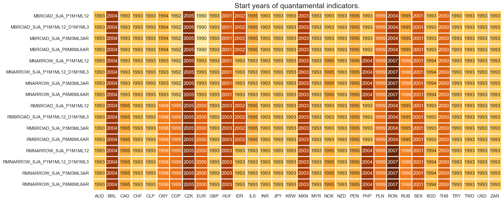
Most developed countries have both broad and narrow countries available since the 1990’s with Sweden being an exception, and for the rest of countries they are available since the early 2000’s

xcatx = main
cidx = cids_exp

dfx = msm.reduce_df(df, xcats=xcatx, cids=cidx)
dfs = msm.check_startyears(dfx)
msm.visual_paneldates(dfs, size=(18, 8))

print("Last updated:", date.today())

Last updated: 2025-07-03

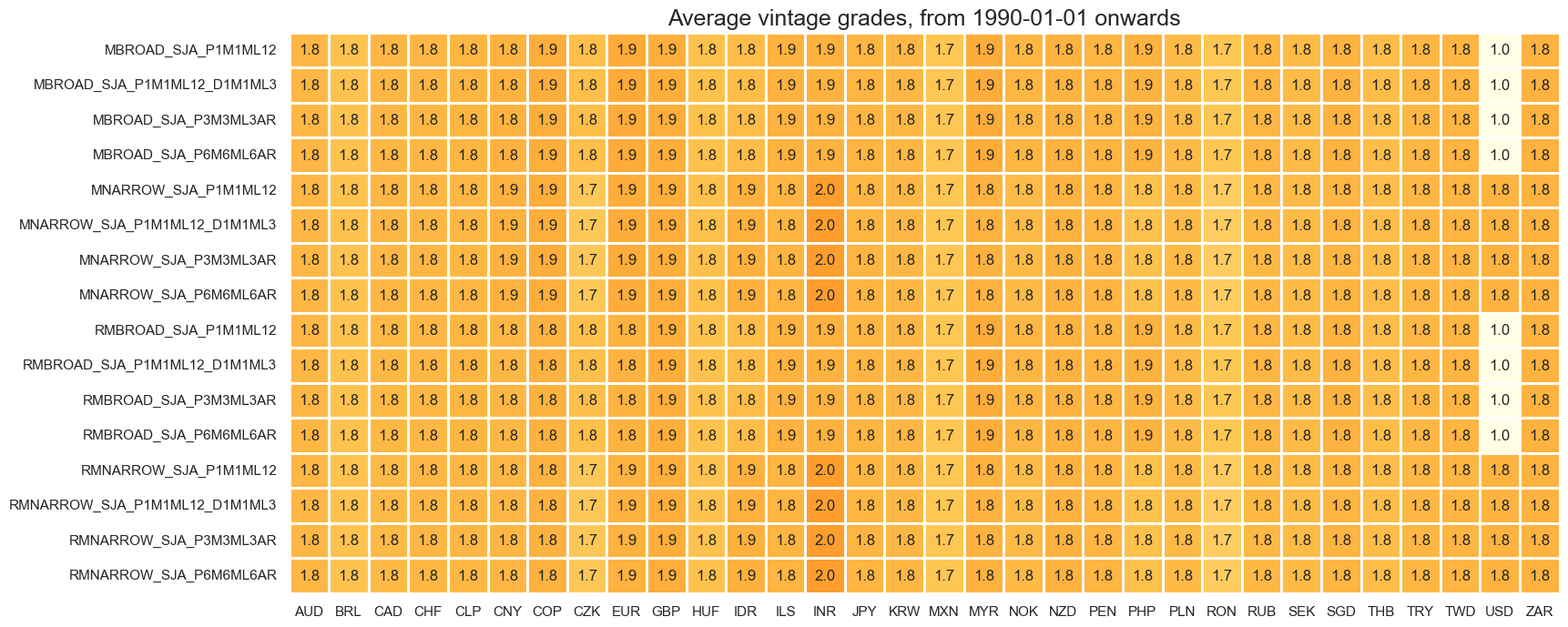
Vintage grades are fairly uniform throughout the cross sections, with a lower average due to seasonal-adjustment reflecting a good proxy of real time data.

plot = msp.heatmap_grades(
    df,
    xcats=xcatx,
    cids=cidx,
    start=start_date,
    size=(18, 8),
    title=f"Average vintage grades, from {start_date} onwards",
)

narrow = [
    "RMNARROW_SJA_P1M1ML12",
    "MNARROW_SJA_P1M1ML12",
]
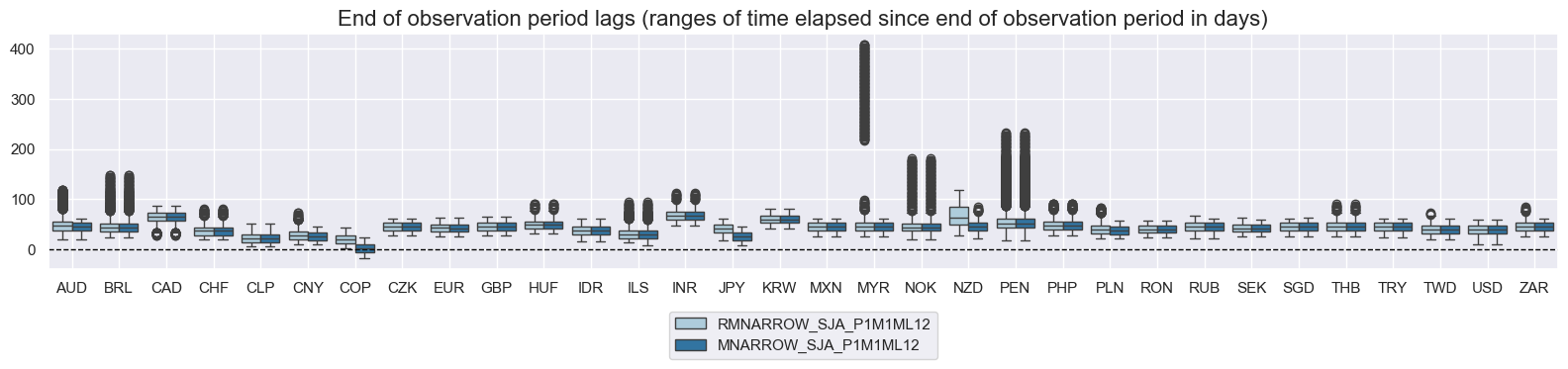
msp.view_ranges(
    df,
    xcats=narrow,
    cids=cids_exp,
    val="eop_lag",
    title="End of observation period lags (ranges of time elapsed since end of observation period in days)",
    start="2000-01-01",
    kind="box",
    size=(16, 4),
)
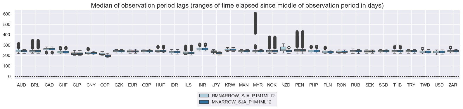
msp.view_ranges(
    df,
    xcats=narrow,
    cids=cids_exp,
    val="mop_lag",
    title="Median of observation period lags (ranges of time elapsed since middle of observation period in days)",
    start="2000-01-01",
    kind="box",
    size=(16, 4),
)

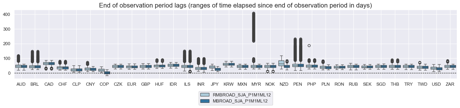
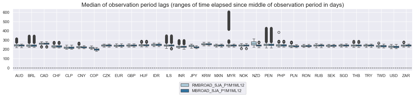
narrow = [
    "RMBROAD_SJA_P1M1ML12",
    "MBROAD_SJA_P1M1ML12",
]
msp.view_ranges(
    df,
    xcats=narrow,
    cids=cids_exp,
    val="eop_lag",
    title="End of observation period lags (ranges of time elapsed since end of observation period in days)",
    start="2000-01-01",
    kind="box",
    size=(16, 4),
)
msp.view_ranges(
    df,
    xcats=narrow,
    cids=cids_exp,
    val="mop_lag",
    title="Median of observation period lags (ranges of time elapsed since middle of observation period in days)",
    start="2000-01-01",
    kind="box",
    size=(16, 4),
)

History

Narrow money

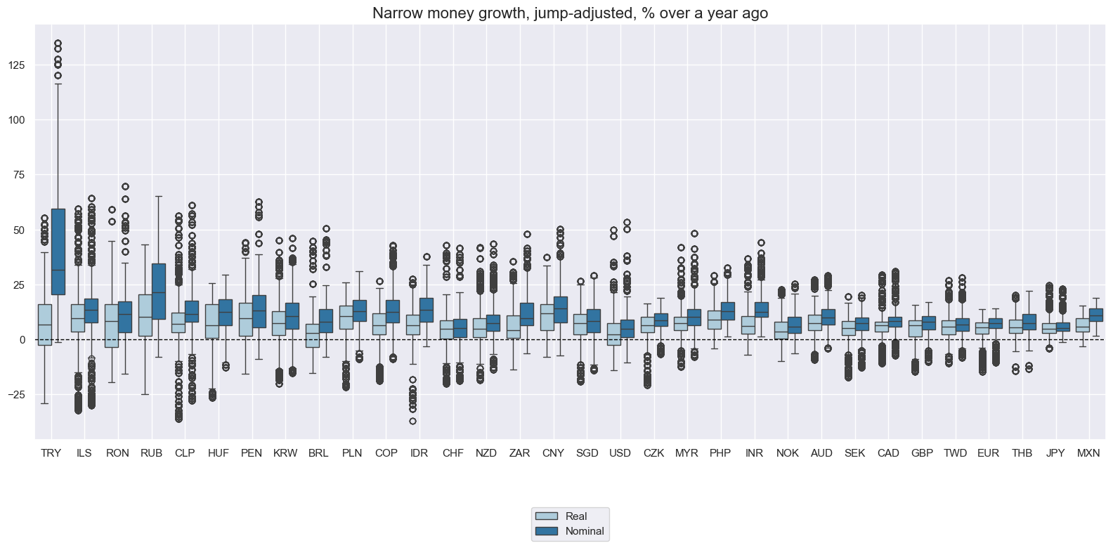
Narrow money growth rates are prone to outliers. Credible inflation-targeting countries have posted similar ranges of expansion since the 1990s.

xcatx = [
    "RMNARROW_SJA_P1M1ML12",
    "MNARROW_SJA_P1M1ML12",
]
cidx = cids_exp

msp.view_ranges(
    df,
    xcats=xcatx,
    cids=cidx,
    sort_cids_by="std",
    start=start_date,
    kind="box",
    size=(16, 8),
    title="Narrow money growth, jump-adjusted, % over a year ago",
    xcat_labels=["Real", "Nominal"],
)

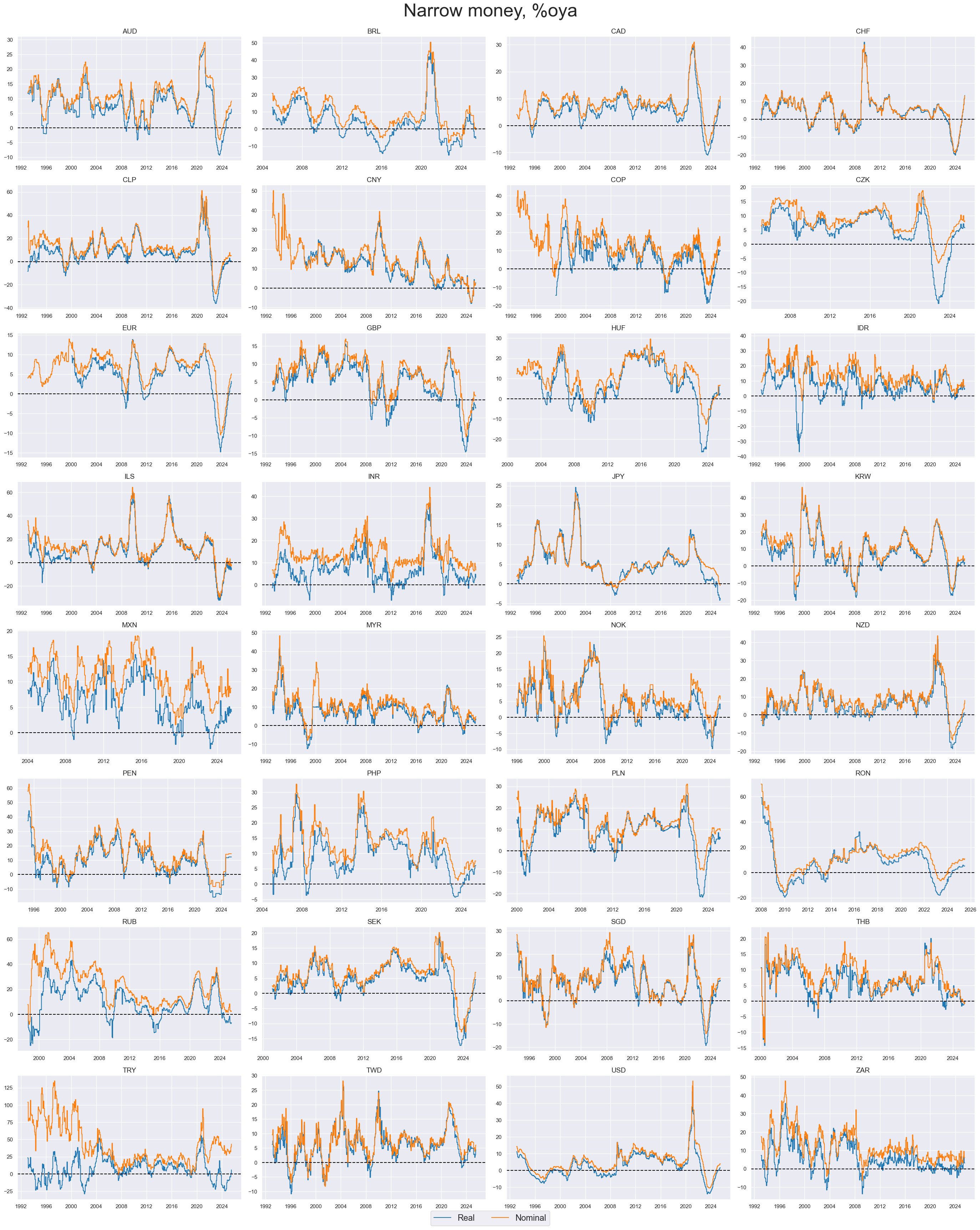
Narrow money growth has posted pronounced cycles over the past decades. Negative values are frequent occurrences.

xcatx = ["RMNARROW_SJA_P1M1ML12", "MNARROW_SJA_P1M1ML12"]
cidx = cids_exp

msp.view_timelines(
    df,
    xcats=xcatx,
    cids=cidx,
    start=start_date,
    title="Narrow money, %oya",
    xcat_labels=["Real", "Nominal"],
    title_fontsize=37,
    legend_fontsize=17,
    ncol=4,
    same_y=False,
    size=(16, 8),
    all_xticks=True,
)

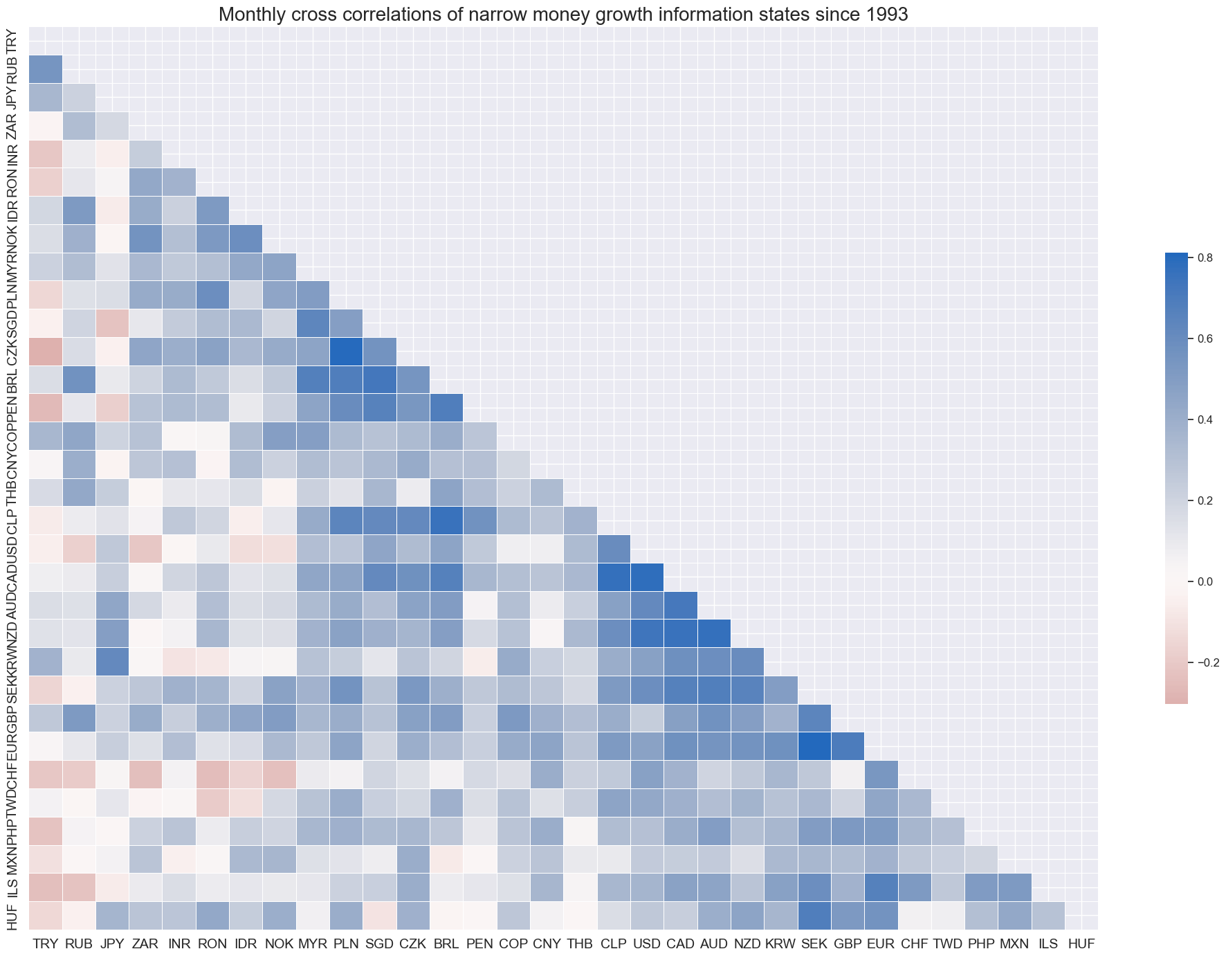
Cross-country correlation of reported narrow money growth has been mostly positive, but Japan and some EM countries have shown mostly idiosyncratic behaviour.

xcatx = ["MNARROW_SJA_P1M1ML12"]
cidx = cids_exp

msp.correl_matrix(
    df,
    xcats=xcatx,
    cids=cidx,
    size=(20, 14),
    cluster=True,
    freq="M",
    title="Monthly cross correlations of narrow money growth information states since 1993",
)

Broad money

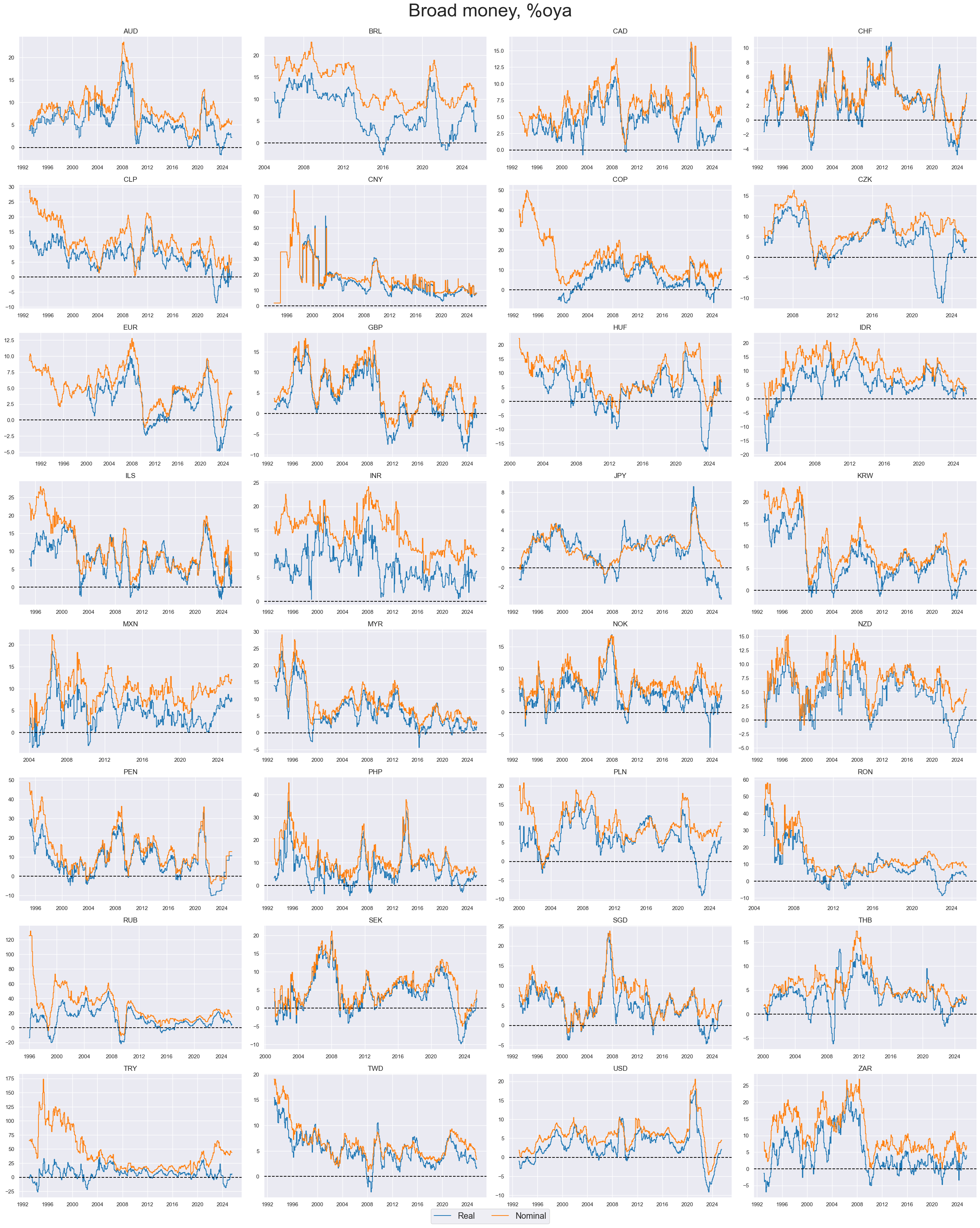
Broad money growth rates likewise show cyclical patterns but with many erratic movements.

xcatx = ["RMBROAD_SJA_P1M1ML12", "MBROAD_SJA_P1M1ML12"]
cidx = cids_exp

msp.view_timelines(
    df,
    xcats=xcatx,
    cids=cidx,
    start=start_date,
    title="Broad money, %oya",
    xcat_labels=["Real", "Nominal"],
    title_fontsize=37,
    legend_fontsize=17,
    ncol=4,
    same_y=False,
    size=(16, 8),
    all_xticks=True,
)

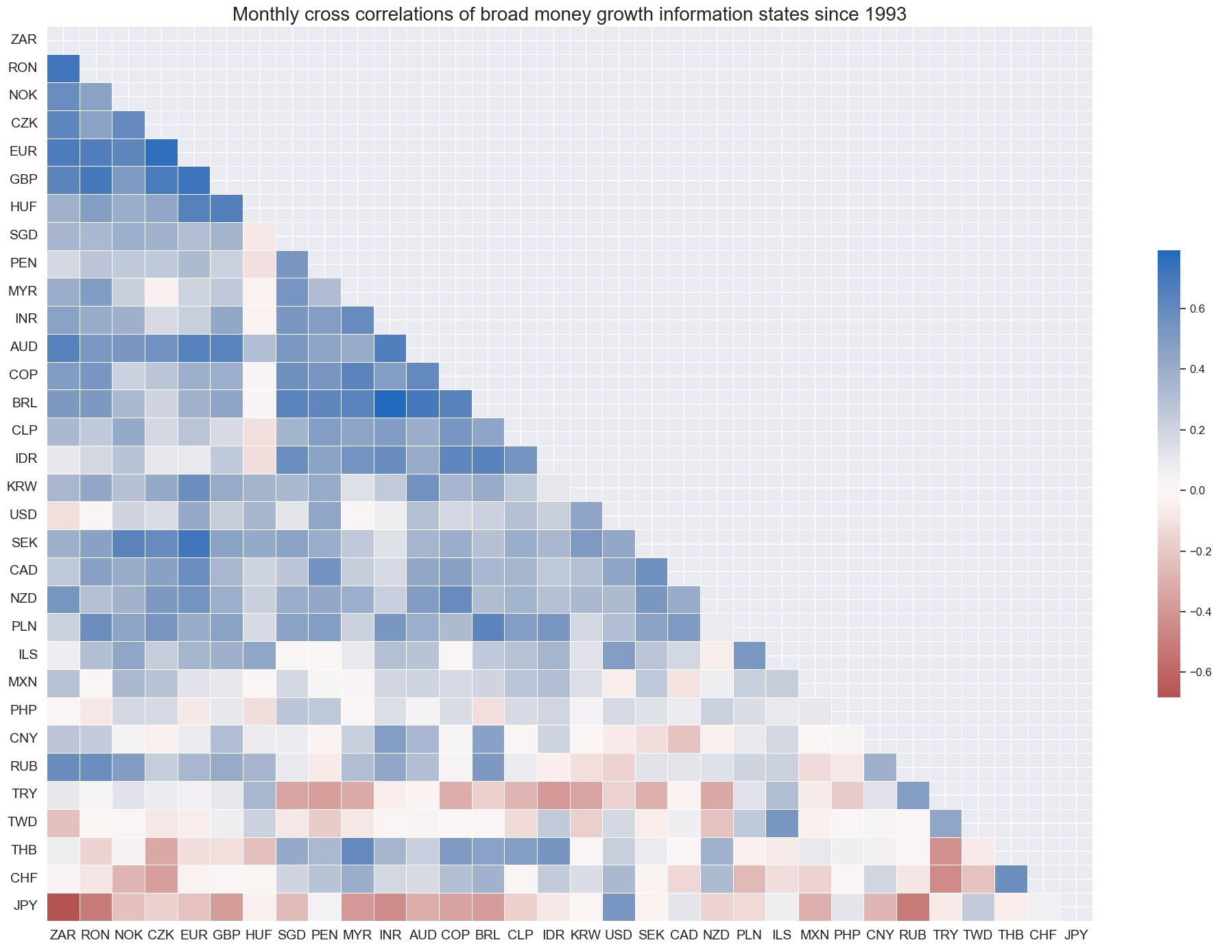
Cross-country correlation of M3 growth has been fairly diverse.

xcatx = ["MBROAD_SJA_P1M1ML12"]
cidx = cids_exp

msp.correl_matrix(
    df,
    xcats=xcatx,
    cids=cidx,
    size=(20, 14),
    cluster=True,
    freq="M",
    title="Monthly cross correlations of broad money growth information states since 1993",
)

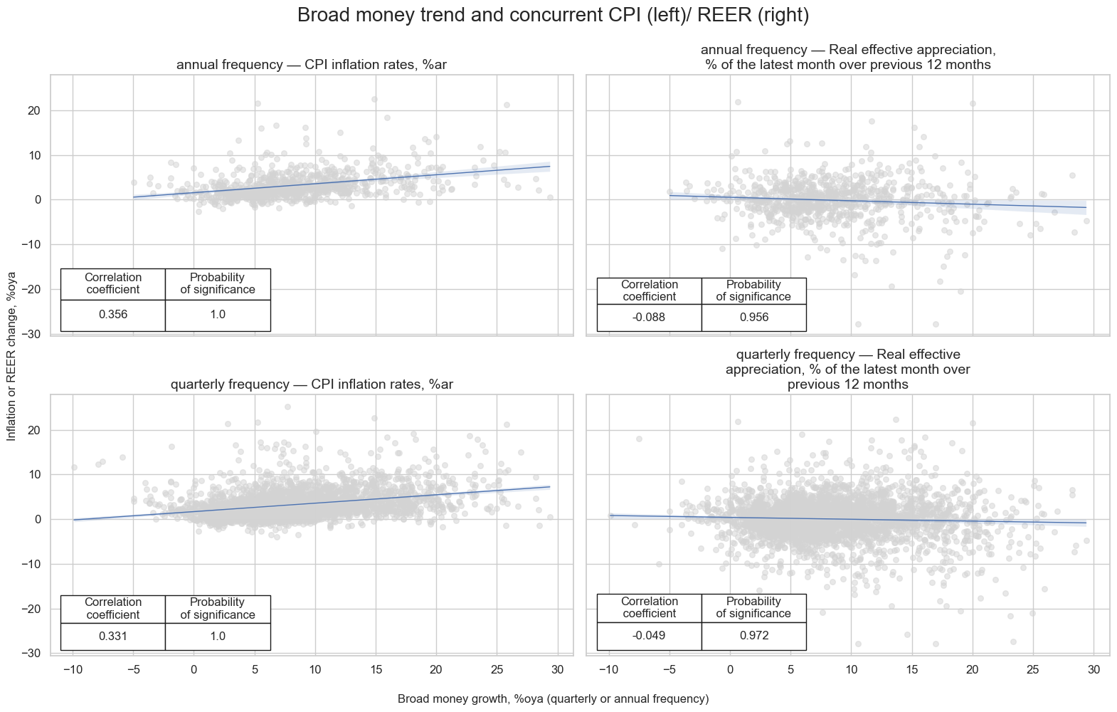
Short-term broad and narrow money growth is positively correlated with inflation because rising money supply increases demand in the economy, which can push prices higher when output doesn’t keep pace. Additionally, both money growth and inflation often rise together during economic expansions, and central banks may further boost money supply in response to inflation or growth pressures—reinforcing the correlation. Broad money growth is expected to be negatively correlated with the REER because monetary expansion tends to weaken the domestic currency through lower real interest rates, higher inflation, and reduced capital inflows, leading to a decline in the real effective exchange rate.

freqs = {
    "A": "annual frequency",
    "Q": "quarterly frequency"
}

relations = []

target_names = {
    "CPIH_SA_P1M1ML12": "CPI inflation rates, %ar",
    "REER_NSA_P1M12ML1": "Real effective appreciation, % of the latest month over previous 12 months"
}

subplot_titles = [
    f"{freqs[freq]} — {target_names[target]}"
    for freq in freqs
    for target in target_names.keys()
]


for freq in freqs:
    for target in target_names.keys():
        cr = msp.CategoryRelations(
            df,
            xcats=["MBROAD_SJA_P1M1ML12", target],
            cids=cids,
            freq=freq,
            lag=0,
            xcat_aggs=["last", "last"],
            xcat_trims=(30, 30),
            start="2000-01-01",
        )
        relations.append(cr)

msv.multiple_reg_scatter(
    cat_rels=relations,
    title="Broad money trend and concurrent CPI (left)/ REER (right)",
    xlab="Broad money growth, %oya (quarterly or annual frequency)",
    ylab="Inflation or REER change, %oya",
    ncol=2,
    nrow=2,
    figsize=(16, 10),
    prob_est="map",
    coef_box="lower left",
    subplot_titles=subplot_titles
)

Importance

Research links

“First, governments can capture real resources through base money creation (seigniorage). Seigniorage represents the real revenues a government acquires by using newly issued money to buy goods and non-money asset.” Macrosynergy

“Moreover, the moment investors anticipate inflationary financing, interest rates would rise, reducing the gains from debt monetization, up to the point of undermining its effectiveness altogether.” Macrosynergy

“Higher money growth predicts lower stock returns.” Böing & Stadtmann

“… increases in the supply of money are thought to trigger a rebalancing of the liquidity/asset ratio compatible with optimal portfolio allocation of each institution, which leads to a higher demand for assets and thus asset price increases.” Adalid & Detken

“In terms of causality, we find that monetary aggregates are frequently affected changes in stock prices, possibly mirroring portfolio adjustments in times of financial stress.” Belke, Beckmann

Empirical clues

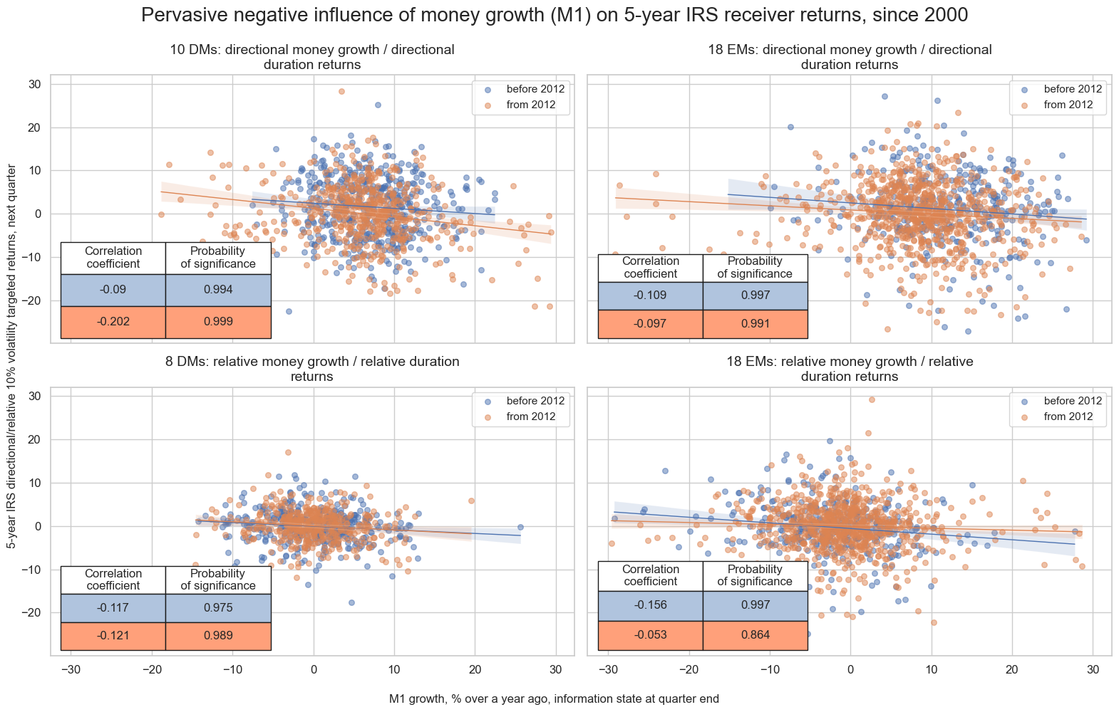
Monetary aggregates and directional/relative duration returns

Money growth is not carefully monitored by markets anymore and rarely used in systematic trading strategies. However, it plausibly is related to financial system expansion and money-driven inflation. Indeed, empirically there has been pervasive and significant predictive power of money growth for subsequent duration (5-year IRS receiver) returns over past decades. Negative forward correlation can be found for developed and emerging markets, and for both directional and relative returns. It also has been stable across sub-samples.

dfx = df.copy()

for cids, postfix in [(cids_dm, "vDM"), (cids_em, "vEM")]:
    dfa = msp.make_relative_value(
        dfx,
        xcats=main + ["DU05YXR_VT10"],
        cids=cids,
        postfix=postfix,
    )
    dfx = msm.update_df(dfx, dfa)

dfb = dfx[dfx["xcat"].isin(["FXTARGETED_NSA", "FXUNTRADABLE_NSA"])].loc[
    :, ["cid", "xcat", "real_date", "value"]
]
dfba = (
    dfb.groupby(["cid", "real_date"])
    .aggregate(value=pd.NamedAgg(column="value", aggfunc="max"))
    .reset_index()
)
dfba["xcat"] = "FXBLACK"
fxblack = msp.make_blacklist(dfba, "FXBLACK")

em_cids = list(set(msm.common_cids(dfx, xcats=["MNARROW_SJA_P1M1ML12", "DU05YXR_VT10"])).intersection(set(cids_em) - {"TRY"}))

region_configs = {
    "DM_dir": {
        "signal_pairs": [
            ("MNARROW_SJA_P1M1ML12", "DU05YXR_VT10"),
        ],
        "cids": cids_dm,
        "subplot_titles": [
            f"{len(cids_dm)} DMs: directional money growth / directional duration returns",
        ],
    },
    "EM_dir": {
        "signal_pairs": [
            ("MNARROW_SJA_P1M1ML12", "DU05YXR_VT10")
        ],
        "cids": em_cids,
        "subplot_titles": [
            f"{len(em_cids)} EMs: directional money growth / directional duration returns",
        ],
    },
    "DM_rel": {
        "signal_pairs": [
            ("MNARROW_SJA_P1M1ML12vDM", "DU05YXR_VT10vDM"),
        ],
        "cids": cids_dmfx,
        "subplot_titles": [
            f"{len(cids_dmfx)} DMs: relative money growth / relative duration returns",
        ],
    },
    "EM_rel": {
        "signal_pairs": [
            ("MNARROW_SJA_P1M1ML12vEM", "DU05YXR_VT10vEM")
        ],
        "cids": em_cids,
        "subplot_titles": [
            f"{len(em_cids)} EMs: relative money growth / relative duration returns",
        ],
    },
}

# Collect all CategoryRelations objects and subplot titles
all_relations = []
all_titles = []

for region, config in region_configs.items():
    for i, (sig, targ) in enumerate(config["signal_pairs"]):
        cr = msp.CategoryRelations(
            dfx,
            xcats=[sig, targ],
            cids=config["cids"],
            freq="Q",
            lag=1,
            blacklist=fxblack,
            xcat_aggs=["last", "sum"],
            start="2000-01-01",
            xcat_trims=(30, 30), # for plot focus
        )
        all_relations.append(cr)
        all_titles.append(config["subplot_titles"][i])

msv.multiple_reg_scatter(
    cat_rels=all_relations,
    title="Pervasive negative influence of money growth (M1) on 5-year IRS receiver returns, since 2000",
    xlab="M1 growth, % over a year ago, information state at quarter end",
    ylab="5-year IRS directional/relative 10% volatility targeted returns, next quarter",
    ncol=2,
    nrow=2,
    separator=2012,
    figsize=(16, 10),
    prob_est="map",
    coef_box="lower left",
    subplot_titles=all_titles
)

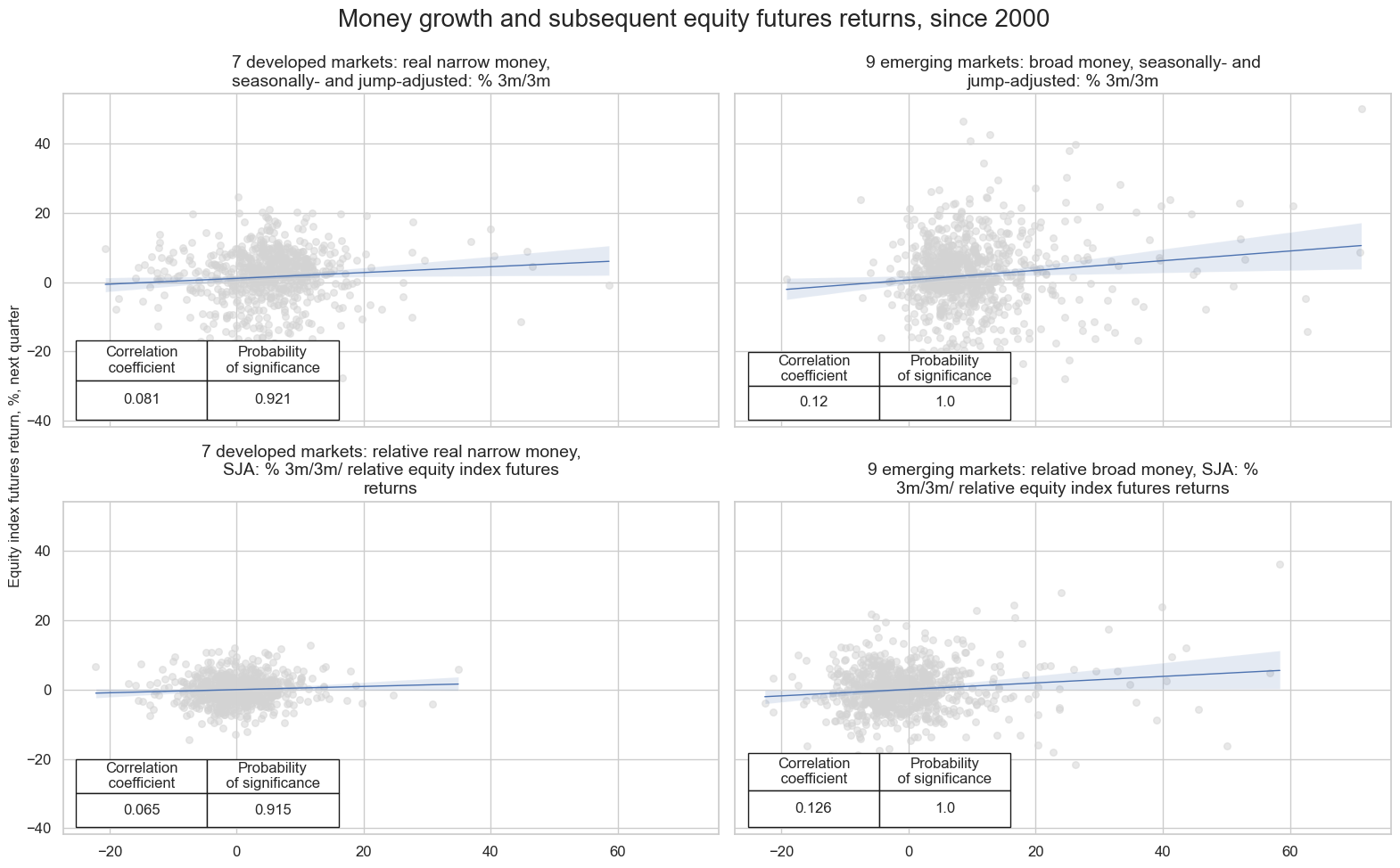
Monetary aggregates and equity returns

Contrary to duration returns, there is evidence of a significant positive relationship between short-term money growth and subsequent equity returns. This forward correlation is statistically significant at both monthly and quarterly frequencies and holds for both directional and relative return measures.

for cids, postfix in [(cids_dmeq, "vDM"), (cids_emeq, "vEM")]:
    dfa = msp.make_relative_value(
        dfx,
        xcats=main + ["EQXR_NSA", "EQXR_VT10"],
        cids=cids,
        postfix=postfix,
    )
    dfx = msm.update_df(dfx, dfa)

# Define a list of region configurations
region_configs = [
    {
        "sig": "RMNARROW_SJA_P3M3ML3AR",
        "targ": "EQXR_NSA",
        "cids": cids_dmeq,
        "title": f"{len(cids_dmeq)} developed markets: real narrow money, seasonally- and jump-adjusted: % 3m/3m "
    },
    {
        "sig": "MBROAD_SJA_P3M3ML3AR",
        "targ": "EQXR_NSA",
        "cids": cids_emeq,
        "title": f"{len(cids_emeq)} emerging markets: broad money, seasonally- and jump-adjusted: % 3m/3m "
    },
        {
        "sig": "RMNARROW_SJA_P3M3ML3ARvDM",
        "targ": "EQXR_NSAvDM",
        "cids": cids_dmeq,
        "title": f"{len(cids_dmeq)} developed markets: relative real narrow money, SJA: % 3m/3m/ relative equity index futures returns"
    },
    {
        "sig": "MBROAD_SJA_P3M3ML3ARvEM",
        "targ": "EQXR_NSAvEM",
        "cids": cids_emeq,
        "title": f"{len(cids_emeq)} emerging markets: relative broad money, SJA: % 3m/3m/ relative equity index futures returns"
    }
]

# Collect all CategoryRelations objects and subplot titles
all_relations = []
all_titles = []

for cfg in region_configs:
    cr = msp.CategoryRelations(
        dfx,
        xcats=[cfg["sig"], cfg["targ"]],
        cids=cfg["cids"],
        freq="q",
        lag=1,
        xcat_aggs=["last", "sum"],
        start="2000-01-01",
    )
    all_relations.append(cr)
    all_titles.append(cfg["title"])


msv.multiple_reg_scatter(
    cat_rels=all_relations,
    title="Money growth and subsequent equity futures returns, since 2000",
    xlab="",
    ylab="Equity index futures return, %, next quarter",
    ncol=2,
    nrow=2,
    figsize=(16, 10),
    prob_est="map",
    coef_box="lower left",
    subplot_titles=all_titles
)

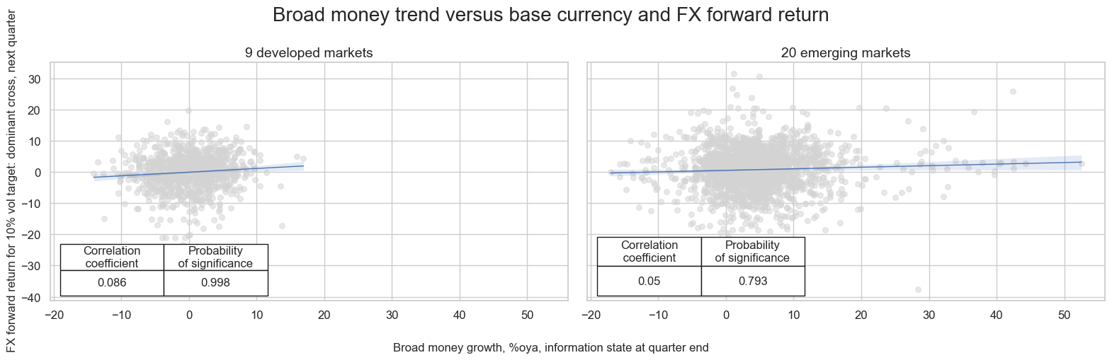
Monetary aggregates and FX returns

Empirical evidence suggests that relative broad money growth positively predicts FX forward returns. The relation has been significant and a monthly and quarterly frequency and for both developed markets and EM currencies. Strong broad money growth typically reflects financial expansion and conditions tighter monetary policy.

xcatx = ["MBROAD_SJA_P1M1ML12"]

for xc in xcatx:
    calc_eur = [f"{xc}vBM = {xc} - iEUR_{xc}"]
    calc_usd = [f"{xc}vBM = {xc} - iUSD_{xc}"]
    calc_eud = [f"{xc}vBM = {xc} - 0.5 * ( iEUR_{xc} + iUSD_{xc} )"]

    dfa_eur = msp.panel_calculator(dfx, calcs=calc_eur, cids=cids_eur)
    dfa_usd = msp.panel_calculator(dfx, calcs=calc_usd, cids=cids_usd + ["EUR"])
    dfa_eud = msp.panel_calculator(dfx, calcs=calc_eud, cids=cids_eud)

    dfa = msm.update_df(dfa, pd.concat([dfa_eur, dfa_usd, dfa_eud]))

dfx = msm.update_df(dfx, dfa)

region_configs = {
    "DM": {
        "signal_pairs": [
            ("MBROAD_SJA_P1M1ML12vBM", "FXXR_VT10"),
        ],
        "cids": cids_dmfx + ["EUR"],
        "subplot_titles": [
            f"{len(cids_dmfx) + 1} developed markets",
        ],
    },
    "EM": {
        "signal_pairs": [
            ("MBROAD_SJA_P1M1ML12vBM", "FXXR_VT10")
        ],
        "cids": cids_emfx,
        "subplot_titles": [
            f"{len(cids_emfx)} emerging markets",
        ],
    },
}

# Collect all CategoryRelations objects and subplot titles
all_relations = []
all_titles = []

for region, config in region_configs.items():
    for i, (sig, targ) in enumerate(config["signal_pairs"]):
        cr = msp.CategoryRelations(
            dfx,
            xcats=[sig, targ],
            cids=config["cids"],
            freq="q",
            lag=1,
            blacklist=fxblack,
            xcat_aggs=["last", "sum"],
            start="2000-01-01",
        )
        all_relations.append(cr)
        all_titles.append(config["subplot_titles"][i])


msv.multiple_reg_scatter(
    cat_rels=all_relations,
    title="Broad money trend versus base currency and FX forward return",
    xlab="Broad money growth, %oya, information state at quarter end",
    ylab="FX forward return for 10% vol target: dominant cross, next quarter",
    ncol=2,
    nrow=1,
    figsize=(16, 5),
    prob_est="map",
    coef_box="lower left",
    subplot_titles=all_titles
)

Appendices

Appendix 1: Currency symbols

The word ‘cross-section’ refers to currencies, currency areas or economic areas. In alphabetical order, these are AUD (Australian dollar), BRL (Brazilian real), CAD (Canadian dollar), CHF (Swiss franc), CLP (Chilean peso), CNY (Chinese yuan renminbi), COP (Colombian peso), CZK (Czech Republic koruna), DEM (German mark), ESP (Spanish peseta), EUR (Euro), FRF (French franc), GBP (British pound), HKD (Hong Kong dollar), HUF (Hungarian forint), IDR (Indonesian rupiah), ITL (Italian lira), JPY (Japanese yen), KRW (Korean won), MXN (Mexican peso), MYR (Malaysian ringgit), NLG (Dutch guilder), NOK (Norwegian krone), NZD (New Zealand dollar), PEN (Peruvian sol), PHP (Philippine peso), PLN (Polish zloty), RON (Romanian leu), RUB (Russian ruble), SEK (Swedish krona), SGD (Singaporean dollar), THB (Thai baht), TRY (Turkish lira), TWD (Taiwanese dollar), USD (U.S. dollar), ZAR (South African rand).