Macro trading factors: dimension reduction and statistical learning

Jupyter Notebook

Macro trading factors are information states of economic developments that help predict asset returns. A single factor is typically represented by multiple indicators, just as a trading signal often combines several factors. Like signal generation, factor construction can be supported by regression-based statistical learning. Dimension reduction is particularly useful for factor discovery. It is the transformation of high-dimensional data into a lower-dimensional representation that retains most of the information content. Dimension reduction methods, such as principal components and partial least squares, reduce bias, increase objectivity, and strengthen the reliability of backtests.

This post applies statistical learning with dimension-reduction techniques to macro factor generation for developed fixed-income markets. The method adapts to the degree of theoretical guidance and the complexity of the data. Several dimension-reduction approaches have successfully produced factors for interest-rate swap trading, delivering positive predictive power, strong accuracy, and robust long-term PnL.

The post below is based on Macrosynergy’s proprietary research. Please quote as “Gholkar, Rushil and Sueppel, Ralph, ‘Macro trading factors: dimension reduction and statistical learning,’ Macrosynergy research post, September 2025.” This post extends and supersedes a previous article, “Using principal components to construct macro trading signals.”

A Jupyter notebook for auditing and replicating the research results can be downloaded here. The notebook operation requires access to J.P. Morgan DataQuery to download data from JPMaQS. Everyone with DataQuery access can download data except for the latest months. Moreover, J.P. Morgan offers free trials on the complete dataset for institutional clients. An academic support program sponsors data sets for research projects.

Macro trading factor generation: high-level perspective

A macro trading factor is a time series or panel (time series across multiple markets) of point-in-time information that is presumed to predict subsequent financial returns. Here, the focus is on macro-quantamental factors, which represent actual macroeconomic information, rather than just market prices and flows. Such factors are typically calculated using one or more underlying macro-quantamental indicators, i.e., point-in-time information states of economic concepts that are monitored by financial markets and are available in real-time from the J.P. Morgan Macrosynergy Quantamental System (JPMaQS).

A macro trading factor is not yet a trading signal. Signals govern risk and positioning in specific markets over time, consider desirable features of the portfolio, and are often based on multiple factors. Indeed, the construction of trading signals from multiple factors is a major field of machine learning methods, which can detect patterns unsuspected by human strategy developers and produce high-quality backtests without hindsight biases.

Just as machine learning supports the construction of trading signals from trading factors, so can it also help build trading factors from underlying indicator time series. However, objectives and methods are slightly different:

• In signal generation, we combine multiple valid trading factors such that we have reason to expect that the composite delivers consistently profitable trades. Thus, we optimize predictive power, directional accuracy, and steadfastness of value generation. Conceptual and statistical diversity are desirable.
• In factor generation, we combine multiple indicators or categories (i.e., similar indicators across countries) to extract their primary common type of information. One conceptual factor is often represented by numerous time series. For example, the concept “inflation” is captured by multiple growth rates and multiple price indices. Thus, we optimize the retention of original information while reducing the complexity of available data. Conceptual and statistical diversity of the original indicators is undesirable. If indicators have little conceptual overlap, for example, they should be categorized into different factors.

The formation of a conceptual factor is principally a matter of theory and convention. For example, the concept “inflation” refers to changes in the money price of goods and services, and only a certain type of economic indicator can represent it. Even if, on occasion, a production indicator is highly correlated with inflation, it does not belong to that group. Moreover, central banks and markets typically focus on a subset of available inflation indicators, and that subset would shape the bulk of perceptions. Against that backdrop, it is a legitimate approach to represent conceptual factors by weighted or unweighted averages of conventionally monitored indicators. This approach is often taken in Macrosynergy posts. However, statistical methods of dimension reduction, such as principal components analysis and partial least squares, can still add considerable benefits.

• Bias reduction: There is usually no clear guidance for setting the weights of different categories that could represent a conceptual factor. Parity across sub-concepts is a popular option, but a very rough one that disregards how important and representative an indicator really is.
• Objectivity: The choice and weight of data categories in conceptual factors may be colored by hindsight. By contrast, sequential statistical extraction, based solely on data up to the extracted factor’s point in time, is an objective method more conducive to reliable backtests.

Regression-based learning with dimension reduction

We propose regression-based statistical learning with factors that have been calculated based on dimension reduction. Regression-based learning can optimize model parameters and hyperparameters sequentially and produce signals based on whatever model has predicted returns best up to a point in time. This has been explained in previous posts (Macro trading signal optimization: basic statistical learning methods and Regression-based macro trading signals). The purpose of dimension reduction is to convert a high-dimensional data set into a lower-dimensional one while keeping most of the original information. It makes regressors simpler, easier to interpret, and less noisy. In this post, we look at two methods that combine regression and dimension reduction:

• Principal components regression (PCR) is a linear regression technique that uses principal components as regressors. It addresses the problems arising from collinearity by combining explanatory variables into a smaller set of uncorrelated variables. Collinearity is problematic for regression because it creates instability and unreliability in the model’s parameter estimates. The main benefit of using principal components is a reduction in the standard errors of regression coefficients. Simply put, we discard some information to maintain relationship stability. Principal components are combinations of the original variables, whose squared weights add up to 1, and which are extracted from the eigenvectors of the covariance matrix. An eigenvector of a covariance matrix represents a direction of maximum variance in the data. Principal components are presented as centered scores.
  A shortfall of the method, however, is that it combines regressors without consideration of the dependent variable of a project. This means that principal components regression may give high weights to explanatory variables that have little explanatory power, merely based on their ability to capture a large part of the variation in the explanatory data. See more notes on principal components calculation in the present context in Annex 1.
• Partial least squares regression (PLS) is a statistical method that combines features of principal component analysis and multiple regression. The core idea behind PLS is to extract latent factors from the predictor variables that best explain the variance in both the predictors and the response variables simultaneously. PLS seeks components that maximize the covariance between the X and Y variable sets. That is why the method is also called “projection to latent structures”.
  Similar to PCR, the squared coefficients that combine original variables to a latent variable must sum to one. There is a relation between these coefficients and the covariance of the resultant latent variable with the explanatory variable. PLS coefficients for the first latent variable are found by optimizing the covariance of the latent variable with the explanatory variable. This latent variable is then used by means of ordinary least squares to explain the target variable. If one multiplies the OLS coefficients by the latent variable coefficients, one gets the final coefficients of the original variables. This is why it is called “partial” least squares: only part of the coefficient is estimated through least squares. PLS can be considered as a special way to conduct multivariate regression. In the face of high multicollinearity, confidence intervals around the PLS coefficients are usually smaller than for multivariate OLS coefficients. Hence, PLS is particularly valuable when dealing with multicollinearity among predictor variables and high-dimensional data. See more notes on principal components calculation in the present context in Annex 2.

Here, we use the term “component” generically to refer to both regular principal components (PCR) and latent variables (PLS). It is essential to carefully interpret the components of macroeconomic information states as opposed to the components of regular macroeconomic variables. Technically, a principal component is a linear combination of a set of variables that captures the maximum variance or predictive covariance in the dataset. In standard econometrics, it is often interpreted as a latent factor that drives most of the variation in the series. For example, the latent state of the business cycle may explain most of the variation in activity growth rates.

By contrast, information states often refer to different observation periods, due to varying frequencies of reported periods and different publication lags. What they do have in common on any given day is their influence on market perceptions. Hence, the main component in multiple types of information, which is the dominant pattern in various types of information, can be interpreted as the dominant force of perceptions under full information efficiency. Its predictive power arises from rational inattention, sluggish information dissemination, and delays between information and portfolio rebalancing.

Application of factor generation to global duration signals

We present a fairly simple example for the factor generation with dimension reduction. It employs regression-based statistical learning with dimension reduction to generate trading signals for duration exposure in developed markets. The signals would manage duration risk over time and across currency areas through 5-year interest rate swaps, allowing both long (fixed-rate receiver) and short (fixed-rate payer) positions to be held. The currencies we consider are AUD (Australian dollar), CAD (Canadian dollar), CHF (Swiss franc), EUR (Euro), GBP (British pound), JPY (Japanese yen), NOK (Norwegian krone), NZD (New Zealand dollar), SEK (Swedish krona), and USD (U.S. dollar).

The trading signals are based on three conceptual macro factors, all with theoretically positive effects on duration returns: inflation shortfalls, economic activity shortfalls, and money and credit growth shortfalls. To represent these factors, we consider point-in-time information states of commonly watched indicators that are available across all currency areas. These are also called quantamental categories. Quantamental categories can be downloaded from the J.P. Morgan Macrosynergy Quantamental System (JPMaQS).

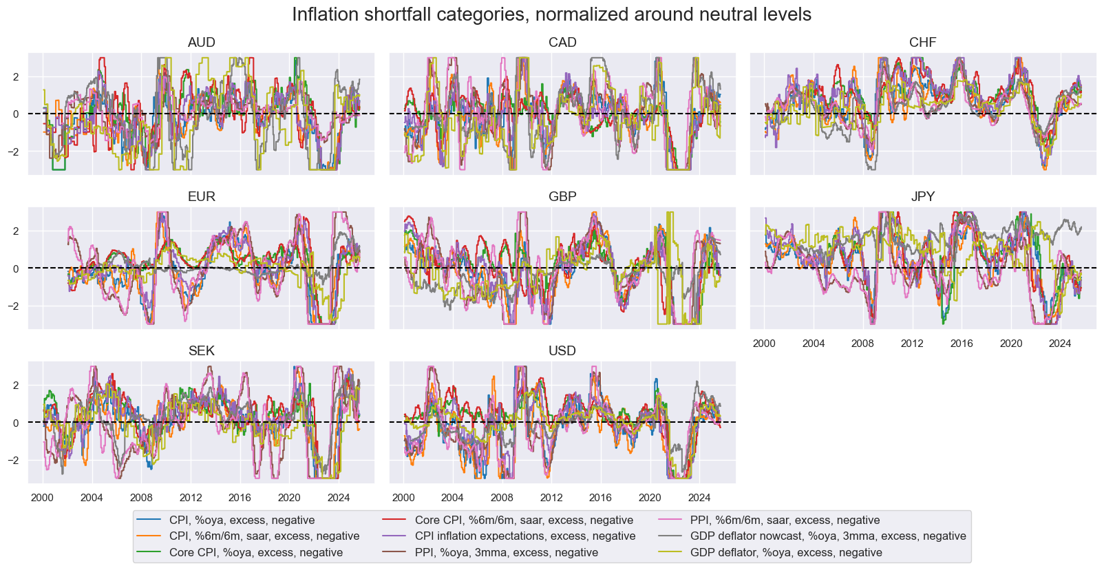
The broad inflation shortfall factor is represented by categories that indicate negative excess price pressure in the economy. It can be divided into two narrow factors: consumer price index (CPI) inflation shortfalls and producer price inflation shortfalls. The exact quantamental categories used for these two narrow factor groups are summarized in Annex 3, and their normalized dynamics are plotted below. Here, normalization means sequential adjustment of category values around their theoretical neutral levels, based on panel data concurrently available. Generally, excess inflation is calculated vis-à-vis the effective inflation target, which is a combination of the official target and past performance versus that target (view documentation). Since 2000, all inflation shortfall metrics have followed similar broad patterns but with differences in size and timing of fluctuations.

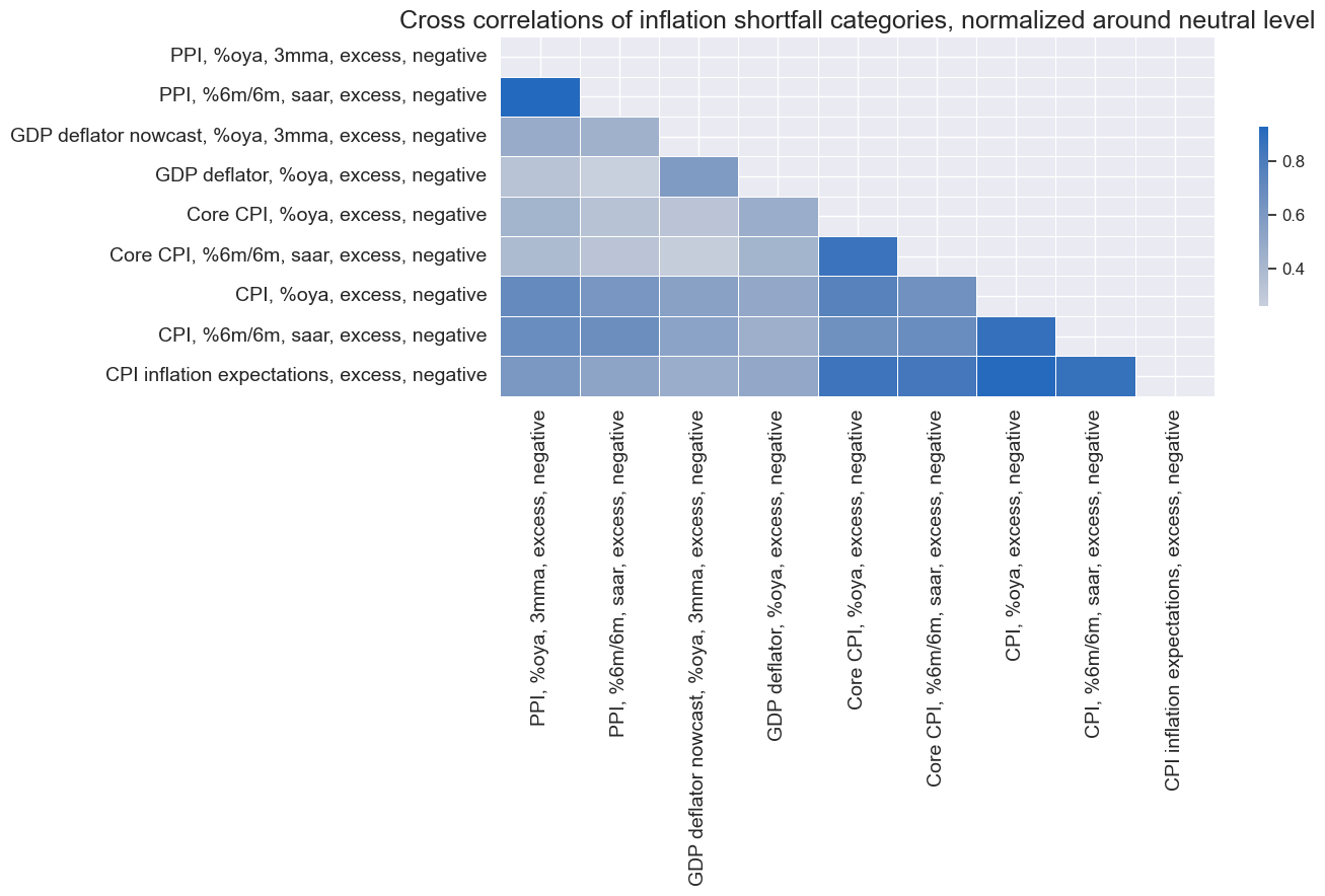
The monthly average cross-correlation of inflation shortfall categories since 2000, for the whole panel, shows that all have been positively correlated. The strongest correlations are evident within the CPI and PPI groups.

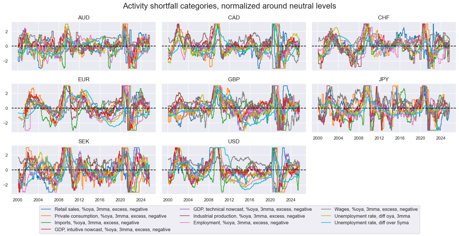
The broad activity growth shortfall factor is represented by indicators of the underperformance of spending and production growth. It consists of three narrow factors: domestic demand growth shortfalls, domestic output growth shortfalls, and labor market slack. The exact quantamental categories used for these are summarized in Annex 3, and plotted below. Generally, excess demand and output are calculated relative to 5-year trailing median GDP growth rates (view documentation). The benchmark for employment growth is workforce growth  (view documentation), and the reference for wage growth is the sum of the effective inflation target and medium-term productivity growth. While most activity shortfall indicators post similar cyclical patterns, some stand apart, particularly those related to labor market slack.

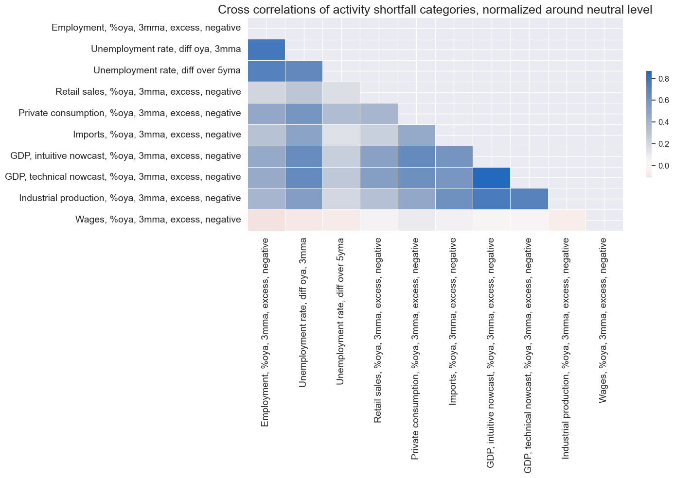
The cross-correlation of activity categories across the panel since 2000 has mostly been negative, with the notable exception of excess wage growth. Indeed, wage growth is published with longer lags in many countries and is only indirectly related to economic activity (albeit it is a legitimate indicator of labor market tightness).

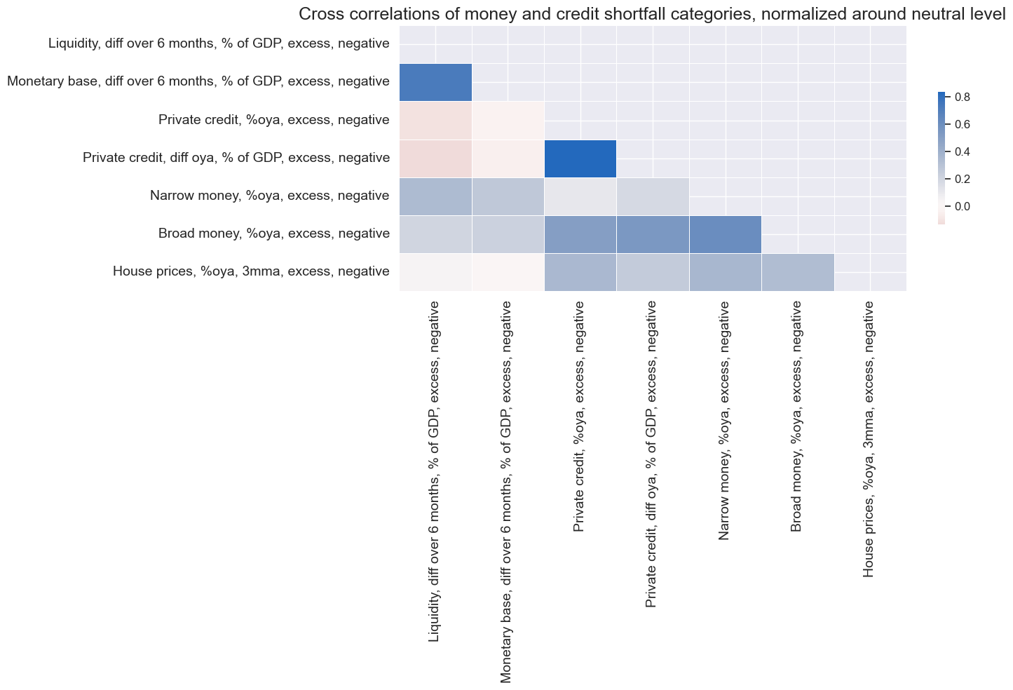
The broad money and credit growth shortfall factor is represented by indicators of slow or negative growth in private credit, monetary aggregates, or central bank liquidity. It consists of two narrow factors: credit growth shortfall and money growth shortfall. The exact quantamental categories used for the two subgroups are summarized in Annex 3, and their normalized evolution is plotted below. The dynamics of money and credit indicators are far more diverse than those of the other subgroups. Monetary base and central bank liquidity growth in particular exhibit post-idiosyncratic dynamics with large sporadic variation, mainly because they are shaped by central bank actions rather than broad economic developments.

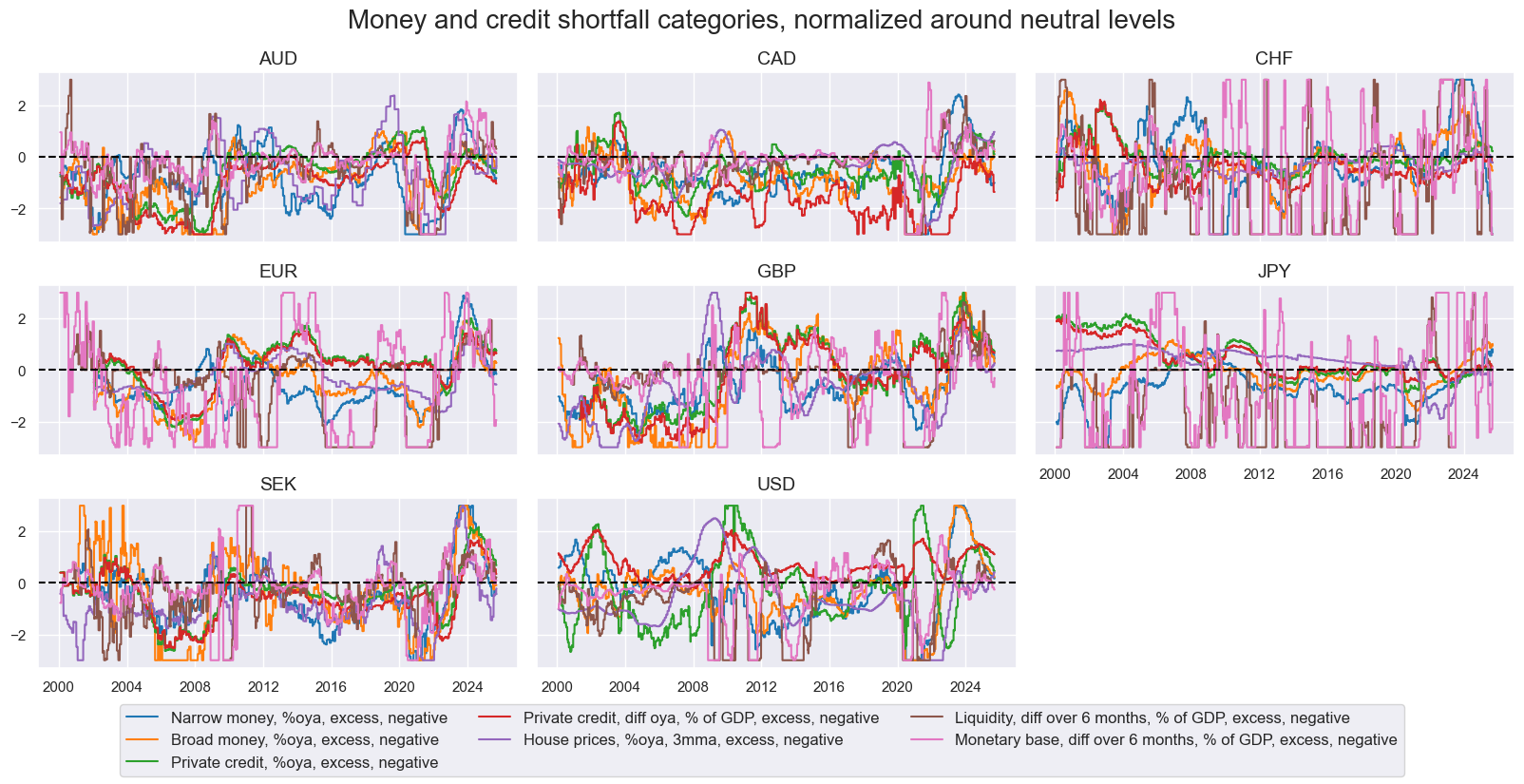
Cross-correlations of money and credit growth indicators have not been uniformly positive since 2000. Central bank liquidity expansion is typically monitored in shorter horizons and has been positively correlated with broad money growth and negatively correlated with private credit growth. The latter likely reflects that central banks’ quantitative easing is more likely in times of soft credit supply.

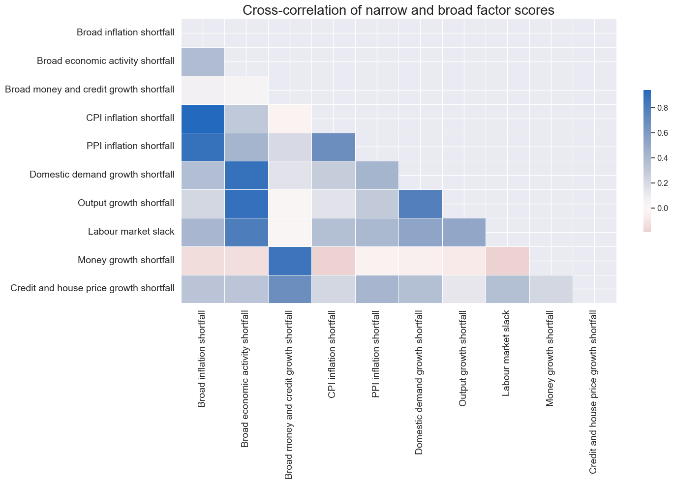
We can assess the correlation structure across both broad and narrow factor groups by calculating the averages of the normalized categories within these groups. The average correlation coefficients for the panel and since 2000 are shown below. Inflation and activity shortfalls have been modestly positively correlated, but neither has displayed much correlation with money and credit growth shortfall. Across narrow factor groups, correlation has been mostly positive, but has been above 50% only between CPI and PPI inflation and between domestic demand and output growth.

Practical guidance on different types of factor generation

In practice, sequential statistical learning with dimension reduction can support factor generation to varying degrees. The influence of dimension reduction depends inversely on the strength of the prior structure we impose. In the data example above, we defined a set of conceptual factors and assigned each factor a group of quantamental categories that could represent it. Dimension reduction can then be applied either to the full original dataset or to structured subsets to identify the three factors. Here, we consider three methods:

• The kitchen sink approach uses PCR or PLS to extract from all indicators three latent underlying variables or as many as required to explain 95% of the variation. It does not impose any theoretical factor structure. The components are then regressed onto future returns to obtain coefficients for signal generation.
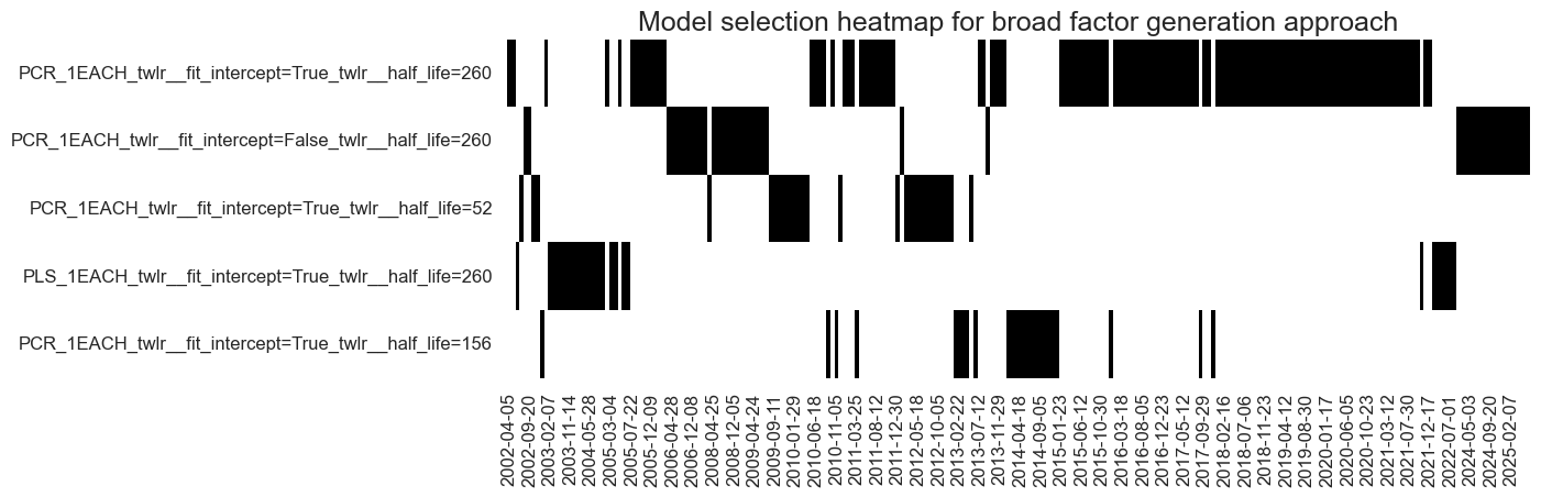
• The broad factor generation approach first applies PCR or PLS to the constituent indicators of each broad factor group and then uses the first component to represent the (broad) conceptual factor. It does not impose any structure within the broad factor group. The generated factors are then regressed on future returns to obtain coefficients for signal generation.
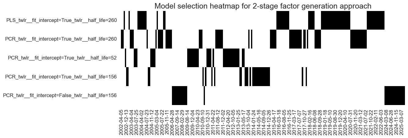
• The two-stage factor generation approach first applies PCR or PLS to the constituent indicators of each narrow factor group and uses the first principal component to represent the narrow factor. Then it applies PCR or PLS to the narrow factors under each broad factor to extract the broad factors of the second-level principal component. Then the generated broad factors are again regressed on the target returns to obtain coefficients for signal calculation.

We shall compare these methods also to a method based on theoretical priors alone. It is called two-stage conceptual parity and simply averages normalized quantamental categories within the broad factor growth and then averages the normalized factors as well. No dimension reduction or regression is required. It is thus based solely on theoretical priors. The more structure or theoretical priors we impose, the greater the bias of our learning process, i.e., the error introduced by making simplifying assumptions based on our prior beliefs. On the positive side, increased theoretical structure also reduces variance, i.e., the errors caused by model sensitivity to fluctuations in the training data.

Thus, the choice of factor generation approach, from kitchen sink to two-stage conceptual parity, is part of the bias-variance management of machine learning. Roughly speaking, a kitchen sink approach is preferable when we have ample data but lack theoretical guidance or conventions. A more structured factor generation approach is better suited when data are scarce but theory is compelling and conventions are clear.

In practice, we apply all three types of dimension reduction to sequential machine learning signal generation in three steps:

1. We define models and hyperparameters that could explain the relation between factors and target returns. Model here means principal component regression or partial least squares regression. The dimension reduction part is any of the three methods listed above, and the learning process gets to choose between principal component regression and partial least squares regression, and a few specifications. For the regression part, we offer to the learning process various time-weighted least-squares models (TWLS). Time-weighted least squares gives recent observations higher weights, often by imposing exponential time decay with a specific half-life. Key hyperparameters of the machine learning process are the inclusion or omission of a constant (given that our factors are conceptually deviations from neutral values) and the length of the half-life (which we selected here from a reasonable range of between 1, 3 and 5 years).
2. We establish the rules for cross-validation. This is the assessment of how well different models perform in predicting unseen data by dividing the available panel data set at each point in time (development data set) into multiple folds of training and test sets. This needs to respect the panel structure of our data, i.e., the presence of multiple time series across currency areas. Here, we choose the RollingKFoldPanelSplit class of the Macrosynergy package to create the folds. The training set and test set must be placed side by side in time. But the test sets can be both after and before training data. This means the method can use the past to validate a model built on future data ( see also a general introduction to panel splitters). As an evaluation criterion, we chose the standard root mean squared error.
3. Perform the actual sequential optimization with the Macrosynergy package’s specialized Python class (SignalOptimizer). It applies scikit-learn cross-validation to the specific format of macro-quantamental panel data. Here, it uses data from 2000 to start selecting optimal models and calculating optimized factors and signals on a weekly basis from 2002.

See further details on the employed Python classes in Annex 4 and the linked Jupyter notebook.

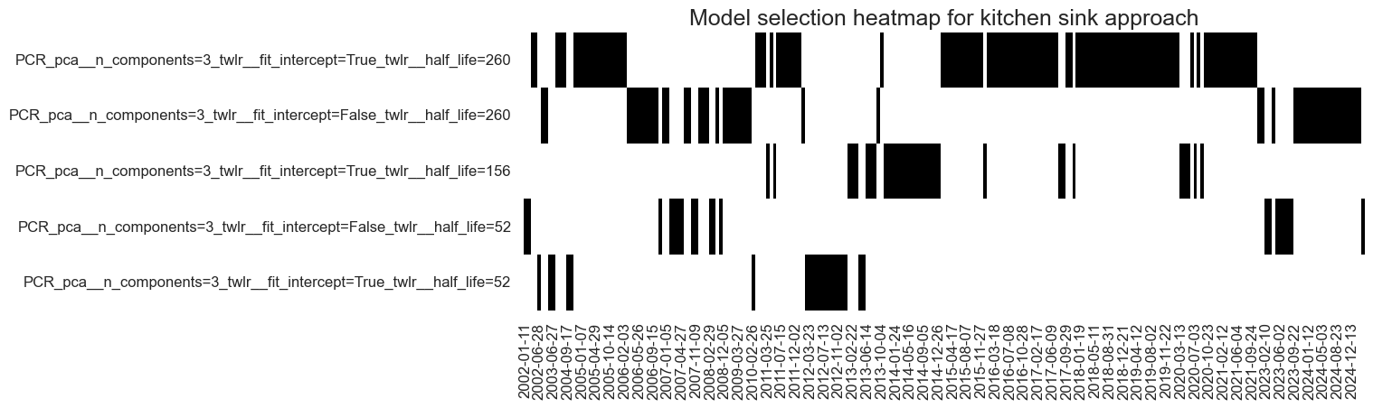
Learning with the kitchen sink approach has mostly preferred principal components regression and allowed frequent model changes until the mid-2010s. In the past two years, PCR with long (260 weeks or 5 years) and short (104 weeks or 2 years) half-life competed for the place as the best cross-validated model. There has not yet been a clear convergence on a single model. The switching between models illustrates a drawback of the learning method versus conceptual parity: changes in hyperparameters add signal variation that is unrelated to economic and market conditions.

The broad factor generation approach also mostly selected principal components regressions and failed to convincingly converge on a single model version. However, in the past 10 years, the preferred half-life of time-weighted least squares has settled on 4 years.

Finally, the two-stage factor generation approach mostly used principal components regression, but in recent years has also selected partial least squares. The preferred half-life of the exponential day of historical weights has been 3-4 years.

Empirical findings

To assess the success of factor generation with dimension reduction in our duration trading example, we look at predictive regressions, predictive accuracy measures, and backtested naive PnLs.

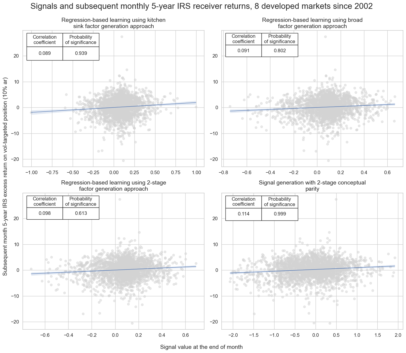
The regression scatter plots below illustrate the relationship between end-of-month signals, generated by the three learning approaches and two-stage conceptual parity, and subsequent volatility-targeted duration returns for the panel of eight developed markets since 2002. All predictive relations have been positive with roughly similar correlation coefficients of around 10%. However, only the kitchen-sink and conceptual parity approaches showed clear significance, i.e., probability of non-accidental correlation of over 90% according to the Macrosynergy panel test. It is not unusual for conceptual parity to outperform machine learning-generated signals in terms of linear correlation. This reflects partly that the learning signal features much variation due to model change, which has no predictive power.

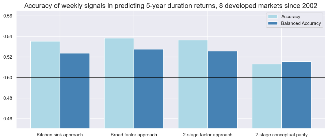
The weekly accuracy (ratio of correctly predicted weekly return signs) and balanced accuracy (average ratio of correctly predicted negative and positive returns) of all signal types have been well above 50%. In terms of accuracy, the learning signals clearly beat the conceptual parity. The difference is particularly striking for general accuracy, which is 53-54% for signals generated by machine learning with dimension reduction and just above 51% for two-stage conceptual parity. This partly reflects that the learning signal had a stronger long bias, with over 70% positive signals versus less than 50% for conceptual parity. However, the learning-based signals also posted higher balanced accuracy and beat the conceptual parity in both negative and positive precision.

We calculate naïve PnLs according to standard rules of Macrosynergy posts. End-of-week normalized signals from the learning process determine positions for the start of the next week, with a one-day slippage for execution. Signal size is capped at two standard deviations as basic risk control. The PnLs ignore transaction costs and compounding, and are scaled to a 10% annualized volatility for easier risk-adjusted return comparison across types of signals.

All signal types have generated positive long-term returns, with variations in performance statistics, seasonality, and benchmark correlations. The 23-year Sharpe ratios of the learning-based signals have been 0.6-0.7, compared to 0.6 for the conceptual parity signal. The Sortino ratios have been 0.9-1.0 for learning and 0.8-0.9 for conceptual parity. The conceptual parity PnL has been a lot more concentrated on specific periods (seasonal), particularly the early 2020s. However, learning signals have displayed a 35-40% positive correlation with the U.S. Treasury, while the conceptual parity signal has posted a slightly negative correlation.

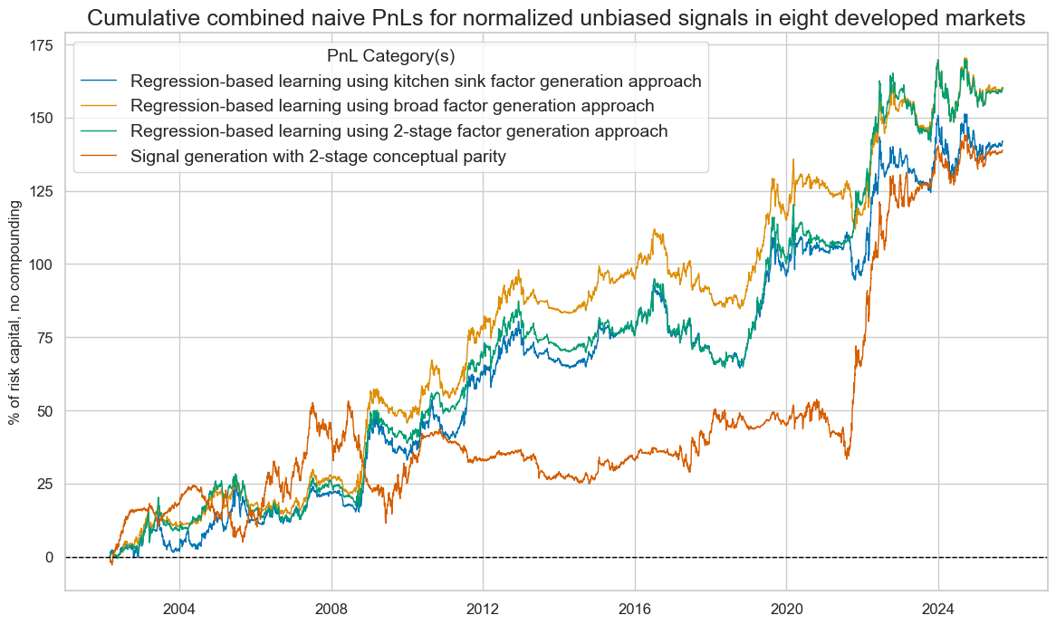
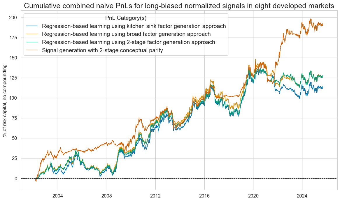
Although learning signals posted a higher risk-adjusted value in general, they did so largely by detecting positive and negative return trends and, probably, risk premia. The conceptual parity signal proved more rigid, focusing on the narrow economic hypotheses. However, when combined with a long bias, the two-stage conceptual parity signal outperformed, as most of the 2002-2025 period saw positive duration returns, and the pure macroeconomic information content was a better complement.

Annex 1: Notes on the computation of principal components

Principal Components Analysis reduces the dimensions of a dataset by detecting the most important internal historical patterns. The transformed series are “principal components”, linear combinations of the original series that retain a large part of the information of the original data set. The principal components are uncorrelated and ordered such that the first few components capture most of the variability in the data. Mathematically, they are derived from the eigenvectors of the covariance matrix of the original data. The eigenvalues represent the amount of overall variance explained by each principal component. Geometrically, PCA transforms the original data into a new coordinate system where the axes, which represent the principal components, are aligned in the direction of maximum variance.

The computational part of principal component analysis typically proceeds in five steps:

1. Standardize the original data series so that each has a mean of 0 and a standard deviation of 1.
2. Compute the covariance matrix of these series.
3. Find Eigenvalues and Eigenvectors. Eigenvectors indicate the direction of the principal components, while eigenvalues show how much variance occurs in that direction.
4. Select Principal Components based on these eigenvalues. One can either fix the number of selected components or the share of variation that they are to represent.
5. Project the original data onto the new principal components, which represent a lower dimensional space. This is a simple matrix multiplication.

Note that standardization and centering data are important for PCA. PCA looks for directions (the principal components) in a dataset along which the variance is maximized. The first principal component is the direction that explains the largest amount of variability in the data. However, to do so, PCA relies on the covariance matrix. This matrix effectively mixes both variance and means.

• If the data are not centered, the first identified principal component might align towards the mean vector rather than the direction of greatest variation. This means that it confuses non-zero mean values with variation.
• If the data are not standardized, variables with larger scales will dominate the analysis. Thus, some form of standardization that makes values comparable across variables is necessary. Division by standard deviation is recommended in the absence of better alternatives, but they can use natural neutral values of macro indicators as references rather than statistical means.

The principal components analysis in this post uses the PCA class of the scikit-learn package. It employs Singular Value Decomposition of the data to project the series to a lower-dimensional space.

The version of PCA used is implemented in the macrosynergy package rather than scikit-learn. This is to ensure that the PCA embeddings are returned as dataframes rather than numpy arrays, retaining multi-index information. Consequently, this allows the SignalOptimizer class to store correlations between each principal component and each of the original variables for inference and to study interpretability of learned. Moreover, eigenvectors are unique up to the sign, meaning that interpretation of principal components is not consistent over the course of a back test. These are made consistent in the PanelPCA class by multiplying eigenvectors by -1 if negatively correlated with the panel of next-period returns (as seen at training time). There is no difference between scikit-learn’s implementation and that in the macrosynergy package other than this consistency adjustment, as well as the option to use the Kaiser Criterion to select PCA factors.

Annex 2: Notes on the computation of partial least squares

The partial least squares algorithm iteratively finds linear combinations (called PLS components, scores, or latent variables) of the original predictor variables (X) that have maximum covariance with the response variables (Y). Each latent variable captures some portion of the variation in both X and Y, and the process continues until a specified number of latent variables is extracted or until the remaining variation becomes negligible. The method finds a linear regression model by projecting the predicted variables and the observable variables to a new space of maximum covariance. A PLS model will try to find the multidimensional direction in the X space that explains the maximum multidimensional variance direction in the Y space.

There are two main variants: PLS1 (for a single response variable) and PLS2 (for multiple response variables). Here we only consider PLS1.

Annex 3: Factor groups and macro-quantamental categories

The post uses macro-quantamental categories that can be assigned to three broad factor groups: inflation shortfall, economic activity growth shortfall, and money and credit growth shortfall. The term shortfall refers to the underperformance of economic aggregates’ growth compared to what would be considered normal by the markets and the central bank. Shortfalls are the negative of excess growth and are formulated such that their theoretical impact on duration returns is positive. The benchmarks of shortfalls depend on the type of indicator.

The benchmark for inflation indicators is the effective inflation target of the currency area’s central bank (view documentation). The benchmark for real activity growth is the 5-year trailing median of GDP growth (view documentation). The benchmark for wage growth is the effective inflation target plus medium-term productivity growth, which is defined as the difference between the 5-year medians of GDP growth and workforce growth (view documentation). Finally, the benchmark for nominal import, money, and credit growth is the sum of the effective inflation target and the 5-year trailing median of GDP growth.

Broad factor 1: Inflation shortfall

Narrow factor 1.a.: CPI inflation shortfall

• Negatives of two excess headline consumer price index (CPI) growth rates, measured as % over a year ago (view documentation) and as % of the last 6 months over the previous 6 months, seasonally and jump adjusted, at an annualized rate (view documentation).
• Negatives of two excess core CPI growth rates, again as % over a year ago (view documentation) and as % of the last 6 months over the previous 6 months seasonally and jump adjusted and annualized (view documentation), whereby the core inflation rate is calculated according to local convention.
• Negative of estimated excess CPI inflation expectations of market participants for 2 years after the latest reported CPI data (view documentation). This is a formulaic estimate that assumes that market participants form their inflation expectations based on the recent inflation rate (adjusted for jumps and outliers) and the effective inflation target.

Narrow factor 1.b.: Producer price inflation shortfall

• Negatives of two excess producer price index (PPI) growth rates, measured as % over a year ago and as % of the last 6 months over the previous 6 months, seasonally adjusted and annualized (view documentation).
• Negative of economy-wide estimated excess output price growth, % over a year ago, 3-month moving average. Output price trends for the overall economy resemble GDP deflators in principle but are estimated at a monthly frequency with a simple nowcasting method and based on a limited early set of price indicators (view documentation).

Broad factor 2: Activity growth shortfall

Narrow factor 2.a.: Domestic demand growth shortfall

• Negative of excess real private consumption, % over a year ago, 3-month moving average or quarterly (view documentation).
• Negative of excess real retail sales growth, % over a year ago, 3-month moving average or quarterly (view documentation).
• Negative of excess import growth, % over a year ago, 3-month moving average or quarterly (view documentation).

Narrow factor 2.b.: Output growth shortfall

• Negative of excess intuitive GDP growth, i.e., the latest estimable GDP growth trend based on actual national accounts and monthly activity data, using sets of regressions that replicate conventional charting methods in markets, % over a year ago, 3-month moving average (view documentation).
• Negative of excess technical GDP growth, i.e., the latest estimable GDP growth trend based on actual national accounts and monthly activity data, using a standard generic nowcasting model whose hyperparameters are updated over time, % over a year ago, 3-month moving average (view documentation).
• Negative of excess industrial production growth, % over a year ago, 3-month moving average or quarterly (view documentation).

Narrow factor 2.c.: Labor market slack

• Negative of excess employment growth, % over a year ago, 3-month moving average or quarterly (view documentation).
• Two measures of changes in the unemployment rate are the difference over a year ago, the 3-month moving average or quarterly (view documentation), and the difference of the latest 3 months or quarter over the previous 5 years’ average (view documentation).
• Negative of excess wage growth, % over a year ago, 3-month moving average or quarterly (view documentation).

Broad factor 3: Money and credit growth shortfall

Narrow factor 3.a.: Money and liquidity growth shortfall

• Negative of two excess money growth rates, both measured as % change over a year ago, seasonally and jump-adjusted, but one for a narrow money concept (view documentation) and one for a broad money concept (view documentation).

• Negative of two measures of central bank liquidity growth, both measured as change over the past 6 months, one measuring only the expansion of central bank liquidity that is related to FX interventions and securities purchase programs (view documentation), the other capturing the full monetary base expansion (view documentation)

Narrow factor 3.a.: Private credit growth shortfall

• Negative of two excess private credit expansion rates, measured as % change over a year ago, seasonally and jump-adjusted (view documentation) and as a change of private credit over 1 year ago, seasonally and jump-adjusted, as % of nominal GDP (view documentation).
• Negative of excess residential real estate price growth, % over a year ago, 3-month moving average or quarterly (view documentation)

Annex 4: Notes on the implementation of dimension reduction

The “kitchen sink” experiment uses scikit-learn’s Pipeline to chain classes together to convert indicators into factors, as well as to convert factors into signals. PCA requires input variables to be standardized, which is done by the PanelStandardScaler class in the Macrosynergy package. This works in the same way as the [StandardScaler] class in scikit-learn, but retains the dataframe format of the data.  The TimeWeightedLinearRegression class is used to fit a linear time-weighted least squares model, which requires the multi-index information to be available.

The “broad-factor” and “narrow-factor” methods require separate PCAs to be run on different subsets of the feature space. The appropriate class in the scikit-learn package for this is the ColumnTransformer class, which allows for different PanelPCA instances on different subsets of factors. The output of the separate PCAs is concatenated together. Unfortunately, as per the default behaviour in scikit-learn, the resulting factor dataset is a numpy array rather than a pandas dataframe. To counteract this, allowing usage of the time weighted linear regression for signal generation, we wrap the ColumnTransformer with a custom macrosynergy package class DataFrameTransformer, which will re-convert the learned factors into dataframe format.

PLS is implemented in the same manner as PCA, respecting the dataframe structure of the indicators and factors. The main difference is that we use a class in the macrosynergy package called PLSTransformer, which simply wraps around the scikit-learn class PLSRegression to extract the PLS factors in dataframe format.