Real estate markets

This category group contains real estate asset indicators. At present this includes real-time information states of residential price indices trends, both in nominal and real terms.

Annual nominal house price growth

Ticker : HPI_SA_P1M1ML12 / _P1M1ML12_3MMA / _P1Q1QL4

Label : House price index, sa: %oya / %oya, 3mma / %oya (q)

Definition : Nominal growth of residential real estate asset prices, seasonally adjusted: % over a year ago / % over a year ago, 3-month moving average / % over a year ago (quarterly)

Notes :

• For this JPMaQS category, the general preference is to use a nominal price index provided by the local statistical office or relevant institution. This should include all regions and all type of dwellings, both in urban and rural areas. Wherever this is not available, we opt for: a combination of price indices for specific real estate properties, or nominal price series.

• In term periodicity of releases, the cross sections are evenly split among monthly observations (BRL, CAD, CLP, CNY, CLP, ESP, GBP, HKD, ILS, KRW, NLG, NOK, NZD, SEK, THB, TRY, USD, ZAR) and quarterly ones (AUD, CHF, COP, CZK, DEM, EUR, FRF, HUF, IDR, INR, ITL, JPY, MXN, MYR, PEN, PHP, PLN, RON, RUB, SGD, TWD).

• Only two countries provide seasonally-adjusted series: United Kingdom and New Zealand. The seasonal adjustment for all other cross-section is carried out at vintage level by applying the multiplicative method of the US Census X-13 seasonal adjustment algorithm, at their native observation frequency (monthly or quarterly).

• Sweden house price index indicators are based upon a smaller subset of residential properties (see Appendix 2 ), as we have opted for a monthly-updating series instead of a quarterly one.

Shorter-term nominal house price trends

Ticker : HPI_SA_P3M3ML3AR / _P6M6ML6AR / _P1Q1QL1AR / _P2Q2QL2AR

Label : House price index, sa: % 3m/3m ar / % 6m/6m ar / % q/q ar / % 2q/2q ar

Definition : Nominal growth of residential real estate asset prices, seasonally adjusted: % 3 months over previous 3 months, annualized / % 6 months over previous 6 months, annualized / % quarter over previous quarter, annualized / % 2 quarters over previous 2 quarters, annualized

Notes :

• For this JPMaQS category, the general preference is to use a nominal price index provided by the local statistical office or relevant institution. This should include all regions and all type of dwellings, both in urban and rural areas. Wherever this is not available, we opt for: a combination of price indices for specific real estate properties, or nominal price series.

• In term periodicity of releases, the cross sections are evenly split among monthly observations (BRL, CAD, CLP, CNY, CLP, ESP, GBP, HKD, ILS, KRW, NLG, NOK, NZD, SEK, TJHB, TRY, USD, ZAR) and quarterly ones (AUD, CHF, COP, CZK, DEM, EUR, FRF, HUF, IDR, INR, ITL, JPY, MXN, MYR, PEN, PHP, PLN, RON, RUB, SGD, TWD).

• Only two countries provide seasonally-adjusted series: United Kingdom and New Zealand. The seasonal adjustment for all other cross-section is carried out at vintage level by applying the multiplicative method of the US Census X-13 seasonal adjustment algorithm, at their native observation frequency (monthly or quarterly).

• Sweden house price index indicators are based upon a smaller subset of residential properties (see Appendix 2 ), as we have opted for a monthly-updating series instead of a quarterly one.

Annual real house price growth

Ticker : RHPI_SA_P1M1ML12 / _P1M1ML12_3MMA / _P1Q1QL4

Label : Real house price index, sa: %oya / %oya, 3mma / %oya (q)

Definition : Real growth of residential real estate asset prices, seasonally adjusted: % over a year ago / % over a year ago, 3-month moving average / % over a year ago (quarterly)

Notes :

• See notes on nominal house price index growth.

• The real-price adjustment is implemented by deflating with consistent core consumer inflation in each country or currency area.

Shorter-term real house price trends

Ticker : RHPI_SA_P3M3ML3AR / _P6M6ML6AR / _P1Q1QL1AR / _P2Q2QL2AR

Label : Real house price index, sa: % 3m/3m ar / % 6m/6m ar / % q/q ar / % 2q/2q ar

Definition : Real growth of residential real estate asset prices, seasonally adjusted: % 3 months over previous 3 months, annualized / % 6 months over previous 6 mons, annualized / % quarter over previous quarter, annualized / % 2 quarters over previous 2 quarters, annualized

Notes :

• See notes on nominal house price index trends.

• The real-price adjustment is implemented via consistent core consumer inflation in each country, over the relevant period determined by the house price index observation frequency.

Imports

Only the standard Python data science packages and the specialized macrosynergy package are needed.

import os
import numpy as np
import pandas as pd
import matplotlib.pyplot as plt
import seaborn as sns
import math

import json
import yaml

import macrosynergy.management as msm
import macrosynergy.panel as msp
import macrosynergy.signal as mss
import macrosynergy.pnl as msn


from macrosynergy.download import JPMaQSDownload

from timeit import default_timer as timer
from datetime import timedelta, date, datetime

import warnings
from IPython.display import HTML

warnings.simplefilter("ignore")

The JPMaQS indicators we consider are downloaded using the J.P. Morgan Dataquery API interface within the macrosynergy package. This is done by specifying ticker strings , formed by appending an indicator category code <category> to a currency area code <cross_section> . These constitute the main part of a full quantamental indicator ticker, taking the form DB(JPMAQS,<cross_section>_<category>,<info>) , where <info> denotes the time series of information for the given cross-section and category. The following types of information are available:

• value giving the latest available values for the indicator

• eop_lag referring to days elapsed since the end of the observation period

• mop_lag referring to the number of days elapsed since the mean observation period

• grade denoting a grade of the observation, giving a metric of real time information quality.

After instantiating the JPMaQSDownload class within the macrosynergy.download module, one can use the download(tickers,start_date,metrics) method to easily download the necessary data, where tickers is an array of ticker strings, start_date is the first collection date to be considered and metrics is an array comprising the times series information to be downloaded.

cids_dmca = [
    "AUD",
    "CAD",
    "CHF",
    "EUR",
    "GBP",
    "JPY",
    "NOK",
    "NZD",
    "SEK",
    "USD",
]  # DM currency areas
cids_dmec = ["DEM", "ESP", "FRF", "ITL", "NLG"]  # DM euro area countries
cids_latm = ["BRL", "COP", "CLP", "MXN", "PEN"]  # Latam countries
cids_emea = ["CZK", "HUF", "ILS", "PLN", "RON", "RUB", "TRY", "ZAR"]  # EMEA countries
cids_emas = [
    "CNY",
    "HKD",
    "IDR",
    "INR",
    "KRW",
    "MYR",
    "PHP",
    "SGD",
    "THB",
    "TWD",
]  # EM Asia countries

cids_dm = cids_dmca + cids_dmec
cids_em = cids_latm + cids_emea + cids_emas

cids = sorted(cids_dm + cids_em)
cids_xeu = list(set(cids) - set(cids_dmec))

hpi = [
    "HPI_SA_P1M1ML12",
    "HPI_SA_P1M1ML12_3MMA",
    "HPI_SA_P1M1ML12_D1M1ML3",
    "HPI_SA_P3M3ML3AR",
    "HPI_SA_P6M6ML6AR",
    "HPI_SA_P1Q1QL4",
    "HPI_SA_P1Q1QL1AR",
    "HPI_SA_P2Q2QL2AR",
]
rhpi = [
    "RHPI_SA_P1M1ML12",
    "RHPI_SA_P1M1ML12_3MMA",
    "RHPI_SA_P3M3ML3AR",
    "RHPI_SA_P6M6ML6AR",
    "RHPI_SA_P1Q1QL4",
    "RHPI_SA_P1Q1QL1AR",
    "RHPI_SA_P2Q2QL2AR",
]

main = sorted(hpi + rhpi)

mark = [
    # duration
    "DU02YXR_NSA",
    "DU02YXR_VT10",
    # aggregate stock market
    "EQXR_NSA",
    "EQXR_VT10",
    "EQCALLR_NSA",
    "EQCALLXR_NSA",
    "EQCALLR_VT10",
    "EQCALLXR_VT10",
    # financial sector stock index
    "EQCFINR_NSA",
    "EQCFINXR_NSA",
    "EQCFINR_VT10",
    "EQCFINXR_VT10",
]  # market links


xcats = main + mark

# Download series from J.P. Morgan DataQuery by tickers

start_date = "1990-01-01"
tickers = [cid + "_" + xcat for cid in cids for xcat in xcats]
print(f"Maximum number of tickers is {len(tickers)}")

# Retrieve credentials

client_id: str = os.getenv("DQ_CLIENT_ID")
client_secret: str = os.getenv("DQ_CLIENT_SECRET")

# Download from DataQuery

with JPMaQSDownload(client_id=client_id, client_secret=client_secret) as downloader:
    start = timer()
    assert downloader.check_connection()
    df = downloader.download(
        tickers=tickers,
        start_date=start_date,
        show_progress=True,
        metrics=["value", "eop_lag", "mop_lag", "grading"],
        suppress_warning=True,
    )
    end = timer()

print("Download time from DQ: " + str(timedelta(seconds=end - start)))

Maximum number of tickers is 1026
Downloading data from JPMaQS.
Timestamp UTC:  2024-08-09 08:56:02
Connection successful!

Requesting data: 100%|██████████| 206/206 [00:48<00:00,  4.28it/s]
Downloading data: 100%|██████████| 206/206 [00:59<00:00,  3.47it/s]

Some expressions are missing from the downloaded data. Check logger output for complete list.
1740 out of 4104 expressions are missing. To download the catalogue of all available expressions and filter the unavailable expressions, set `get_catalogue=True` in the call to `JPMaQSDownload.download()`.
Some dates are missing from the downloaded data. 
2 out of 9032 dates are missing.
Download time from DQ: 0:02:02.216429

dfd = df.copy()
print("Last updated:", date.today())

Last updated: 2024-08-09

Availability

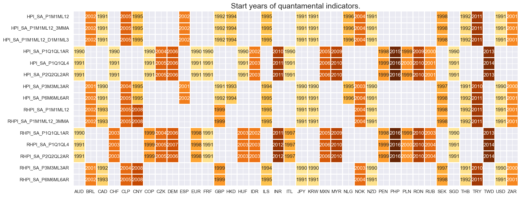
For most countries quantamental information states of residential real estate prices are available from early 1990s. A few emerging market economies have delayed start of the series in 2000s. Late joiners are India (2011), Philippines (2010), Romania (2009), Turkey (2010), and Taiwan (2013).

msm.check_availability(
    df, xcats=main, cids=cids, start_years=True, missing_recent=False
)

Vintage quality is relatively satisfactory even for emerging market economies. There are few exceptions as GBP and KRW, where we use multiple sources to extend the historical coverage.

msp.heatmap_grades(
    df,
    xcats=sorted(hpi),
    cids=cids,
    size=(18, 4),
    title=f"Average vintage grades from {start_date} onwards",
)

For graphical representation below, it is helpful to rename some quarterly dynamics into an equivalent monthly dynamics.

mask = (
    dfd["xcat"].isin([
        "HPI_SA_P1Q1QL4", "HPI_SA_P1Q1QL1AR", "HPI_SA_P2Q2QL2AR", "RHPI_SA_P1Q1QL4", "RHPI_SA_P1Q1QL1AR", "RHPI_SA_P2Q2QL2AR",
    ])
) & (
    dfd["cid"] == "JPY"
)
dfd = dfd.loc[~mask]

dict_repl = {
    "HPI_SA_P1Q1QL4": "HPI_SA_P1M1ML12_3MMA",
    "HPI_SA_P1Q1QL1AR": "HPI_SA_P3M3ML3AR",
    "HPI_SA_P2Q2QL2AR": "HPI_SA_P6M6ML6AR",
    "RHPI_SA_P1Q1QL4": "RHPI_SA_P1M1ML12_3MMA",
    "RHPI_SA_P1Q1QL1AR": "RHPI_SA_P3M3ML3AR",
    "RHPI_SA_P2Q2QL2AR": "RHPI_SA_P6M6ML6AR",
}
for key, value in dict_repl.items():
    dfd["xcat"] = dfd["xcat"].str.replace(key, value)

History

Annual nominal house price growth

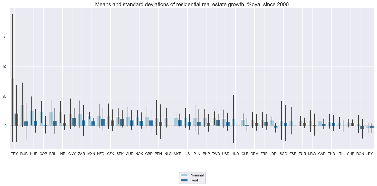
Nominal residential real estate prices have posted very different variances across countries. Generally, countries with higher inflation rates and emerging countries posted larger standard deviations. Real real estate price growth and variation has been more comparable across countries.

cidx = cids_xeu
xcatx = ["HPI_SA_P1M1ML12_3MMA", "RHPI_SA_P1M1ML12_3MMA"]

msp.view_ranges(
    dfd,
    xcats=xcatx,
    cids=cidx,
    sort_cids_by="mean",
    start="1995-01-01",
    kind="bar",
    title="Means and standard deviations of residential real estate growth, %oya, since 2000",
    xcat_labels=["Nominal", "Real"],
    size=(16, 8),
)

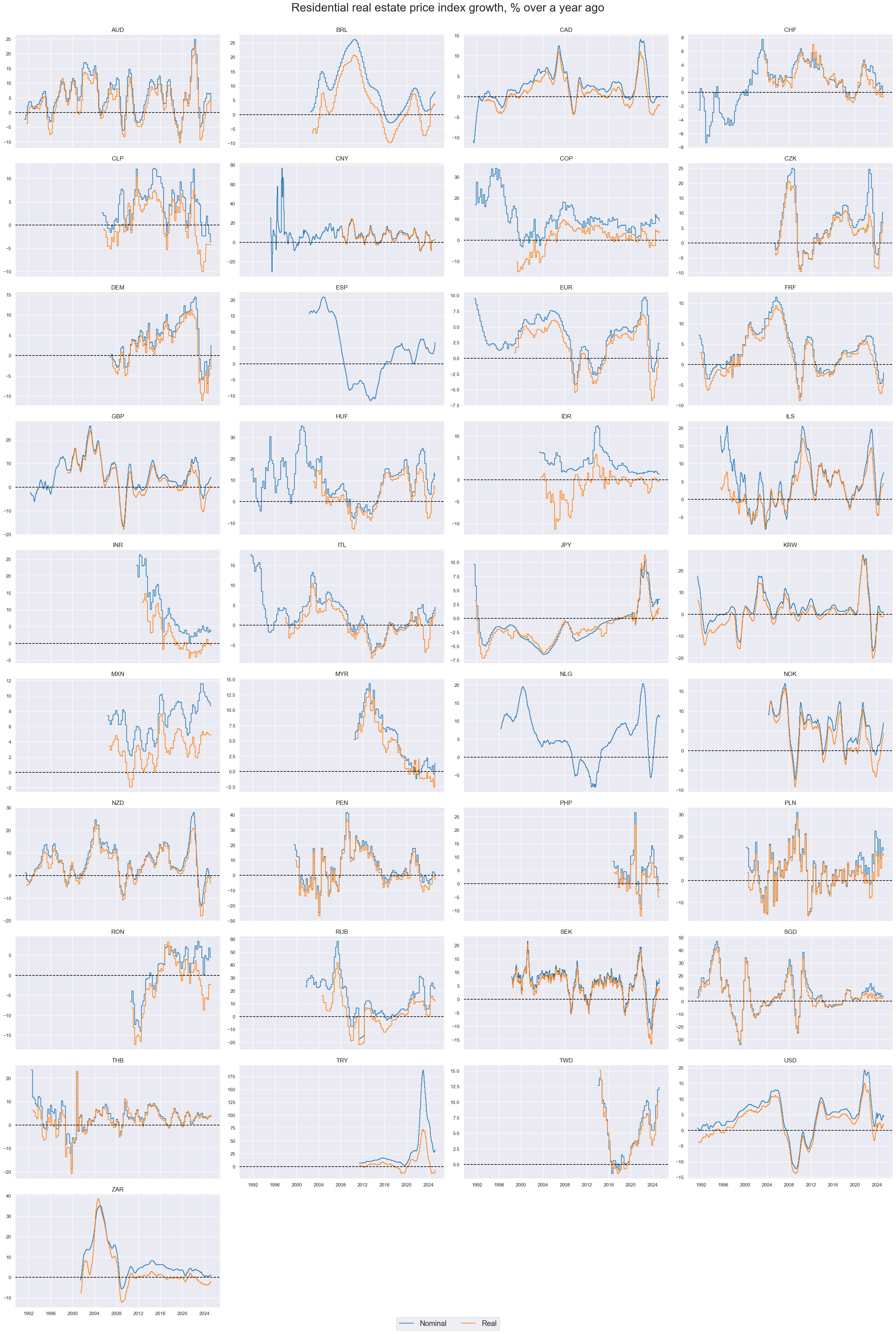
House price growth posted pronounced cycles in the 1990s and 2000s.

cidx = sorted(list(set(cids_xeu) - set(["HKD"])))
xcatx = ["HPI_SA_P1M1ML12_3MMA", "RHPI_SA_P1M1ML12_3MMA"]

msp.view_timelines(
    dfd,
    xcats=xcatx,
    cids=cidx,
    start=start_date,
    title="Residential real estate price index growth, % over a year ago",
    xcat_labels=["Nominal", "Real"],
    ncol=4,
    same_y=False,
    legend_fontsize=17,
    title_fontsize=27,
    size=(12, 7),
    aspect=1.7,
    all_xticks=False,
    legend_ncol=2,
    label_adj=0.05,
)

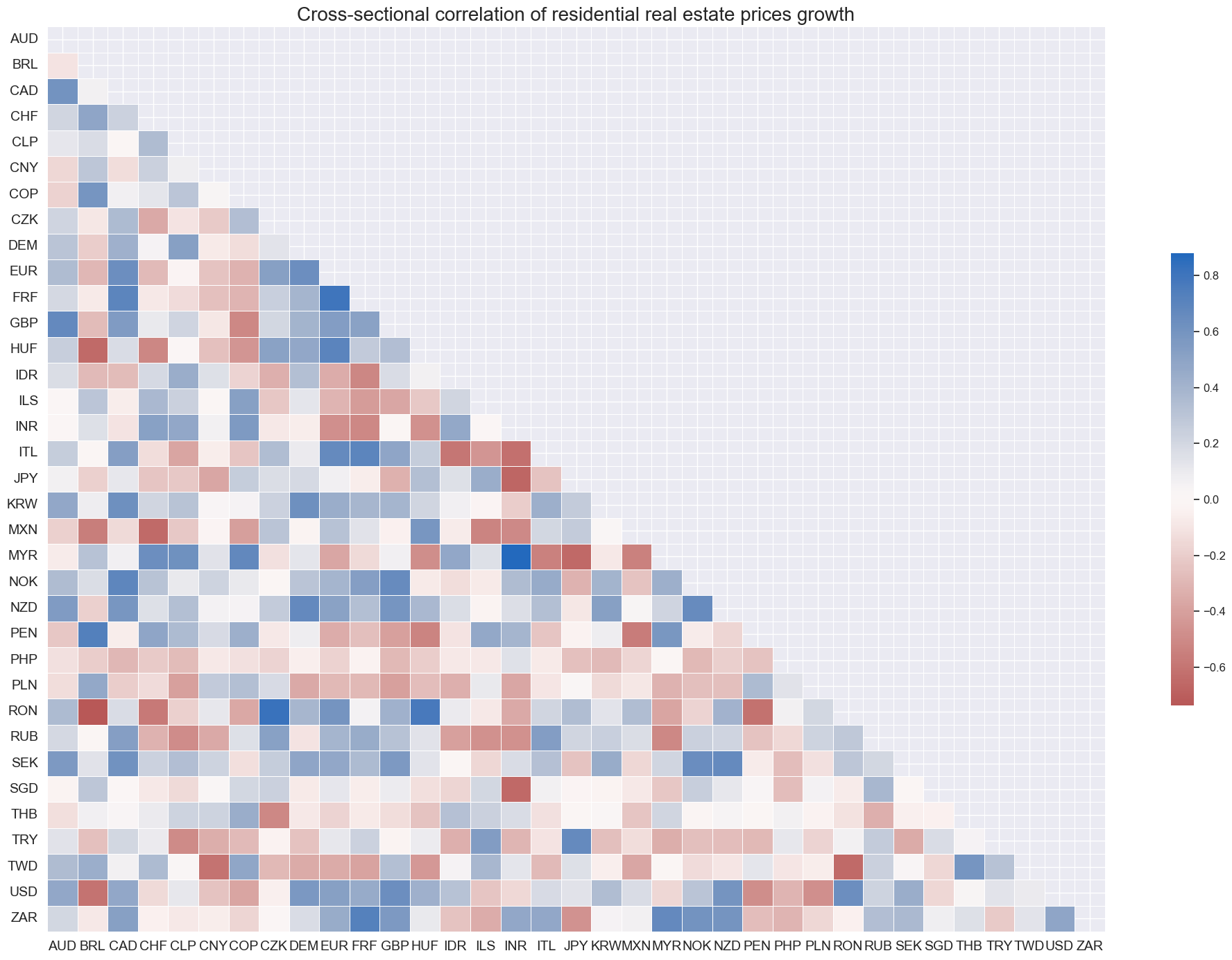
Variation in annual house price has been mostly country-specific, with no clear and strong correlation across all countries considered.

cidx = list(set(cids_xeu) - set(["HKD"]))
msp.correl_matrix(
    dfd,
    xcats="RHPI_SA_P1M1ML12_3MMA",
    cids=cidx,
    size=(20, 14),
    start=start_date,
    title="Cross-sectional correlation of residential real estate prices growth",
    freq="Q"
)

Shorter-term real house price trends

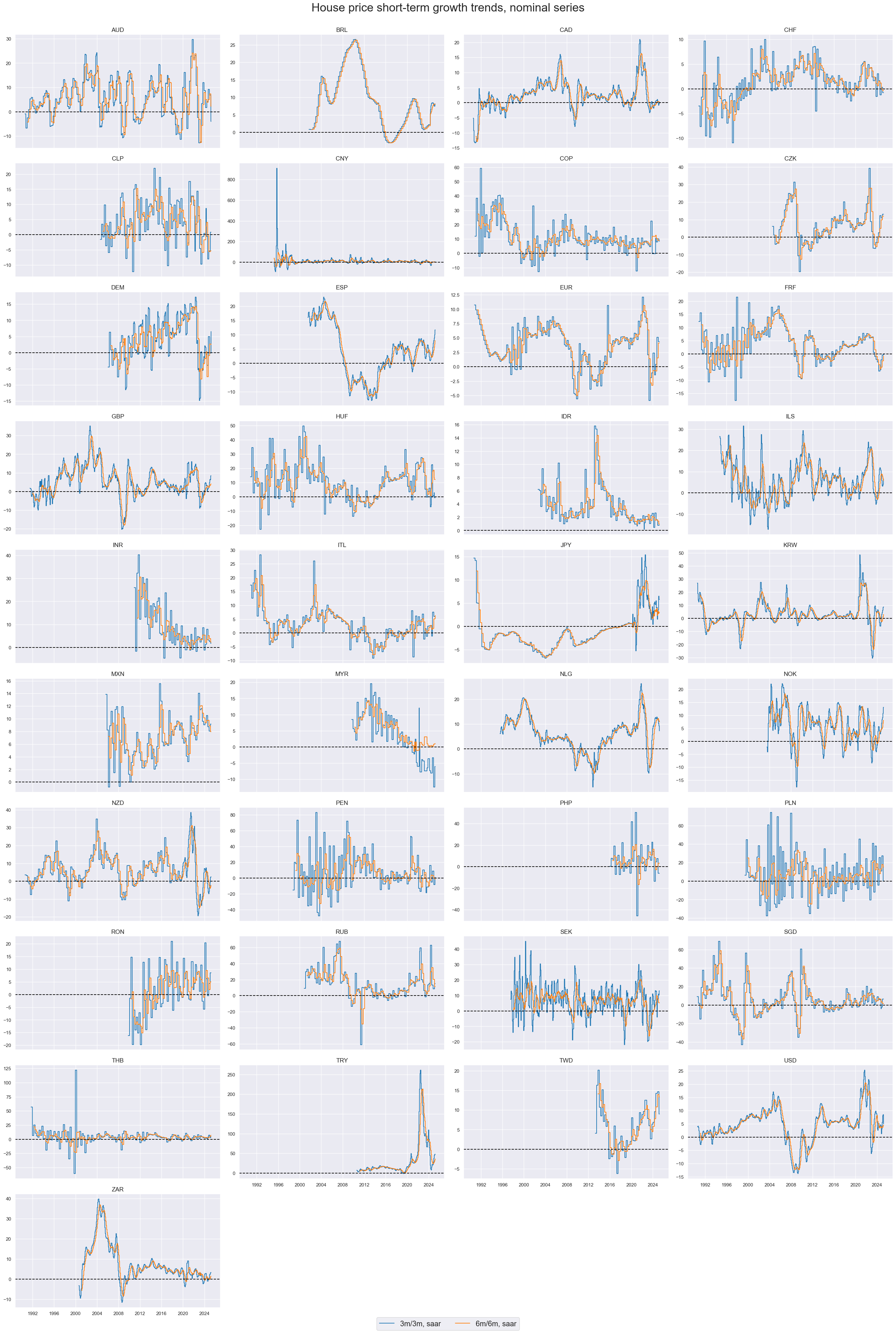
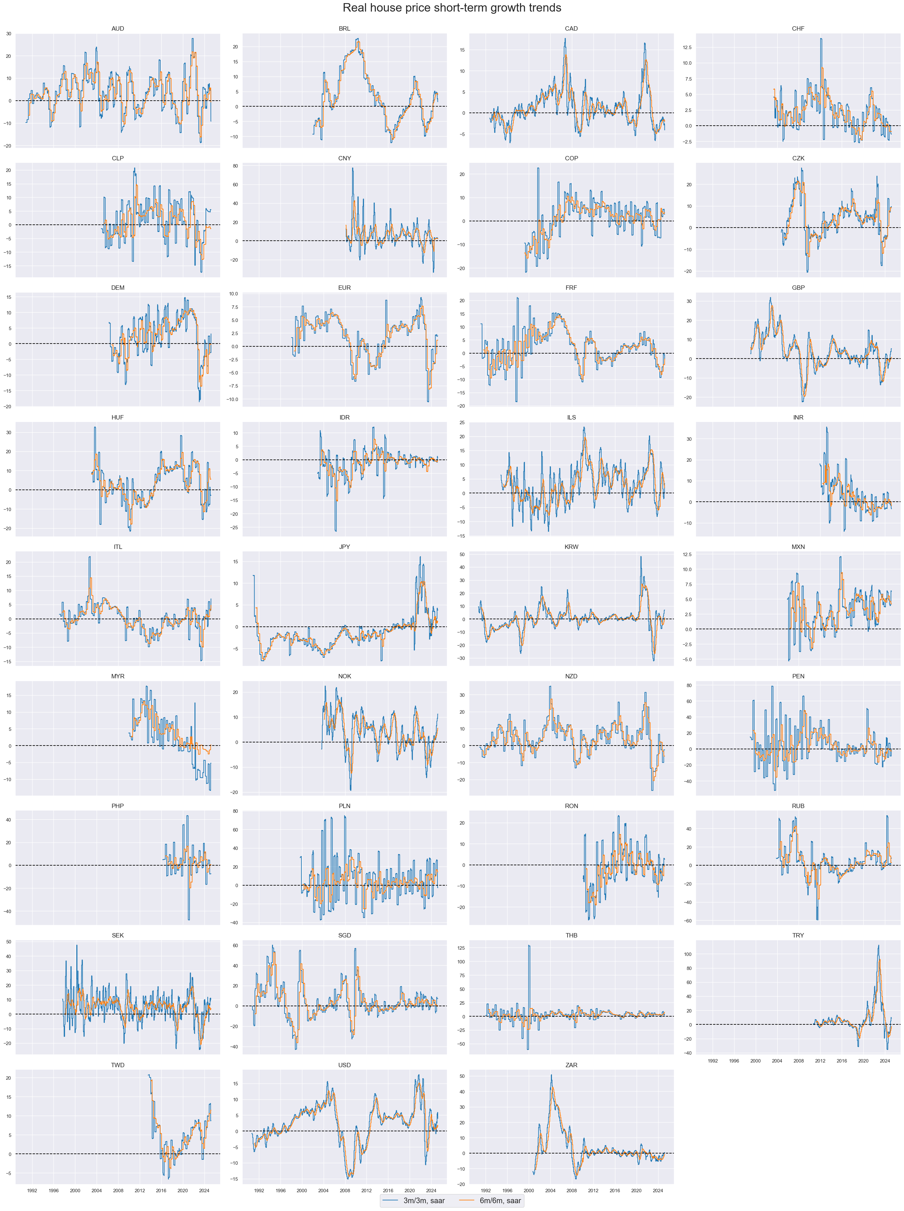
Percent changes based on the past 3 months over the previous 3 months have been quite volatile for most countries. The changes over 6 month periods have been a lot more stable, mainly indicative of trends and cycles in the real estate market.

cidx = sorted(list(set(cids_xeu) - set(["HKD"])))
xcatx = ["HPI_SA_P3M3ML3AR", "HPI_SA_P6M6ML6AR"]

msp.view_timelines(
    dfd,
    xcats=xcatx,
    cids=cidx,
    start=start_date,
    title="House price short-term growth trends, nominal series",
    xcat_labels=[
        "3m/3m, saar",
        "6m/6m, saar",
    ],
    ncol=4,
    same_y=False,
    legend_fontsize=17,
    title_fontsize=27,
    size=(12, 7),
    aspect=1.7,
    all_xticks=False,
    legend_ncol=2,
    label_adj=0.05,
)

cidx = sorted(list(set(cids_xeu) - set(["HKD"])))
xcatx = ["RHPI_SA_P3M3ML3AR", "RHPI_SA_P6M6ML6AR"]

msp.view_timelines(
    dfd,
    xcats=xcatx,
    cids=cidx,
    start=start_date,
    title="Real house price short-term growth trends",
    xcat_labels=[
        "3m/3m, saar",
        "6m/6m, saar",
    ],
    ncol=4,
    same_y=False,
    legend_fontsize=17,
    title_fontsize=27,
    size=(12, 7),
    aspect=1.7,
    all_xticks=False,
    legend_ncol=2,
    label_adj=0.05,
)

Importance

Research links

“Loose monetary conditions lead to booms in real estate lending and house prices’ bubbles; these, in turn, materially heighten the risk of financial crises. Both effects have become stronger in the postwar era.” Jorda et al - Betting the house

“We find that real house prices are pro-cyclical–co-moving with real GDP, consumption, investment, CPI inflation, budget and current account balances, and output gaps. House price booms are typically preceded by a period of easing monetary policy, but then diminishing slack and rising inflation lead monetary authorities to begin tightening policy before house prices peak.” Federal Reserve - Ahearne et al

“House prices respond to monetary policy surprises much more quickly than previously thought, in a matter of weeks rather than years. We show that the key channel for a fast reaction in house prices is the near-immediate adjustment of mortgage rates following monetary policy surprises…” Kudlyak et al

Empirical clues

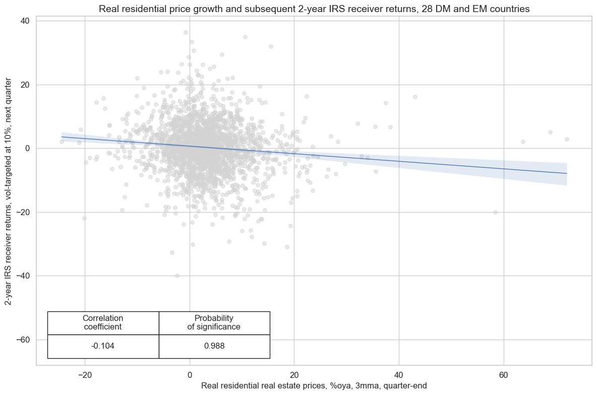
House price booms encourage monetary tightening, while housing price busts often call for monetary easing. Indeed, real house price growth has been significantly and negatively correlated with subsequent interest rate swap fixed receiver returns, particularly in the 2-year segment and at both monthly and quarterly frequencies.

cidx = list(set(cids_xeu) - set(["HKD"]))
xcatx = ["RHPI_SA_P1M1ML12_3MMA", "DU02YXR_VT10"]

cr = msp.CategoryRelations(
    dfd,
    xcats=xcatx,
    cids=cidx,
    freq="Q",
    lag=1,
    xcat_aggs=["last", "sum"],
    fwin=1,
    start="2000-01-01",
    years=None,
    xcat_trims=[100, 100]  # remove two untradable returns
)

cr.reg_scatter(
    title="Real residential price growth and subsequent 2-year IRS receiver returns, 28 DM and EM countries",
    labels=False,
    coef_box="lower left",
    xlab="Real residential real estate prices, %oya, 3mma, quarter-end",
    ylab="2-year IRS receiver returns, vol-targeted at 10%, next quarter",
    prob_est="map",
)

DU02YXR_VT10 misses: ['BRL', 'PEN', 'PHP', 'RON'].

dfx = dfd.loc[:, ["real_date", "cid", "xcat", "value"]]  # reduced dataframe for additions

calcs = [
    f"EQC{sector}vALLR_{tf} = EQC{sector}R_{tf} - EQCALLR_{tf}" 
    for sector in ["FIN"]
    for tf in ["NSA", "VT10"]
]
dfa = msp.panel_calculator(
    dfx, 
    calcs=calcs, 
    cids=cids
)
dfx = msm.update_df(dfx, dfa)

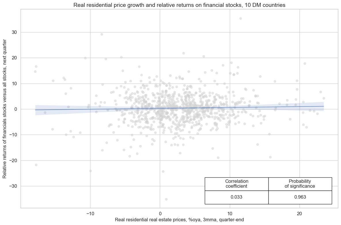
There has also been positive predictive relation of house price growth and subsequent relative returns of financial stocks versus the overall equity market. Significant predictive power shows at the monthly and quarterly frequencies.

cidx = cids_dmca
xcatx = ["RHPI_SA_P1M1ML12_3MMA", "DU02YXR_VT10"]

cr = msp.CategoryRelations(
    dfx,
    xcats=["RHPI_SA_P1M1ML12_3MMA", "EQCFINvALLR_NSA"],
    cids=cidx,
    freq="Q",
    lag=1,
    xcat_aggs=["last", "sum"],
    fwin=1,
    start="2000-01-01",
    years=None,
    xcat_trims=[40, 40], # remove signle outlier for nicer graph
)

cr.reg_scatter(
    title="Real residential price growth and relative returns on financial stocks, 10 DM countries",
    labels=False,
    coef_box="lower right",
    xlab="Real residential real estate prices, %oya, 3mma, quarter-end",
    ylab="Relative returns of financials stocks versus all stocks, next quarter",
    prob_est="map",
)

Appendices

Appendix 1: Currency symbols

The word ‘cross-section’ refers to currencies, currency areas or economic areas. In alphabetical order, these are AUD (Australian dollar), BRL (Brazilian real), CAD (Canadian dollar), CHF (Swiss franc), CLP (Chilean peso), CNY (Chinese yuan renminbi), COP (Colombian peso), CZK (Czech Republic koruna), DEM (German mark), ESP (Spanish peseta), EUR (Euro), FRF (French franc), GBP (British pound), HKD (Hong Kong dollar), HUF (Hungarian forint), IDR (Indonesian rupiah), ITL (Italian lira), JPY (Japanese yen), KRW (Korean won), MXN (Mexican peso), MYR (Malaysian ringgit), NLG (Dutch guilder), NOK (Norwegian krone), NZD (New Zealand dollar), PEN (Peruvian sol), PHP (Phillipine peso), PLN (Polish zloty), RON (Romanian leu), RUB (Russian ruble), SEK (Swedish krona), SGD (Singaporean dollar), THB (Thai baht), TRY (Turkish lira), TWD (Taiwanese dollar), USD (U.S. dollar), ZAR (South African rand).

Appendix 2: Residential real estate details

hpi = pd.DataFrame(
    [
        {     
            "country": "Australia",
            "details": "Nominal prices",
        },
       {     
            "country": "Brazil",
            "details": "Nominal price index, 3 months moving average",
        },
        {
            "country": "Canada",
            "details": "Nominal price index",
        },
        {
            "country": "Switzerland",
            "details": "Average of nominal price index for one-family dwellings and apartments",
        },
        {
            "country": "China",
            "details": "Nominal prices",
        },
        {
            "country": "Chile",
            "details": "Nominal price index, 3 months moving average",
        },
        {
            "country": "Colombia",
            "details": "Nominal price index",
        },
        {
            "country": "Czech Republic",
            "details": "Nominal price index for flats",
        },
        {
            "country": "Germany",
            "details": "Nominal price index",
        },
        {
            "country": "Spain",
            "details": "Nominal price index",
        },
        {
            "country": "Euro Area",
            "details": "Nominal price index",
        },
        {
            "country": "France",
            "details": "Nominal price index excluding overseas territories",
        },
        {
            "country": "Hungary",
            "details": "Nominal price index",
        },
        {
            "country": "India",
            "details": "Nominal price index",
        },
        {
            "country": "Indonesia",
            "details": "Nominal price index",
        },
        {
            "country": "Israel",
            "details": "Nominal price index for urban dwellings",
        },
        {
            "country": "Italy",
            "details": "Nominal price index",
        },
        {
            "country": "Japan",
            "details": "Nominal price index",
        },
        {
            "country": "South Korea",
            "details": "Nominal price index",
        },
        {
            "country": "Malaysia",
            "details": "Nominal price index",
        },
        {
            "country": "Mexico",
            "details": "Nominal price index",
        },
        {
            "country": "Netherlands",
            "details": "Nominal price index for owner-occupied dwellings",
        },
        {
            "country": "New Zealand",
            "details": "Nominal prices",
        },
        {
            "country": "Norway",
            "details": "Nominal price index",
        },
        {
            "country": "Peru",
            "details": "Nominal price index",
        },
        {
            "country": "Philippines",
            "details": "Nominal price index",
        },
        {
            "country": "Poland",
            "details": "Nominal price per square meter index, adjusting by usable floor space",
        },
        {
            "country": "Romania",
            "details": "Nominal price index",
        },
        {
            "country": "Russia",
            "details": "Average growth of nominal prices for primary and secondary market apartments",
        },
        {
            "country": "Sweden",
            "details": "Nominal price index for one- and two-family dwellings",
        },
        {
            "country": "Turkey",
            "details": "Nominal price index",
        },
        {
            "country": "Thailand",
            "details": "Nominal price index",
        },
        {
            "country": "Taiwan",
            "details": "Nominal price index",
        },
        {
            "country": "United Kingdom",
            "details": "Nominal price index, seasonally adjusted",
        },
        {
            "country": "United States",
            "details": "Nominal price index for existing dwellings, using median sale prices",
        },
        {
            "country": "South Africa",
            "details": "Nominal price index",
        },
    ]
)

HTML(hpi.to_html(index=False))

country	details
Australia	Nominal prices
Brazil	Nominal price index, 3 months moving average
Canada	Nominal price index
Switzerland	Average of nominal price index for one-family dwellings and apartments
China	Nominal prices
Chile	Nominal price index, 3 months moving average
Colombia	Nominal price index
Czech Republic	Nominal price index for flats
Germany	Nominal price index
Spain	Nominal price index
Euro Area	Nominal price index
France	Nominal price index excluding overseas territories
Hungary	Nominal price index
India	Nominal price index
Indonesia	Nominal price index
Israel	Nominal price index for urban dwellings
Italy	Nominal price index
Japan	Nominal price index
South Korea	Nominal price index
Malaysia	Nominal price index
Mexico	Nominal price index
Netherlands	Nominal price index for owner-occupied dwellings
New Zealand	Nominal prices
Norway	Nominal price index
Peru	Nominal price index
Philippines	Nominal price index
Poland	Nominal price per square meter index, adjusting by usable floor space
Romania	Nominal price index
Russia	Average growth of nominal prices for primary and secondary market apartments
Sweden	Nominal price index for one- and two-family dwellings
Turkey	Nominal price index
Thailand	Nominal price index
Taiwan	Nominal price index
United Kingdom	Nominal price index, seasonally adjusted
United States	Nominal price index for existing dwellings, using median sale prices
South Africa	Nominal price index