Consistent core CPI trends

This category group contains real-time measures of internationally comparable core consumer price trend indicators. These are based on vintages that are constructed consistently across countries by excluding roughly similar food, fuels and energy items. For many currency areas, the exclusion has been done by the JPMaQS team. Consistent core CPI can be quite different from the local convention of core CPI. Local conventions may include some of these food and energy prices, whilst excluding other items such as administered prices, or simply adjust on statistical grounds.

Consistent core CPI trends are important indicators to measure relative inflation trends across currency areas, which may affect the relative performance of local-currency bond and equity markets.

Annual consistent core CPI inflation

Ticker : CPIXFE_SA_P1M1ML12

Label : Consistent core CPI inflation, %oya

Definition : CPI excluding food and energy components, consistent calculation across countries, % over a year ago

Notes :

• The underlying CPI excludes the following key components across countries: (1) processed and unprocessed food, (2) non-alcoholic beverages, (3) alcoholic beverages, (4) tobacco, (5) fuels for personal transport, and (6) other energy. For countries and periods where categories were not available, proxies have been chosen. For example, the category ‘fuels for personal transport’ was not available for some countries.

• Approximate consistent core CPI indexes are calculated based on monthly changes as explained in Appendix 1 .

• The idea behind this indicator category is to allow for the like-for-like comparison of inflation trends across currency areas. This facilitates, for example, the calculation of meaningful relative inflation trends.

Seasonally and jump-adjusted consistent core CPI trend

Ticker : CPIXFE_SJA_P3M3ML3AR / _P6M6ML6AR

Label : Consistent core CPI trend, seasonally and jump-adjusted: % 3m/3m ar / % 6m/6m ar.

Definition : CPI excluding food and energy components, consistent calculation across countries, seasonally and jump-adjusted: % of latest 3 months over previous 3 months at annualized rate / % of latest 6 months over previous 6 months at an annualized rate.

Notes :

• The underlying CPI excludes the following key components across countries: (1) processed and unprocessed food, (2) non-alcoholic beverages, (3) alcoholic beverages, (4) tobacco, (5) fuels for personal transport, and (6) other energy. For countries and periods where categories were not available, proxies have been chosen. For example, the category ‘fuels for personal transport’ was not available for some countries.

• Approximate consistent core CPI indexes are calculated based on monthly changes as explained in Appendix 1 .

• Jump adjustment means that two types of outliers are adjusted for. First, large “spikes” (i.e. two subsequent large moves of the seasonal index in opposite directions) are averaged. The causes for spikes are often holiday shifts between two months, while the causes for jumps are mostly indirect taxes, administered prices or FX turbulences. Second, large one-off jumps in the index are replaced by the local trend. The criteria for adjustment are statistical based on pattern recognition.

• Jump adjustment is applied to the core CPI inflation series before the final trend measures are calculated.

• Seasonal adjustment factors are sequentially re-estimated as new data are released.

Change in consistent core consumer price inflation

Ticker : CPIXFE_SA_P1M1ML12_D1M1ML3

Label : Change in consistent core consumer price inflation.

Definition : Change in consumer price measure excluding specific food and energy components, % change over a year ago, difference of latest released month compared to three months ago.

Notes :

• The idea behind the indicator is to allow comparing inflation changes across currency areas like-for-like. This facilitates, for example, the calculation of meaningful relative inflation changes.

• The underlying CPI excludes the following key components across countries: (1) processed and unprocessed food, (2) non-alcoholic beverages, (3) alcoholic beverages, (4) tobacco, (5) fuels for personal transport, and (6) other energy. For countries and periods for which categories were not available, proxies have been chosen. For some countries, the category ‘fuels for personal transport’ was not available.

Annual consistent energy inflation

Ticker : CPIE_SA_P1M1ML12 / _P1Q1QL4

Label : Energy CPI inflation, %oya: monthly / quarterly

Definition : Consumer price index for energy components, consistent calculation across countries, % over a year ago: with underlying monthly observations / with underlying quarterly observations

Notes :

• The underlying food CPI includes the following key components across countries: (1) fuels for personal transport, and (2) other energy for households heating. For countries and periods for which categories were not available, proxies have been chosen. For example, the category ‘fuels for personal transport’ was not available for some countries.

• Approximate consistent energy inflation indexes are calculated based on monthly changes as explained in Appendix 1 .

• The idea behind this indicator category is to allow for the like-for-like comparison of inflation trends across currency areas. This facilitates, for example, the calculation of meaningful relative inflation trends.

• CNY indicators are missing due to the lack of detailed CPI basket weights for the individual inputs.

• NZD is the only region reporting quarterly CPI Food and Inflation figures.

Seasonally and jump-adjusted consistent energy inflation trend

Ticker : CPIE_SJA_P3M3ML3AR / _P6M6ML6AR / _P1Q1QL1AR / _P2Q2QL2AR

Label : Energy CPI trend, seasonally and jump-adjusted: % 3m/3m ar / % 6m/6m ar / % 1q/1q ar / % 2q/2q ar.

Definition : Consumer price index for energy components, consistent calculation across countries, seasonally and jump-adjusted: % of latest 3 months over previous 3 months at annualized rate / % of latest 6 months over previous 6 months at an annualized rate / % of latest quarter over previous quarter at annualized rate / % of latest 2 quarters over previous 2 quarters at an annualized rate.

Notes :

• The underlying energy CPI includes the following key components across countries: (1) fuels for personal transport, and (2) other energy for households heating. For countries and periods for which categories were not available, proxies have been chosen. For example, the category ‘fuels for personal transport’ was not available for some countries.

• Approximate consistent core CPI indexes are calculated based on monthly changes as explained in Appendix 1 .

• Jump adjustment means that two types of outliers are adjusted for. First, large “spikes” (i.e. two subsequent large moves of the seasonal index in opposite directions) are averaged. The causes for spikes are often holiday shifts between two months, while the causes for jumps are mostly indirect taxes, administered prices or FX turbulences. Second, large one-off jumps in the index are replaced by the local trend. The criteria for adjustment are statistical based on pattern recognition.

• Jump adjustment is applied to the energy CPI inflation series before the final trend measures are calculated.

• Seasonal adjustment factors are sequentially re-estimated as new data are released.

• CNY indicators are missing due to the lack of detailed CPI basket weights for the individual inputs.

• NZD is the only region reporting quarterly CPI Food and Inflation figures.

Change in consistent energy inflation

Ticker : CPIE_SA_P1M1ML12_D1M1ML3

Label : Change in energy consumer price inflation.

Definition : Change in consumer price measure for energy components, % change over a year ago, difference of latest released month compared to three months ago.

Notes :

• The idea behind the indicator is to allow comparing inflation changes across currency areas like-for-like. This facilitates, for example, the calculation of meaningful relative inflation changes.

• The underlying energy CPI includes the following key components across countries: (1) fuels for personal transport, and (2) other energy for households heating. For countries and periods for which categories were not available, proxies have been chosen.

• CNY indicators are missing due to the lack of detailed CPI basket weights for the individual inputs.

Annual consistent food inflation

Ticker : CPIF_SA_P1M1ML12 / _P1Q1QL4

Label : Food CPI inflation, %oya: monthly / quarterly

Definition : Consumer price index for food components, consistent calculation across countries, % over a year ago: with underlying monthly observations / with underlying quarterly observations

Notes :

• The underlying food CPI includes the following key components across countries: (1) processed and unprocessed food, (2) non-alcoholic beverages, (3) alcoholic beverages, and (4) tobacco. For countries and periods for which categories were not available, proxies have been chosen.

• Approximate consistent food inflation indexes are calculated based on monthly changes as explained in Appendix 1 .

• The idea behind this indicator category is to allow for the like-for-like comparison of inflation trends across currency areas. This facilitates, for example, the calculation of meaningful relative inflation trends.

• CNY indicators are missing due to the lack of detailed CPI basket weights for the individual inputs.

• NZD is the only region reporting quarterly CPI Food and Inflation figures.

Seasonally and jump-adjusted consistent food inflation trend

Ticker : CPIF_SJA_P3M3ML3AR / _P6M6ML6AR / _P1Q1QL1AR / _P2Q2QL2AR

Label : Food CPI trend, seasonally and jump-adjusted: % 3m/3m ar / % 6m/6m ar / % 1q/1q ar / % 2q/2q ar.

Definition : Consumer price index for food components, consistent calculation across countries, seasonally and jump-adjusted: % of latest 3 months over previous 3 months at annualized rate / % of latest 6 months over previous 6 months at an annualized rate / % of latest quarter over previous quarter at annualized rate / % of latest 2 quarters over previous 2 quarters at an annualized rate.

Notes :

• The underlying food CPI includes the following key components across countries: (1) processed and unprocessed food, (2) non-alcoholic beverages, (3) alcoholic beverages, and (4) tobacco. For countries and periods for which categories were not available, proxies have been chosen.

• Approximate consistent core CPI indexes are calculated based on monthly changes as explained in Appendix 1 .

• Jump adjustment means that two types of outliers are adjusted for. First, large “spikes” (i.e. two subsequent large moves of the seasonal index in opposite directions) are averaged. The causes for spikes are often holiday shifts between two months, while the causes for jumps are mostly indirect taxes, administered prices or FX turbulences. Second, large one-off jumps in the index are replaced by the local trend. The criteria for adjustment are statistical based on pattern recognition.

• Jump adjustment is applied to the food CPI inflation series before the final trend measures are calculated.

• Seasonal adjustment factors are sequentially re-estimated as new data are released.

• CNY indicators are missing due to the lack of detailed CPI basket weights for the individual inputs.

• NZD is the only region reporting quarterly CPI Food and Inflation figures.

Change in consistent food inflation

Ticker : CPIF_SA_P1M1ML12_D1M1ML3

Label : Change in food consumer price inflation.

Definition : Change in consumer price measure for food components, % change over a year ago, difference of latest released month compared to three months ago.

Notes :

• The idea behind the indicator is to allow comparing inflation changes across currency areas like-for-like. This facilitates, for example, the calculation of meaningful relative inflation changes.

• The underlying food CPI includes the following key components across countries: (1) processed and unprocessed food, (2) non-alcoholic beverages, (3) alcoholic beverages, and (4) tobacco. For countries and periods for which categories were not available, proxies have been chosen.

• CNY indicators are missing due to the lack of detailed CPI basket weights for the individual inputs.

Imports

Only the standard Python data science packages and the specialized macrosynergy package are needed.

import os
import numpy as np
import pandas as pd
import matplotlib.pyplot as plt
import numpy as np

import macrosynergy.management as msm
import macrosynergy.panel as msp
import macrosynergy.signal as mss
import macrosynergy.pnl as msn
import macrosynergy.visuals as msv

from macrosynergy.download import JPMaQSDownload

import warnings
warnings.simplefilter("ignore")

The JPMaQS indicators we consider are downloaded using the J.P. Morgan Dataquery API interface within the macrosynergy package. This is done by specifying ticker strings , formed by appending an indicator category code <category> to a currency area code <cross_section> . These constitute the main part of a full quantamental indicator ticker, taking the form DB(JPMAQS,<cross_section>_<category>,<info>) , where <info> denotes the time series of information for the given cross-section and category. The following types of information are available:

• value giving the latest available values for the indicator

• eop_lag referring to days elapsed since the end of the observation period

• mop_lag referring to the number of days elapsed since the mean observation period

• grade denoting a grade of the observation, giving a metric of real time information quality.

After instantiating the JPMaQSDownload class within the macrosynergy.download module, one can use the download(tickers,start_date,metrics) method to easily download the necessary data, where tickers is an array of ticker strings, start_date is the first collection date to be considered and metrics is an array comprising the times series information to be downloaded.

# Cross-sections of interest

cids_dmca = [
    "AUD",
    "CAD",
    "CHF",
    "EUR",
    "GBP",
    "JPY",
    "NOK",
    "NZD",
    "SEK",
    "USD",
]  # DM currency areas
cids_dmec = ["DEM", "ESP", "FRF", "ITL"]  # DM euro area countries
cids_latm = ["BRL", "COP", "CLP", "MXN", "PEN"]  # Latam countries
cids_emea = ["CZK", "HUF", "ILS", "PLN", "RON", "RUB", "TRY", "ZAR"]  # EMEA countries
cids_emas = [
    "CNY",
    "IDR",
    "INR",
    "KRW",
    "MYR",
    "PHP",
    "SGD",
    "THB",
    "TWD",
]  # EM Asia countries

cids_dm = cids_dmca + cids_dmec
cids_em = cids_latm + cids_emea + cids_emas

cids = sorted(cids_dm + cids_em)
cids_exp = sorted(list(set(cids) - set(cids_dmec)))  # cids expected in category panels

# # For bonds and IRS analyses
cids_bond=['AUD', 'DEM', 'ESP', 'FRF', 'GBP', 'ITL', 'JPY', 'NZD', 'USD'] #  al available government bond returns cross-sections
cids_noirs = ['BRL', 'PEN', 'PHP', 'RON']
cids_irs = list(set(cids_exp) - set(cids_noirs))
# For equity analysis
cids_eq = ["AUD", "CAD", "CHF", "EUR", "GBP", "ILS", "JPY", "NOK", "NZD", "SEK", "SGD", "USD"]

# For FX analyses
cids_nofx = ["USD", "EUR", "CNY", "SGD"]
cids_fx = list(set(cids_dmca + cids_em) - set(cids_nofx))
cids_dmfx = list(set(cids_dmca) - set(cids_nofx))
cids_emfx = list(set(cids_em) - set(cids_nofx))

# Quantamental categories of interest

main = [
    "CPIXFE_SA_P1M1ML12",
    "CPIXFE_SJA_P3M3ML3AR",
    "CPIXFE_SJA_P6M6ML6AR",
    "CPIXFE_SA_P1M1ML12_D1M1ML3",
    
    "CPIE_SA_P1M1ML12",
    "CPIE_SJA_P3M3ML3AR",
    "CPIE_SJA_P6M6ML6AR",
    "CPIE_SA_P1M1ML12_D1M1ML3",
    
    "CPIE_SA_P1Q1QL4",
    "CPIE_SJA_P1Q1QL1AR",
    "CPIE_SJA_P2Q2QL2AR",

    "CPIF_SA_P1M1ML12",
    "CPIF_SJA_P3M3ML3AR",
    "CPIF_SJA_P6M6ML6AR",
    "CPIF_SA_P1M1ML12_D1M1ML3",

    "CPIF_SA_P1Q1QL4",
    "CPIF_SJA_P1Q1QL1AR",
    "CPIF_SJA_P2Q2QL2AR",
]
econ = [
    "CPIC_SA_P1M1ML12",
    "CPIC_SJA_P3M3ML3AR",
    "CPIC_SJA_P6M6ML6AR",
    "CPIC_SA_P1M1ML12_D1M1ML3",
   
]  # economic context

misc = ["INFTEFF_NSA", "INFTARGET_NSA"] # Inflation targets 
mark = [
    "DU02YXR_VT10", "DU05YXR_VT10", "FXXR_VT10", "GB05YR_NSA",
    "EQCENRR_NSA", "EQCCOSR_NSA", "EQCALLR_NSA",
]  # market links

xcats = main + econ + mark + misc

# Download series from J.P. Morgan DataQuery by tickers

start_date = "1995-01-01"
tickers = [cid + "_" + xcat for cid in cids for xcat in xcats]
print(f"Maximum number of tickers is {len(tickers)}")

# Retrieve credentials

client_id: str = os.getenv("DQ_CLIENT_ID")
client_secret: str = os.getenv("DQ_CLIENT_SECRET")

# Download from DataQuery

with JPMaQSDownload(client_id=client_id, client_secret=client_secret) as downloader:
    
    df = downloader.download(
        tickers=tickers,
        start_date=start_date,
        metrics=["all"],
        suppress_warning=True,
        show_progress=True,
    )
    

Maximum number of tickers is 1116
Downloading data from JPMaQS.
Timestamp UTC:  2024-07-15 09:08:13
Connection successful!

Requesting data: 100%|███████████████████████████████████████████████████████████████| 224/224 [00:51<00:00,  4.39it/s]
Downloading data: 100%|██████████████████████████████████████████████████████████████| 224/224 [00:38<00:00,  5.89it/s]

Some expressions are missing from the downloaded data. Check logger output for complete list.
1456 out of 4464 expressions are missing. To download the catalogue of all available expressions and filter the unavailable expressions, set `get_catalogue=True` in the call to `JPMaQSDownload.download()`.
Some dates are missing from the downloaded data. 
2 out of 7708 dates are missing.

Availability

msm.missing_in_df(df, xcats=main, cids=cids_exp)

Show code cell output Hide code cell output

No missing XCATs across DataFrame.
Missing cids for CPIE_SA_P1M1ML12:            ['CNY', 'NZD']
Missing cids for CPIE_SA_P1M1ML12_D1M1ML3:    ['CNY', 'NZD']
Missing cids for CPIE_SA_P1Q1QL4:             ['AUD', 'BRL', 'CAD', 'CHF', 'CLP', 'CNY', 'COP', 'CZK', 'EUR', 'GBP', 'HUF', 'IDR', 'ILS', 'INR', 'JPY', 'KRW', 'MXN', 'MYR', 'NOK', 'PEN', 'PHP', 'PLN', 'RON', 'RUB', 'SEK', 'SGD', 'THB', 'TRY', 'TWD', 'USD', 'ZAR']
Missing cids for CPIE_SJA_P1Q1QL1AR:          ['AUD', 'BRL', 'CAD', 'CHF', 'CLP', 'CNY', 'COP', 'CZK', 'EUR', 'GBP', 'HUF', 'IDR', 'ILS', 'INR', 'JPY', 'KRW', 'MXN', 'MYR', 'NOK', 'PEN', 'PHP', 'PLN', 'RON', 'RUB', 'SEK', 'SGD', 'THB', 'TRY', 'TWD', 'USD', 'ZAR']
Missing cids for CPIE_SJA_P2Q2QL2AR:          ['AUD', 'BRL', 'CAD', 'CHF', 'CLP', 'CNY', 'COP', 'CZK', 'EUR', 'GBP', 'HUF', 'IDR', 'ILS', 'INR', 'JPY', 'KRW', 'MXN', 'MYR', 'NOK', 'PEN', 'PHP', 'PLN', 'RON', 'RUB', 'SEK', 'SGD', 'THB', 'TRY', 'TWD', 'USD', 'ZAR']
Missing cids for CPIE_SJA_P3M3ML3AR:          ['CNY', 'NZD']
Missing cids for CPIE_SJA_P6M6ML6AR:          ['CNY', 'NZD']
Missing cids for CPIF_SA_P1M1ML12:            ['CNY', 'NZD']
Missing cids for CPIF_SA_P1M1ML12_D1M1ML3:    ['CNY', 'NZD']
Missing cids for CPIF_SA_P1Q1QL4:             ['AUD', 'BRL', 'CAD', 'CHF', 'CLP', 'CNY', 'COP', 'CZK', 'EUR', 'GBP', 'HUF', 'IDR', 'ILS', 'INR', 'JPY', 'KRW', 'MXN', 'MYR', 'NOK', 'PEN', 'PHP', 'PLN', 'RON', 'RUB', 'SEK', 'SGD', 'THB', 'TRY', 'TWD', 'USD', 'ZAR']
Missing cids for CPIF_SJA_P1Q1QL1AR:          ['AUD', 'BRL', 'CAD', 'CHF', 'CLP', 'CNY', 'COP', 'CZK', 'EUR', 'GBP', 'HUF', 'IDR', 'ILS', 'INR', 'JPY', 'KRW', 'MXN', 'MYR', 'NOK', 'PEN', 'PHP', 'PLN', 'RON', 'RUB', 'SEK', 'SGD', 'THB', 'TRY', 'TWD', 'USD', 'ZAR']
Missing cids for CPIF_SJA_P2Q2QL2AR:          ['AUD', 'BRL', 'CAD', 'CHF', 'CLP', 'CNY', 'COP', 'CZK', 'EUR', 'GBP', 'HUF', 'IDR', 'ILS', 'INR', 'JPY', 'KRW', 'MXN', 'MYR', 'NOK', 'PEN', 'PHP', 'PLN', 'RON', 'RUB', 'SEK', 'SGD', 'THB', 'TRY', 'TWD', 'USD', 'ZAR']
Missing cids for CPIF_SJA_P3M3ML3AR:          ['CNY', 'NZD']
Missing cids for CPIF_SJA_P6M6ML6AR:          ['CNY', 'NZD']
Missing cids for CPIXFE_SA_P1M1ML12:          []
Missing cids for CPIXFE_SA_P1M1ML12_D1M1ML3:  []
Missing cids for CPIXFE_SJA_P3M3ML3AR:        []
Missing cids for CPIXFE_SJA_P6M6ML6AR:        []

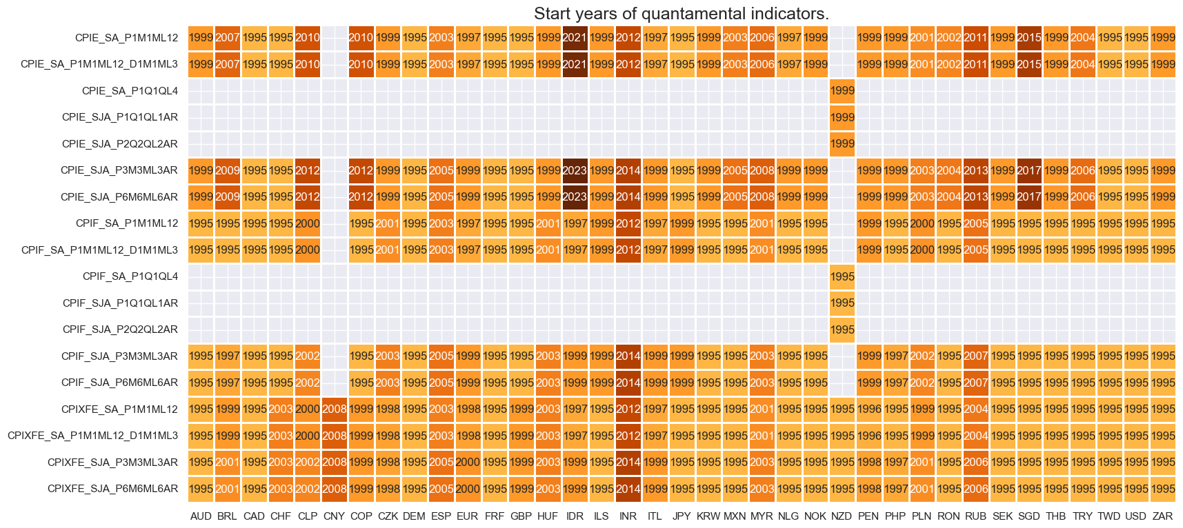
Real-time quantamental indicators of consumer price trends for developed markets are typically available by the late 1990s. Swiss core inflation only starts in 2003, however. The EM series mostly begin in the late 1990s or early 2000s. India is a notable late starter, as CPI was not widely followed before the 2010s.

For the explanation of currency symbols, which are related to currency areas or countries for which categories are available, please view Appendix 2 .

xcatx = main

dfx = msm.reduce_df(df, xcats=xcatx, cids=cids_exp)
dfs = msm.check_startyears(
    dfx,
)
msm.visual_paneldates(dfs, size=(20, 3))

plot = msm.check_availability(
    df, xcats=main, cids=cids_exp, start_size=(20, 2), start_years=False
)

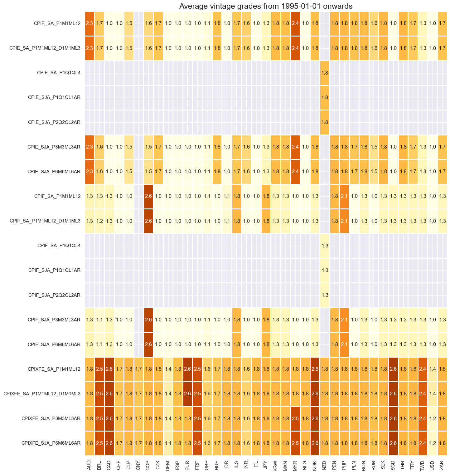
Average grades are currently quite mixed across countries and times.

plot = msp.heatmap_grades(
    df,
    xcats=main,
    cids=cids_exp,
    size=(19, 2),
    title=f"Average vintage grades from {start_date} onwards",
)

xcatx = ["CPIXFE_SA_P1M1ML12", "CPIE_SA_P1M1ML12", "CPIF_SA_P1M1ML12"]
msp.view_ranges(
    df,
    xcats=xcatx,
    cids=cids_exp,
    val="eop_lag",
    title="End of observation period lags (ranges of time elapsed since end of observation period in days)",
    start=start_date,
    kind="box",
    size=(16, 4),
)
msp.view_ranges(
    df,
    xcats=xcatx,
    cids=cids_exp,
    val="mop_lag",
    title="Median of observation period lags (ranges of time elapsed since middle of observation period in days)",
    start=start_date,
    kind="box",
    size=(16, 4),
)

xcatx = ["CPIXFE_SJA_P3M3ML3AR", "CPIE_SJA_P3M3ML3AR", "CPIF_SJA_P3M3ML3AR"]
msp.view_ranges(
    df,
    xcats=xcatx,
    cids=cids_exp,
    val="eop_lag",
    title="End of observation period lags (ranges of time elapsed since end of observation period in days)",
    start=start_date,
    kind="box",
    size=(16, 4),
)
msp.view_ranges(
    df,
    xcats=xcatx,
    cids=cids_exp,
    val="mop_lag",
    title="Median of observation period lags (ranges of time elapsed since middle of observation period in days)",
    start=start_date,
    kind="box",
    size=(16, 4),
)

History

Annual consistent core CPI inflation

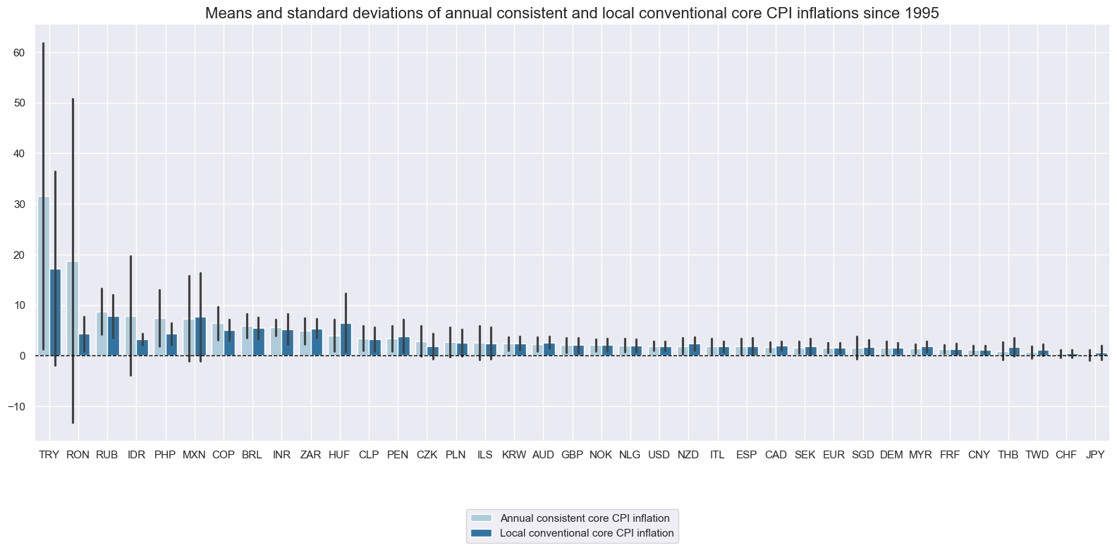
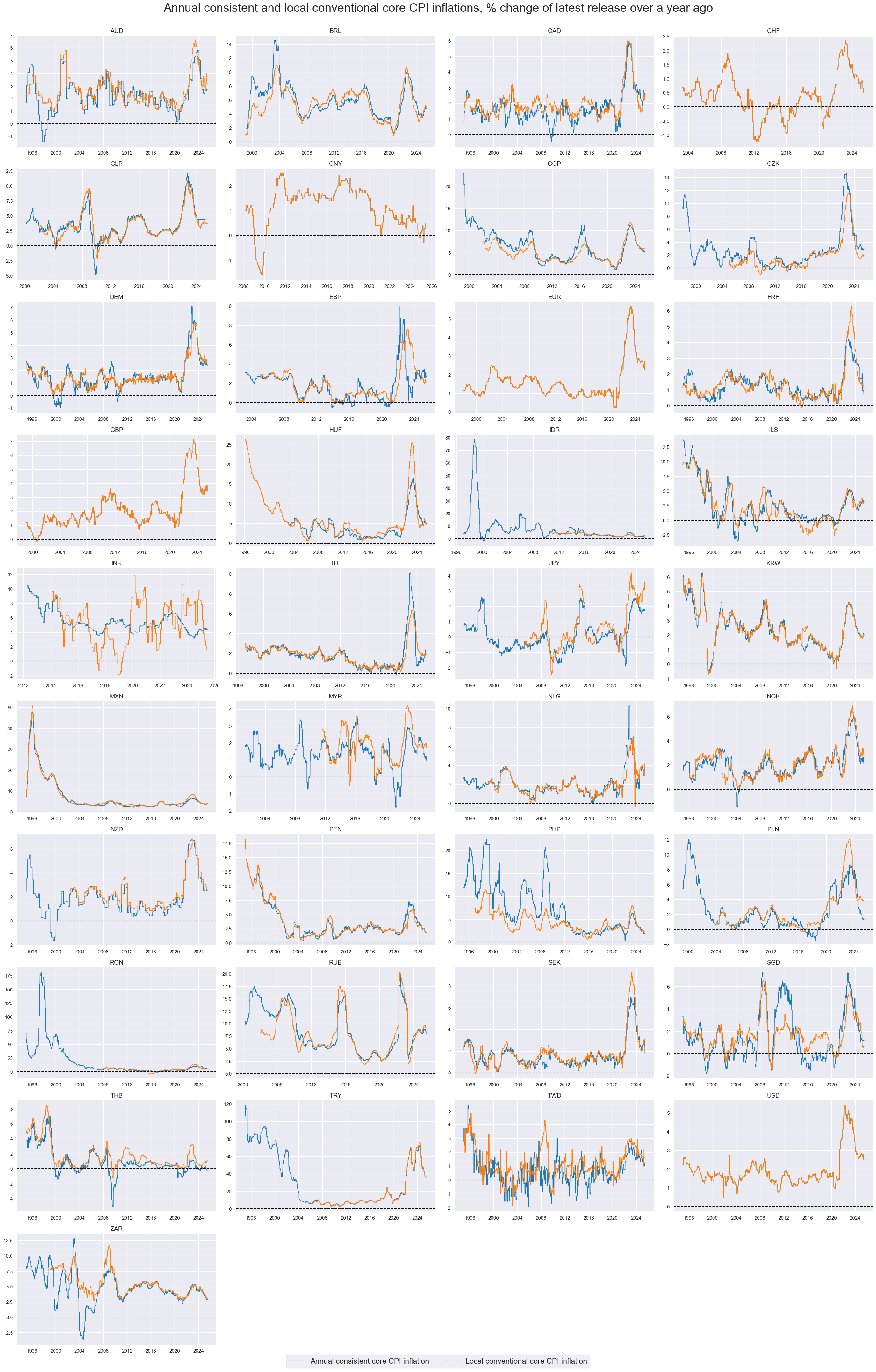
Quantamental indicators of consistent core inflation, measured as % over a year ago, have posted pronounced cycles and trends. For most countries, they have been similar to JPMaQS indicators of conventional core inflation, but there have also been notable differences.

While consistent core CPI excludes only specific food and energy prices, conventional core CPI often excludes prices or uses methods that are of particular local relevance. This explains wide divergences between conventional and consistent core CPI trends in some countries.

xcatx = ["CPIXFE_SA_P1M1ML12", "CPIC_SA_P1M1ML12"]

msp.view_ranges(
    df,
    xcats=xcatx,
    cids=cids_exp,
    sort_cids_by="mean",
    start=start_date,
    kind="bar",
    size=(16, 8),
    title="Means and standard deviations of annual consistent and local conventional core CPI inflations since 1995",
    xcat_labels=[
        "Annual consistent core CPI inflation",
        "Local conventional core CPI inflation",
    ],
)

xcatx = ["CPIXFE_SA_P1M1ML12", "CPIC_SA_P1M1ML12"]

msp.view_timelines(
    df,
    xcats=xcatx,
    cids=cids_exp,
    start=start_date,
    title="Annual consistent and local conventional core CPI inflations, % change of latest release over a year ago",
    xcat_labels=[
        "Annual consistent core CPI inflation",
        "Local conventional core CPI inflation",
    ],
    legend_fontsize=17,
    title_fontsize=27,
    ncol=4,
    same_y=False,
    size=(16, 8),
    all_xticks=True,
)

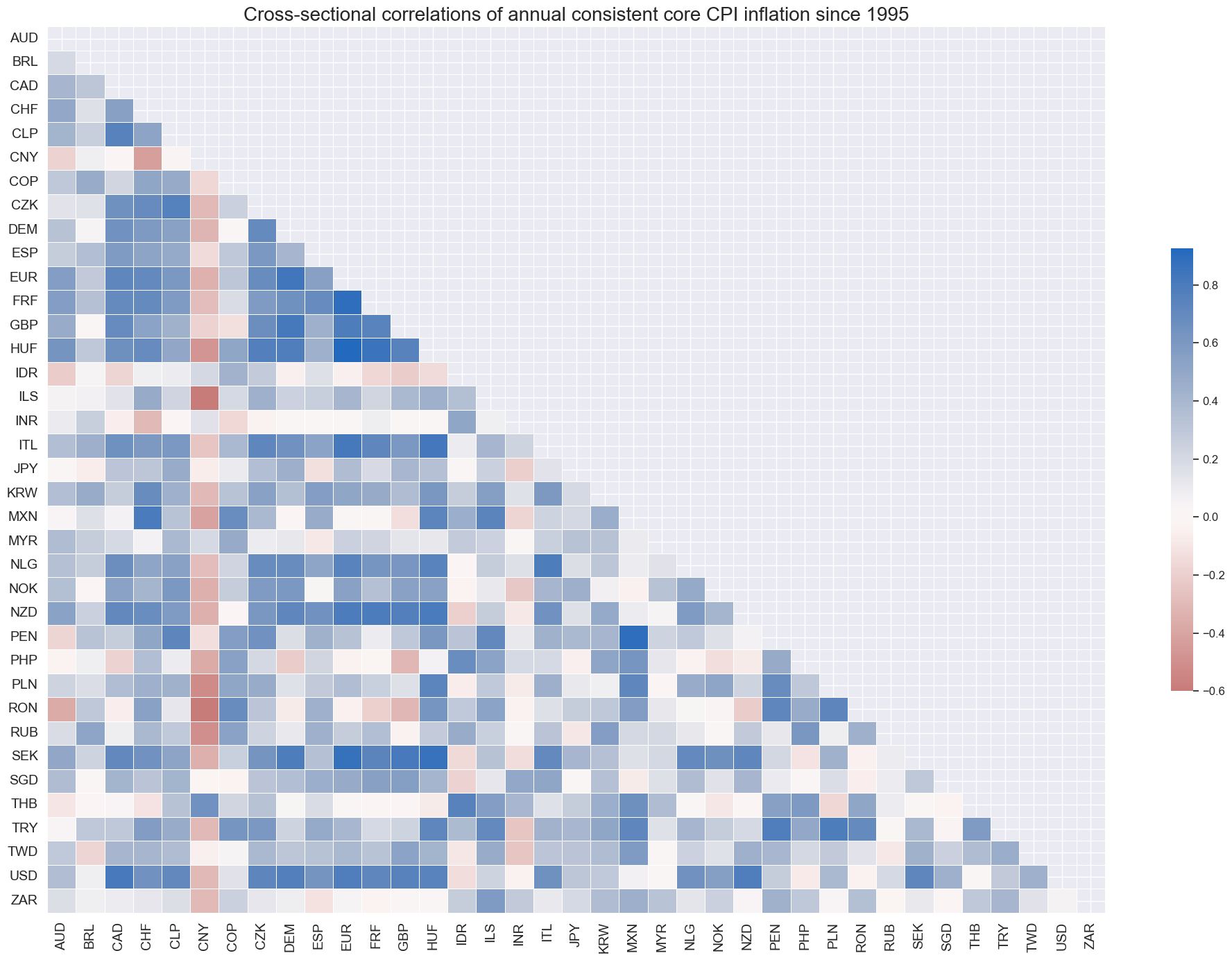
Unlike for conventional CPI measures, cross-country correlations of consistent core CPI have not always been positive, emphasizing that this metric focuses more on local inflation trends and less on global effects, such as commodity price fluctuations and harvest conditions. This makes consistent core inflation a suitable basis for detecting inflation trend differentials.

msp.correl_matrix(
    df,
    xcats= ["CPIXFE_SA_P1M1ML12"],
    cids=cids_exp,
    size=(20, 14),
    title="Cross-sectional correlations of annual consistent core CPI inflation since 1995",
)

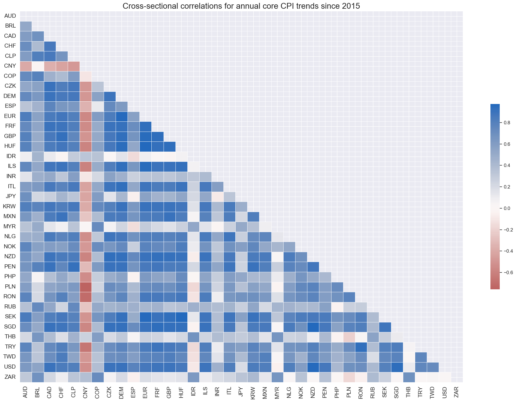
Since 2015, China has stood out as the one country maintaining a negative correlation with global consistent core CPI growth.

msp.correl_matrix(
    df,
    xcats="CPIXFE_SA_P1M1ML12",
    cids=cids_exp,
    title="Cross-sectional correlations for annual core CPI trends since 2015",
    start="2015-01-01",
    size=(20, 14),
)

Adjusted consistent core CPI trends

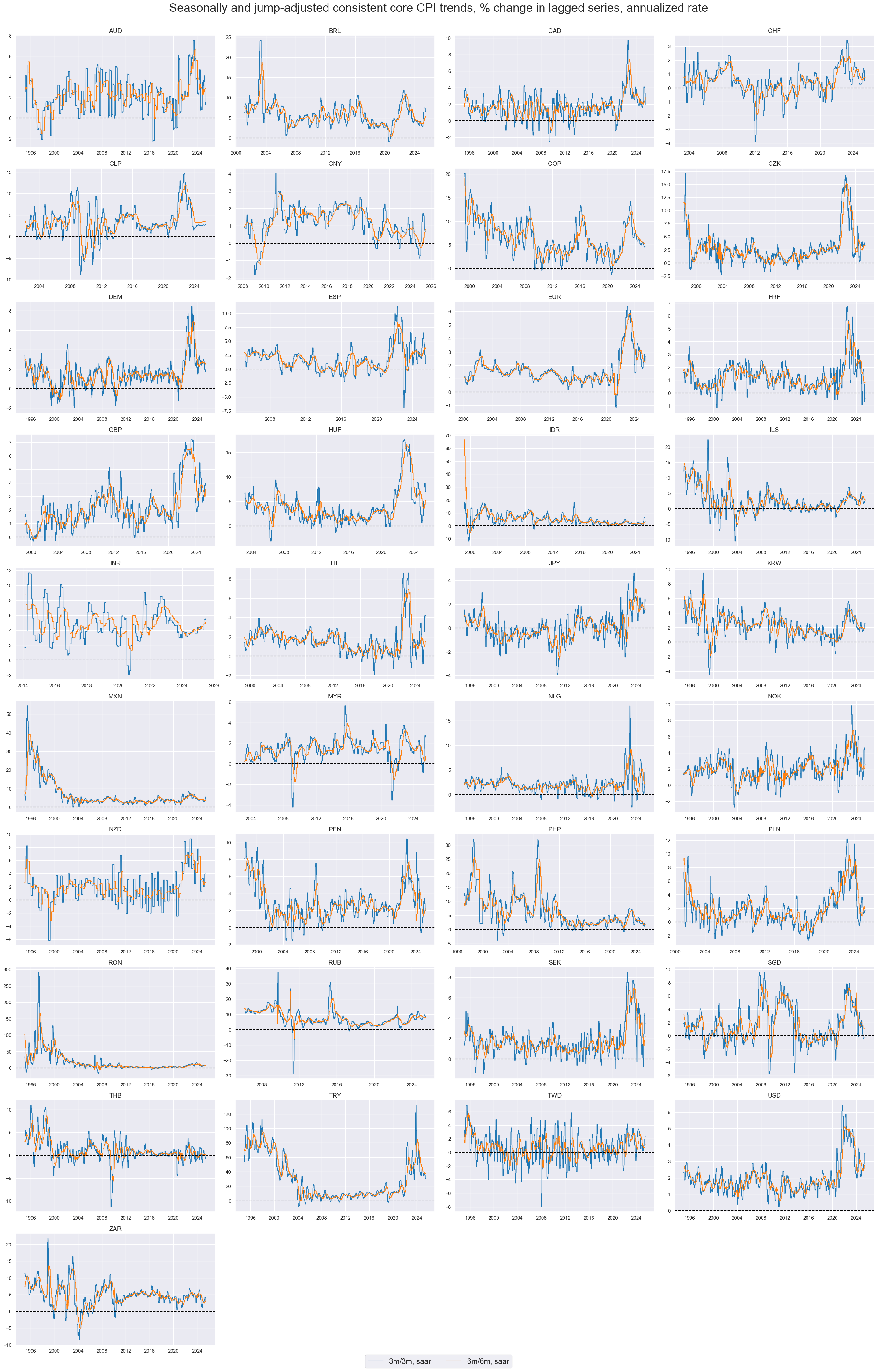
The 6-months-over-6-months trends exhibit greater stability than the 3-months-over-3-months trends and seem to be a useful basis for measuring shorter-term inflation trend differentials across countries.

xcatx = ["CPIXFE_SJA_P3M3ML3AR", "CPIXFE_SJA_P6M6ML6AR"]

msp.view_timelines(
    df,
    xcats=xcatx,
    cids=cids_exp,
    start=start_date,
    title="Seasonally and jump-adjusted consistent core CPI trends, % change in lagged series, annualized rate",
    xcat_labels=[
        "3m/3m, saar",
        "6m/6m, saar",
    ],
    legend_fontsize=17,
    title_fontsize=27,
    ncol=4,
    same_y=False,
    all_xticks=True,
)

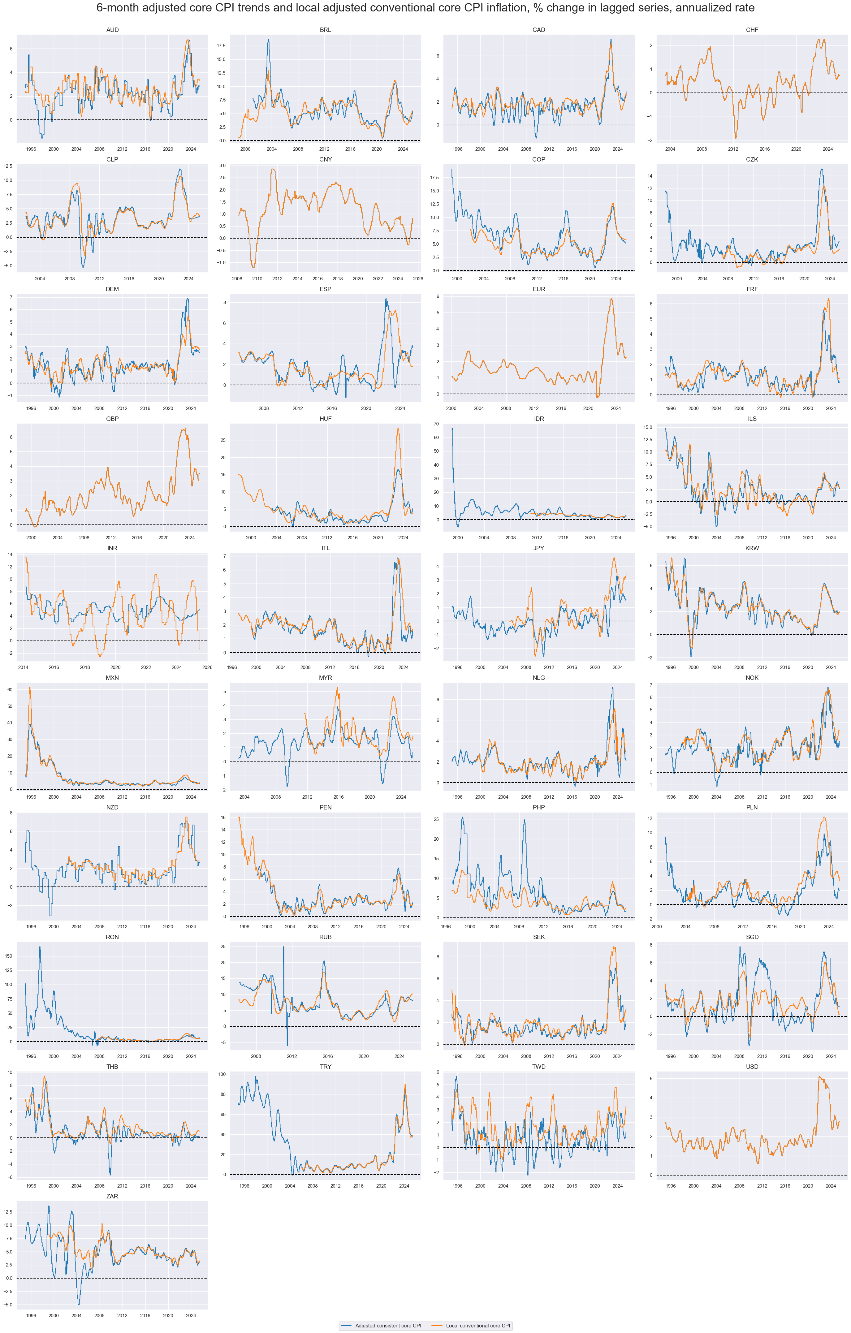
Consistent core CPI trends are often, but not always, more volatile than local conventional core inflation metrics. After all, there is a reason why countries exclude specific items from their inflation measurement.

xcatx = ["CPIXFE_SJA_P6M6ML6AR", "CPIC_SJA_P6M6ML6AR"]

msp.view_timelines(
    df,
    xcats=xcatx,
    cids=cids_exp,
    start=start_date,
    title="6-month adjusted core CPI trends and local adjusted conventional core CPI inflation, % change in lagged series, annualized rate",
    xcat_labels=[
        "Adjusted consistent core CPI",
        "Local conventional core CPI",
    ],
    title_fontsize=27,
    ncol=4,
    same_y=False,
    all_xticks=True,
)

Change in consistent core consumer price inflation

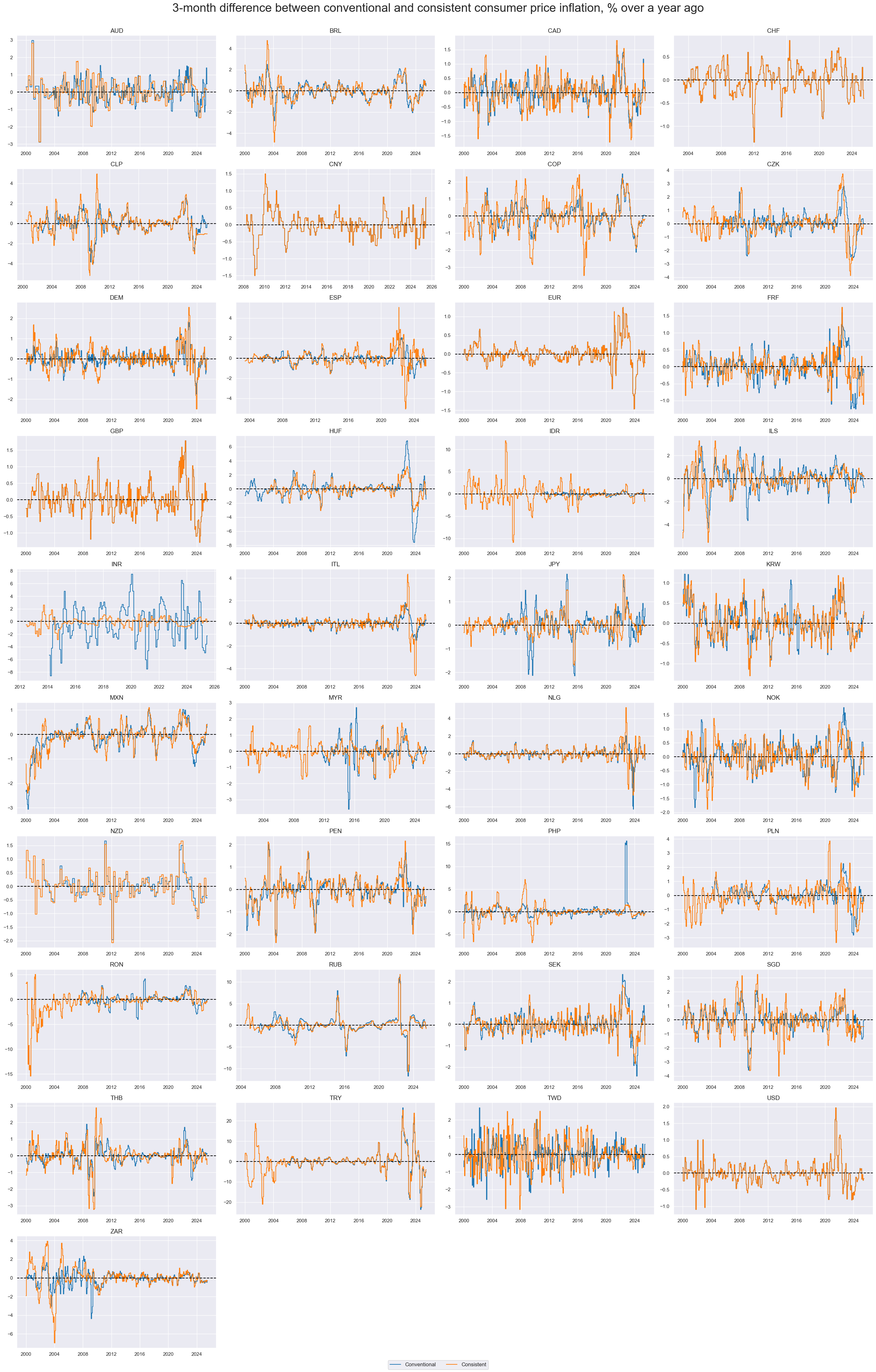
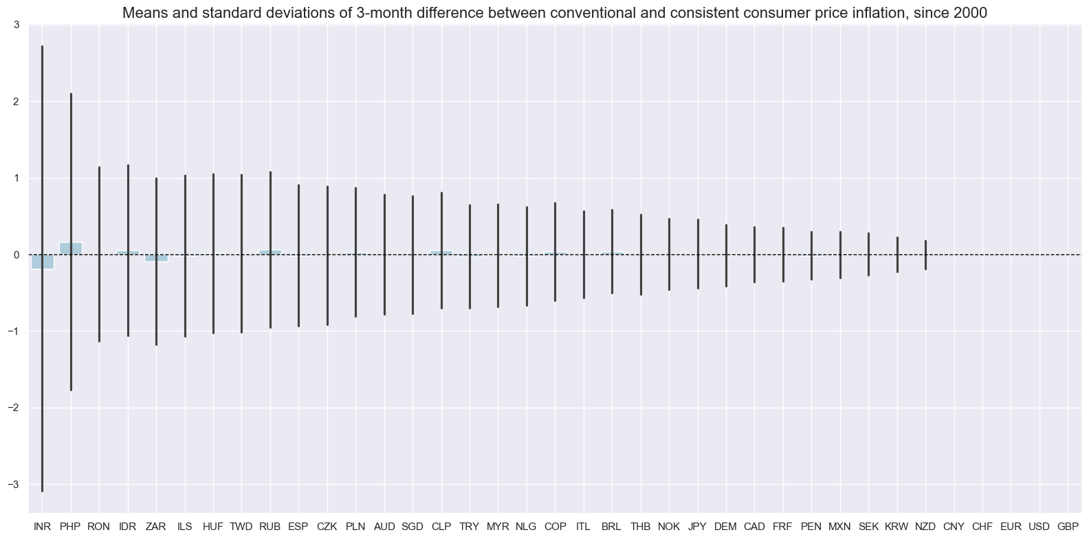
The dynamics of consistent core CPI changes and core inflation changes (according to local convention) have been very different across sleected countries.

xcatx = ["CPIC_SA_P1M1ML12_D1M1ML3", "CPIXFE_SA_P1M1ML12_D1M1ML3"]

msp.view_timelines(
    df,
    xcats=xcatx,
    cids=cids_exp,
    start="2000-01-01",
    title="3-month difference between conventional and consistent consumer price inflation, % over a year ago",
    title_fontsize=27,
    xcat_labels=["Conventional", "Consistent"],
    ncol=4,
    same_y=False,
    all_xticks=True,
)

calcs = ["Conv_vs_Consistent = CPIC_SA_P1M1ML12_D1M1ML3 - CPIXFE_SA_P1M1ML12_D1M1ML3"]

dfa = msp.panel_calculator(df, calcs, cids=cids)
df = msm.update_df(df, dfa)

msp.view_ranges(
    df,
    xcats=["Conv_vs_Consistent"],
    cids=cids_exp,
    sort_cids_by="std",
    start="2000-01-01",
    kind="bar",
    title="Means and standard deviations of 3-month difference between conventional and consistent consumer price inflation, since 2000",
    size=(16, 8),
)

Annual CPI inflation for food and energy

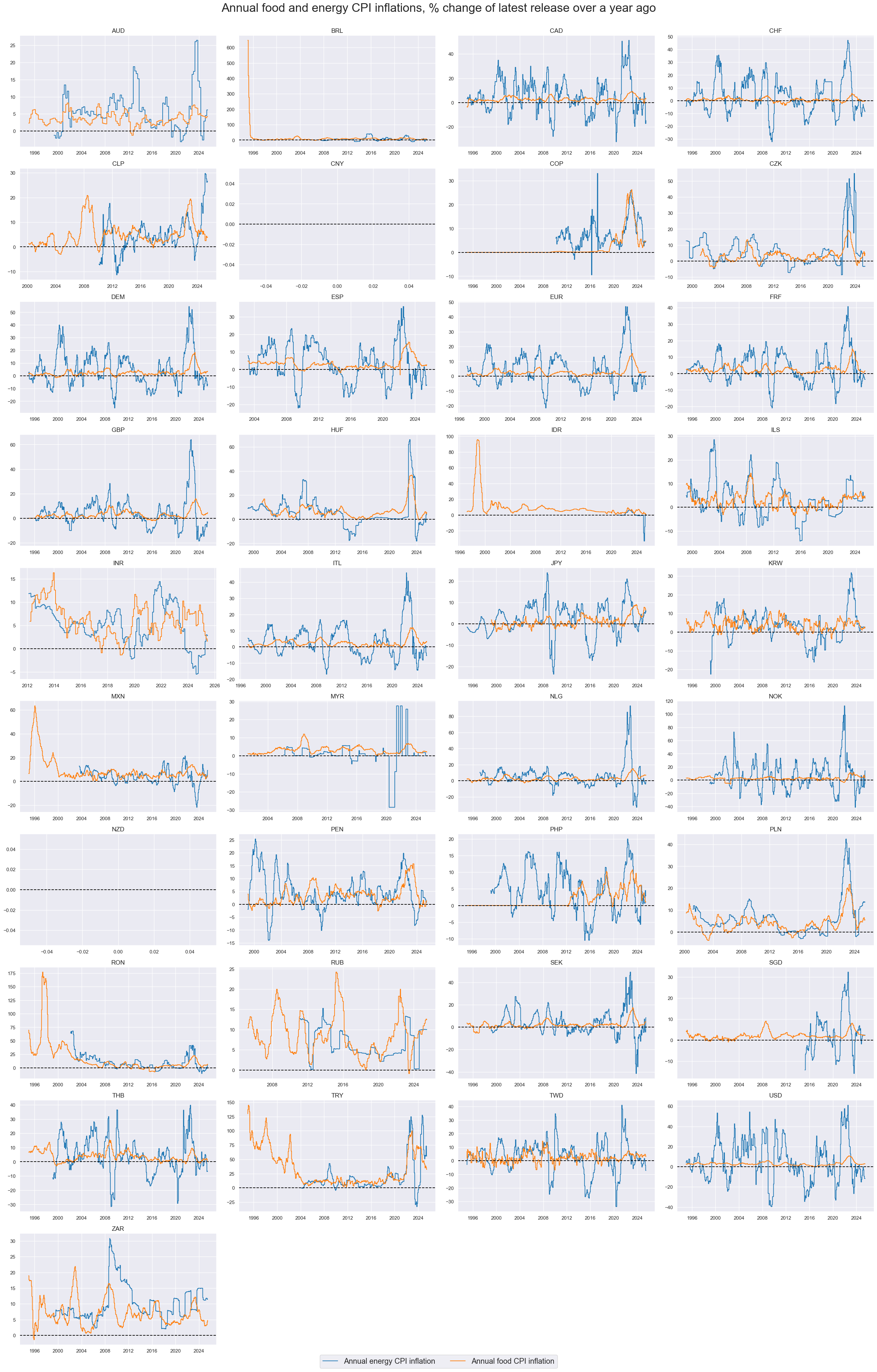
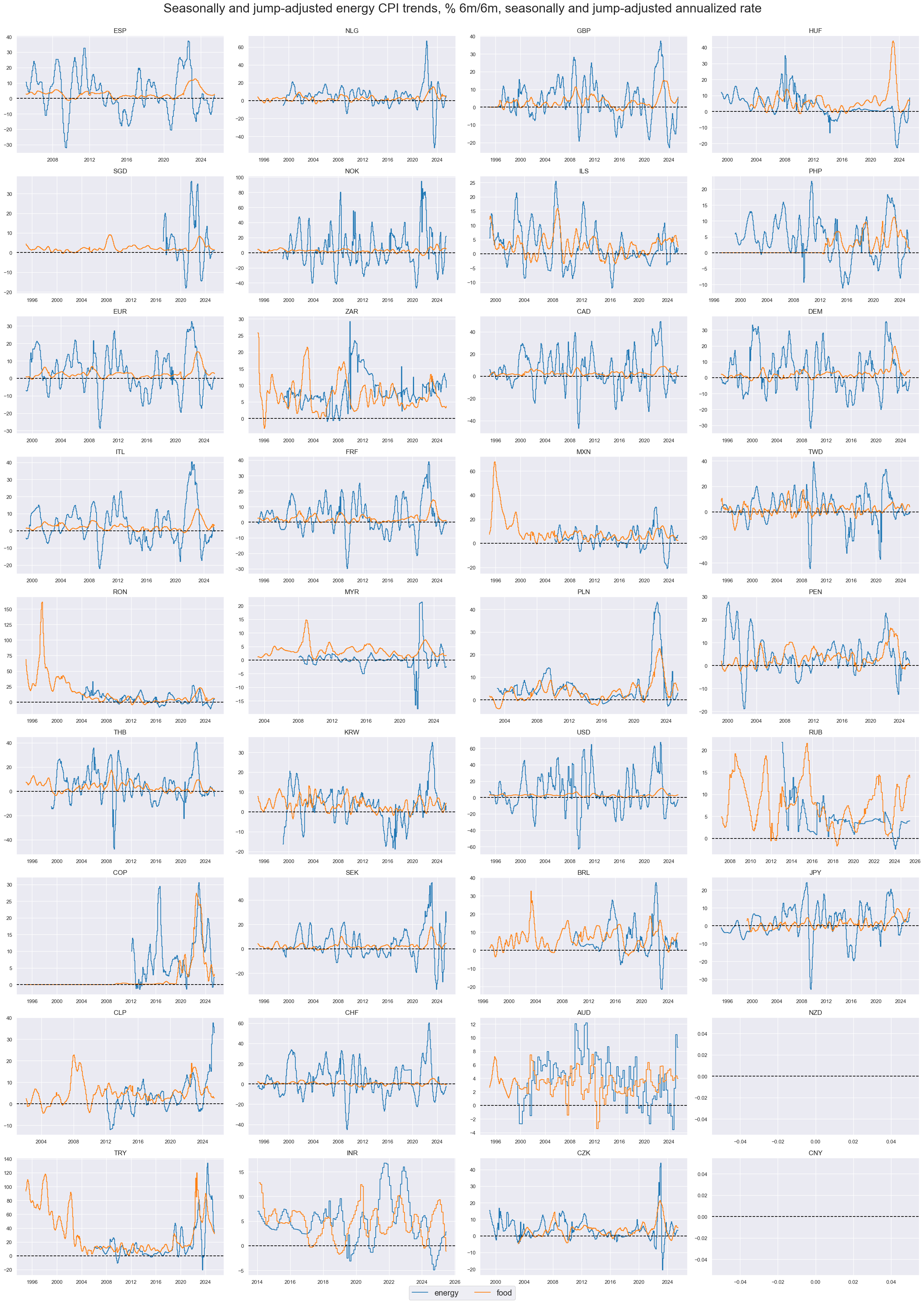
ALthough both category are volatile, energy price inflation tends to show much larger amplitudes.

xcatx = ["CPIE_SA_P1M1ML12", "CPIF_SA_P1M1ML12"]

msp.view_timelines(
    df,
    xcats=xcatx,
    cids=cids_exp,
    start=start_date,
    title="Annual food and energy CPI inflations, % change of latest release over a year ago",
    xcat_labels=[
        "Annual energy CPI inflation",
        "Annual food CPI inflation",
    ],
    legend_fontsize=17,
    title_fontsize=27,
    ncol=4,
    same_y=False,
    size=(16, 8),
    all_xticks=True,
)

Shoter-term adjusted food and energy CPI trends

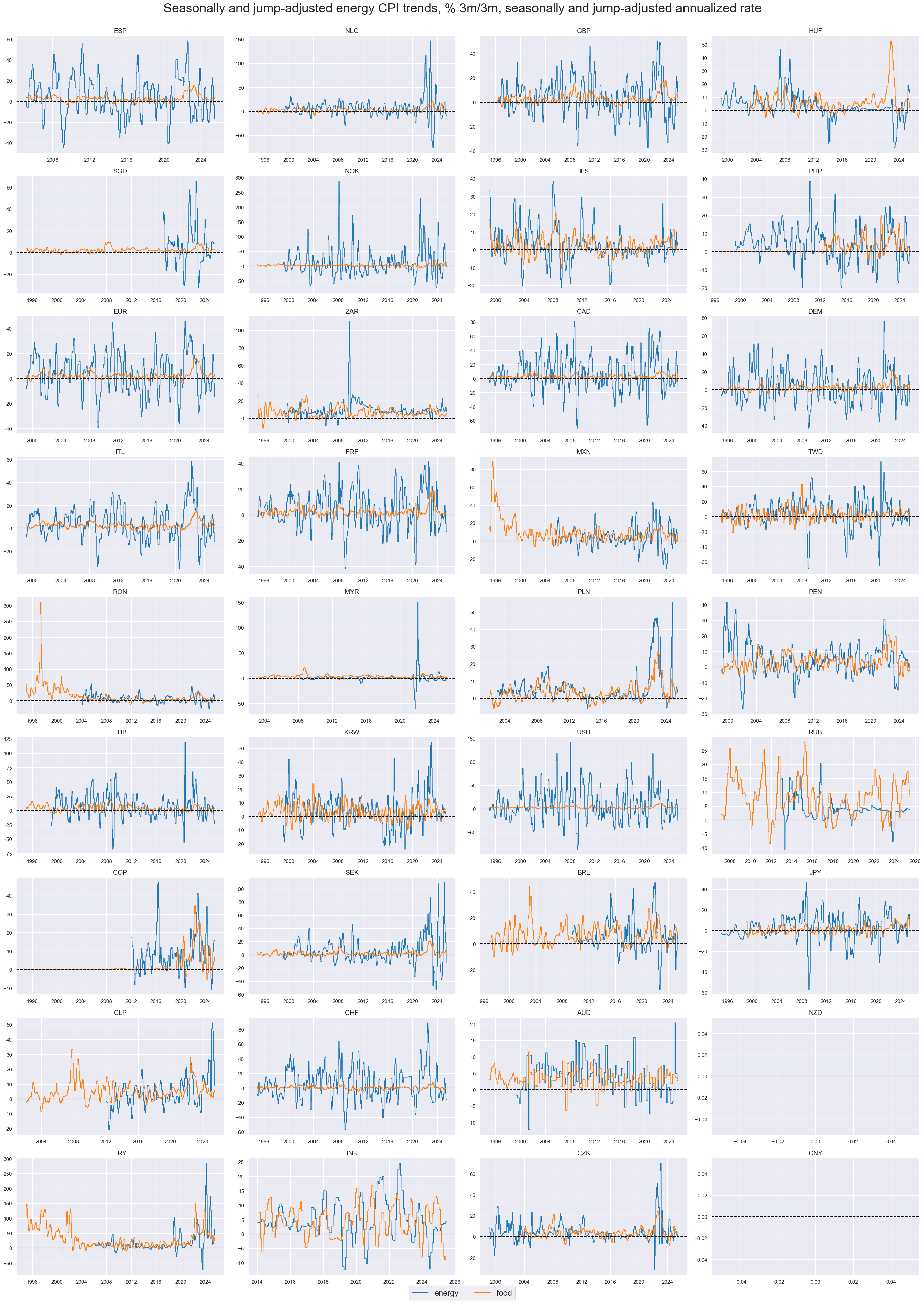
Fluctuations in short-term energy an food price growth are large, compared to other CPI areas. These fluctuations overshadow all medium-term trends.

xcatx = ["CPIE_SJA_P3M3ML3AR", "CPIF_SJA_P3M3ML3AR"]

msp.view_timelines(
    df,
    xcats=xcatx,
    cids=list(set(cids_exp) - set(["IDR"])),
    start=start_date,
    title="Seasonally and jump-adjusted energy CPI trends, % 3m/3m, seasonally and jump-adjusted annualized rate",
    xcat_labels=[
        "energy",
        "food",
    ],
    legend_fontsize=17,
    title_fontsize=27,
    ncol=4,
    same_y=False,
    all_xticks=True,
)

xcatx = ["CPIE_SJA_P6M6ML6AR", "CPIF_SJA_P6M6ML6AR"]

msp.view_timelines(
    df,
    xcats=xcatx,
    cids=list(set(cids_exp) - set(["IDR"])),
    start=start_date,
    title="Seasonally and jump-adjusted energy CPI trends, % 6m/6m, seasonally and jump-adjusted annualized rate",
    xcat_labels=[
        "energy",
        "food",
    ],
    legend_fontsize=17,
    title_fontsize=27,
    ncol=4,
    same_y=False,
    all_xticks=True,
)

Importance

Research links

Consistent core CPI trends rely on standardized indicators of core consumer price movements, making the research sources cited in the Consumer price inflation trends notebook applicable to this analysis as well. In addition, below are selected links on the significance of core inflation indicators and the challenges associated with comparing these indicators across different countries:

On the methodological differences of inflation measurements:

The term ‘core inflation’ is widely used by academics, central bankers and economic commentators. But despite its prevalence, there is neither a widely accepted theoretical definition nor an agreed method of measuring it. This may make it difficult to get a clear message from the measures, particularly when they have different trends. Bank of England WP 242

“Measuring inflation is a difficult but crucial task for national statistical agencies and doing so raises a host of methodological choices—and challenges. While advanced countries address many of these hurdles in similar ways, it is little surprise that methodological differences both large and small have also arisen over time.” The White House

“Economists and policymakers often track “core” inflation—inflation excluding volatile food and energy prices—because it tends to be a better predictor of future overall inflation than current “headline” inflation itself. But the precise definition of “core” varies by country. In the U.S., core CPI excludes both food at home (groceries) and food away from home (restaurants), while Japan only excludes “fresh food” from its core CPI (essentially groceries). Likewise, in Europe, the Eurostat measure core HICP only excludes “unprocessed foods” (also essentially groceries), but, confusingly, the core measure used by the European Central Bank excludes both groceries and restaurant food prices as well as alcohol and tobacco. These different definitions further obscure international comparisons.” The White House

“Two recent papers contribute to forecasting inflation in a world of convergent policy regimes and integrated economies. The first emphasizes the distinct effects of shocks to aggregate demand, supply, and monetary policy. The second explains why country inflation usually corrects deviations from trends in the rest of the world. Predominantly inflation has become a global force.” Macrosynergy

On the reasons for core inflation focus:

“The main reason to focus on the behavior of a core price measure is the belief that there is a significant amount of transitory noise in the movement of aggregate consumer prices.” Federal Reserve Bank of New York

“… the failure to detect the onset of inflationary pressures may lead to a sustained rise in inflation and ultimately require a more prolonged period of policy tightening. Then again, an overreaction to a temporary increase in inflation may result in an unwarranted slowing, and possible decline, in economic activity. Thus, the ability of central banks to differentiate between permanent and transitory price movements is critical for determining the appropriate prescription for monetary policy.” Federal Reserve Bank of New York

“When analysing inflation developments, it is important to distinguish between permanent changes and transitory changes in the level of prices. The behaviour of the Consumer Price Index (CPI) is affected by a range of erratic or transitory factors, which do not reflect fundamental changes to the behaviour of inflation determinants.” Bank of Portugal

Consistent core CPI trend indicators are used for example in the following Macrosyndergy posts:

• Excess inflation and asset class returns

Empirical clues

The empirical evidence supporting consistent core CPI trends aligns closely with the analyses conducted in the Consumer price inflation trends . However, the key distinction in this context is the emphasis on relative trades, both for developed and emerging markets. This focus sheds light on how inflation trends, when measured through a consistent core CPI lens, reveal distinct patterns and insights particularly relevant for understanding economic dynamics in developed and emerging economies with very specific methodology of calculating local inflation trends.

The focus in this notebook will be on:

• predictive power of relative consistent core CPI trends for directional and relative government bond returns,

• predictive power of relative consistent core CPI trends for relative duration returns,

• predictive power of relative consistent core CPI trends for relative fx returns.

scols = ["cid", "xcat", "real_date", "value"]
dfx = df[scols].copy().sort_values(["cid", "xcat", "real_date"])
dfx["ticker"] = dfx["cid"] + "_" + dfx["xcat"]

# The first step is to calculate the effective inflation target for each country. This is done by taking the maximum of the inflation target and 2%.


dfa = msp.panel_calculator(
    dfx, ["INFTEBASIS = INFTEFF_NSA.clip(lower=2)"], cids=cids
)  # `INFTEBASIS` is the maximum of the effective inflation target and 2.
dfx = msm.update_df(dfx, dfa)

#  for the primary Eurozone currencies duplicate the EUR values and assign them to their respective currencies.


xcatx = [
    "CPIXFE_SA_P1M1ML12",
    "CPIXFE_SJA_P6M6ML6AR",
    "CPIXFE_SA_P1M1ML12_D1M1ML3",
    "CPIC_SJA_P6M6ML6AR",
    "CPIC_SA_P1M1ML12",
    "INFTEFF_NSA",
    "INFTEBASIS",
]

calcs = [f"{xc}=  iEUR_{xc} + GB05YR_NSA - GB05YR_NSA" for xc in xcatx]

dfa = msp.panel_calculator(dfx, calcs=calcs, cids=cids_dmec)
dfx = msm.update_df(dfx, dfa)


# The last step is to calculate the relative deviations of the inflation rate from the effective inflation target.

sigx = [
    "CPIXFE_SA_P1M1ML12",
    "CPIXFE_SJA_P6M6ML6AR",
    "CPIC_SJA_P6M6ML6AR",
    "CPIC_SA_P1M1ML12",
    
]


for inf in sigx:
    calcs = [
        f"{inf}vIET = ( {inf} - INFTEFF_NSA ) / INFTEBASIS",
    ]
    dfa = msp.panel_calculator(dfx, calcs=calcs, cids=cids + cids_dmec)
    dfx = msm.update_df(dfx, dfa)

The analysis below focuses on FX and IRS receiver returns on vol-targeted positions. Before running the analysis, we use make_blacklist() helper function from macrosynergy package, which creates a standardized dictionary of blacklist periods, i.e. periods that affect the validity of an indicator, based on standardized panels of binary categories. As the next step, we take out bad data return periods for fixed-income markets for TRY

dfb = df[df["xcat"].isin(["FXTARGETED_NSA", "FXUNTRADABLE_NSA"])].loc[
    :, ["cid", "xcat", "real_date", "value"]
]
dfba = (
    dfb.groupby(["cid", "real_date"])
    .aggregate(value=pd.NamedAgg(column="value", aggfunc="max"))
    .reset_index()
)
dfba["xcat"] = "FXBLACK"
fxblack = msp.make_blacklist(dfba, "FXBLACK")

# we take out bad-data return periods for fixed income markets
filt_try = (dfx["cid"] == "TRY") & (dfx["real_date"] > pd.to_datetime("2022-08-01"))
dfx.loc[filt_try, "value"] = np.nan

Inflation and directional government bond returns

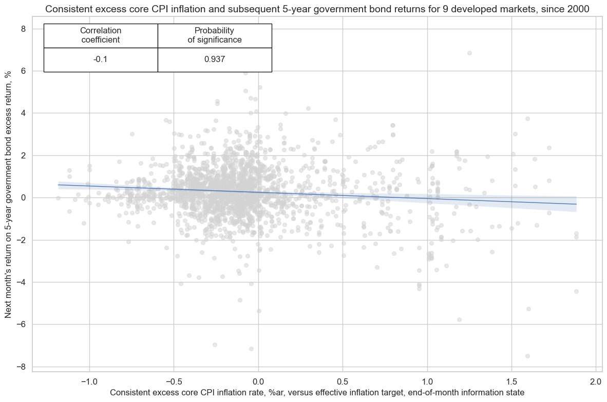
Core CPI inflation, or PCE inflation for the U.S., are key references for medium-term price stability and, hence, condition the stance of monetary policy in developed economies. Hence, tracking their trends consistently and carefully relative to effective inflation targets is a valid basis for predicting trends in the rates market. This reflects rational inattention of a large share of investors. Excess inflation should systematically annd negatively predict high-grade bond returns under this assumption. In the notebook “Consumer price inflation trends” this relationship is shown for the US. However, using consistent inflation data, one can do a similar analysis for all developed markets (‘AUD’, ‘DEM’, ‘ESP’, ‘FRF’, ‘GBP’, ‘ITL’, ‘JPY’, ‘NZD’, ‘USD’) collected in the list cids_bond . Indeed, the relation between excess core inflation and subsequent 5-year IRS bond returns has been negative and significantly so, according to the Macrosynergy panel test, at weekly, monthly, and quarterly frequencies.

cr_bond_consist = msp.CategoryRelations(
    dfx,
    xcats=["CPIXFE_SJA_P6M6ML6ARvIET", "GB05YR_NSA"],
    cids=cids_bond,
    freq="M",
    lag=1,
    blacklist=fxblack,
    xcat_aggs=["last", "sum"],
    start="2000-01-01",
)

cr_bond_consist.reg_scatter(
    title="Consistent excess core CPI inflation and subsequent 5-year government bond returns for 9 developed markets, since 2000",
    labels=False,
    coef_box="upper left",
    xlab="Consistent excess core CPI inflation rate, %ar, versus effective inflation target, end-of-month information state",
    ylab="Next month's return on 5-year government bond excess return, %",
    prob_est="map"
)

Inflation and relative government bond returns

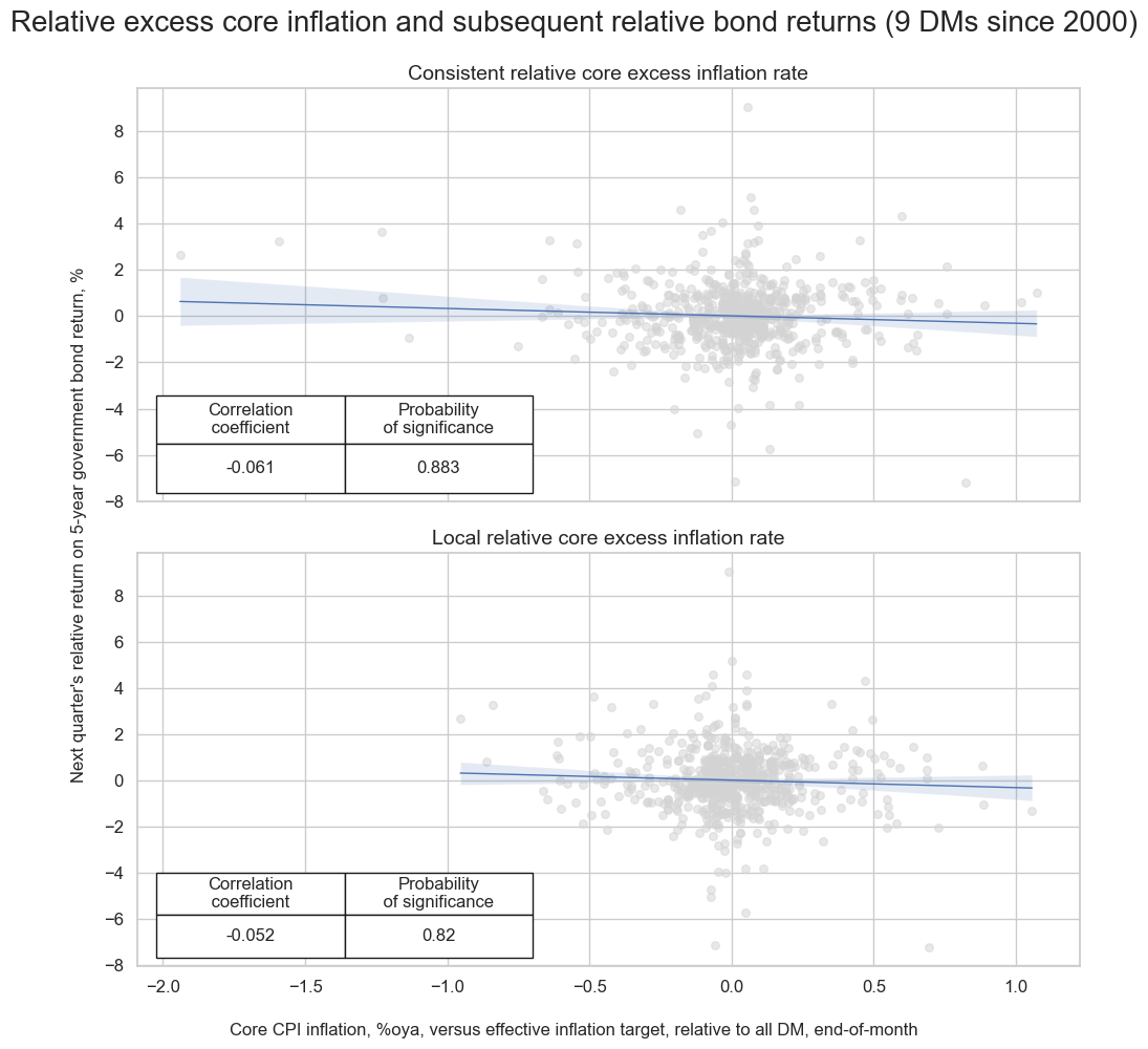
Consistent core inflation is particularly useful for tracking relative inflation pressure. Indeed, relative consistent core CPI trends have negatively predicted relative 5-year government bond returns in the past with modest signficance and, hence, a promising basis for cross-market duration allocations or relative value trends. The negative predictive correlation between relative core inflation and relative government bond returns has been stronger if one uses consistent inflation metrics instead of those based on local conventions.

dfa = msp.make_relative_value(
    dfx,
    xcats=["GB05YR_NSA", "CPIXFE_SA_P1M1ML12vIET", "CPIC_SA_P1M1ML12vIET"],
    cids=cids_bond,
    postfix="vDM",
)
dfx = msm.update_df(dfx, dfa)

cr_relbond_consist = msp.CategoryRelations(
    dfx,
    xcats=["CPIXFE_SA_P1M1ML12vIETvDM", "GB05YR_NSAvDM"],
    cids=cids_bond,
    freq="Q",
    lag=1,
    xcat_aggs=["last", "sum"],
    start="2000-01-01",
)

cr_relbond_local = msp.CategoryRelations(
    dfx,
    xcats=["CPIC_SA_P1M1ML12vIETvDM", "GB05YR_NSAvDM"],
    cids=cids_bond,
    freq="Q",
    lag=1,
    xcat_aggs=["last", "sum"],
    start="2000-01-01",
)

msv.multiple_reg_scatter(
        [cr_relbond_consist, cr_relbond_local],
        title="Relative excess core inflation and subsequent relative bond returns (9 DMs since 2000)",
        xlab="Core CPI inflation, %oya, versus effective inflation target, relative to all DM, end-of-month",
        ylab="Next quarter's relative return on 5-year government bond return, %",
        ncol=1,
        nrow=2,
        figsize=(10, 10),
        prob_est="map",
        coef_box="lower left", 
        subplot_titles=["Consistent relative core excess inflation rate", "Local relative core excess inflation rate"],
     )

Relative consistent core inflation as a predictor of relative IRS returns

Here, we define relative consistent core inflation as the %oya, %6m/6m, saar, %3m/3m, saar excess inflation rate of one currency area versus the average of basket of currencies. We define two relative inflation metrics:

• versus basket of developed markets ( vDM ), and

• versus basket of all available markets ( vGM ).

dfa = msp.make_relative_value(
    dfx,
    xcats=[
        "DU02YXR_VT10",
        "DU05YXR_VT10",
        "CPIXFE_SA_P1M1ML12vIET",
        "CPIXFE_SJA_P6M6ML6ARvIET",
    ],
    cids=cids_dmca,
    postfix="vDM",
)
dfx = msm.update_df(dfx, dfa)

dfa = msp.make_relative_value(
    dfx,
    xcats=[
        "DU02YXR_VT10",
        "DU05YXR_VT10",
        "CPIXFE_SA_P1M1ML12vIET",
        "CPIXFE_SJA_P6M6ML6ARvIET",
   ],
    cids=cids_irs,
    postfix="vGM",
)
dfx = msm.update_df(dfx, dfa)

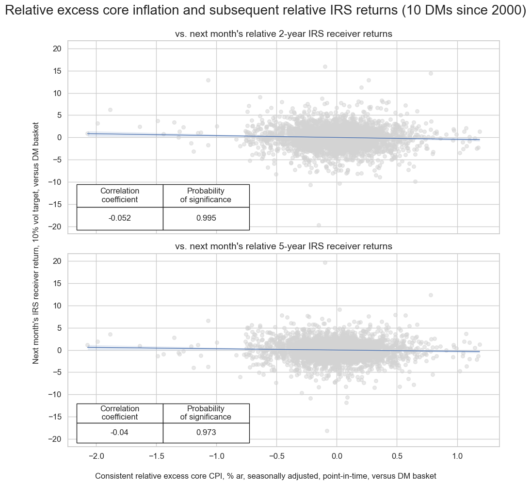
Relative excess consistent core inflation rates in the developed markets (one country versus all others) have negatively predicted relative IRS fixed receiver returns, across various maturities. This supports the hypothesis that core inflation performance is guide for cross-currency duration and relative cross-currency duration trades. The predictive power is stronger for shorter maturities than for longer maturities.

crvDM_IRS2 = msp.CategoryRelations(
    dfx,
    xcats=["CPIXFE_SA_P1M1ML12vIETvDM", "DU02YXR_VT10vDM"],
    cids=cids_dmca,
    freq="M",
    lag=1,
    xcat_aggs=["last", "sum"],
    blacklist=fxblack,
    start="2000-01-01",
    xcat_trims=[20, 20],
)
crvDM_IRS5 = msp.CategoryRelations(
    dfx,
    xcats=["CPIXFE_SA_P1M1ML12vIETvDM", "DU05YXR_VT10vDM"],
    cids=cids_dmca,
    freq="M",
    lag=1,
    xcat_aggs=["last", "sum"],
    blacklist=fxblack,
    start="2000-01-01",
    xcat_trims=[20, 20],
)

msv.multiple_reg_scatter(
        [crvDM_IRS2, crvDM_IRS5],
        title="Relative excess core inflation and subsequent relative IRS returns (10 DMs since 2000)",
        xlab="Consistent relative excess core CPI, % ar, seasonally adjusted, point-in-time, versus DM basket",
        ylab="Next month's IRS receiver return, 10% vol target, versus DM basket",
        ncol=1,
        nrow=2,
        figsize=(10, 10),
        prob_est="map",
        coef_box="lower left", 
        subplot_titles=["vs. next month's relative 2-year IRS receiver returns", 
        "vs. next month's relative 5-year IRS receiver returns"],
)

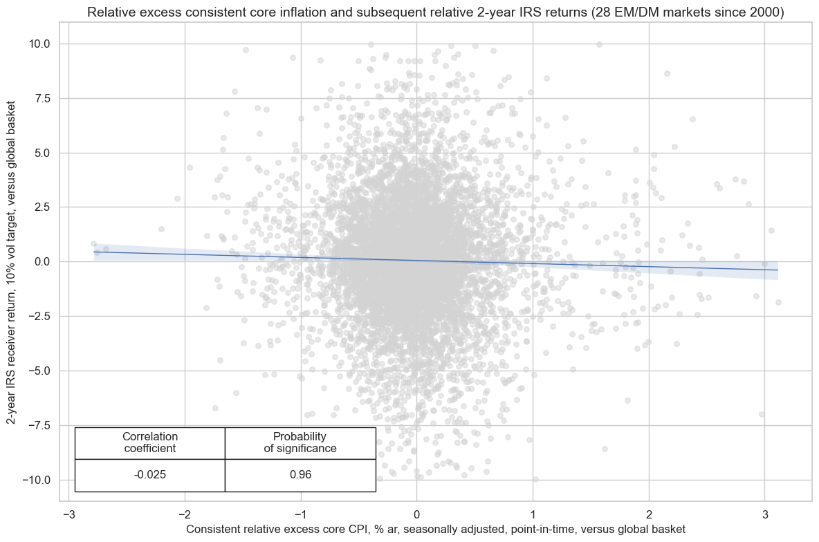
The negative predictive power of relative excess consistent core inflation rates is weaker for a global set of DM and EM countries than for the developed markets alone. This illustrates that core inflation is not an accepted standard everywhere and that without further adjustment inflation excesses or shortfalls are not easily comparable across economies with different structures and policy regimes.

xcatx=["CPIXFE_SA_P1M1ML12vIETvGM", "DU02YXR_VT10vGM"]

crvGM_IRS2 = msp.CategoryRelations(
    dfx,
    xcats=xcatx,
    cids=cids_irs,
    freq="M",
    blacklist=fxblack,
    lag=1,
    xcat_aggs=["last", "sum"],
    start="2000-01-01",
    xcat_trims=[10, 10],
)

crvGM_IRS2.reg_scatter(
    labels=False,
    coef_box="lower left",
    title="Relative excess consistent core inflation and subsequent relative 2-year IRS returns (28 EM/DM markets since 2000)",    
    xlab="Consistent relative excess core CPI, % ar, seasonally adjusted, point-in-time, versus global basket",
    ylab="2-year IRS receiver return, 10% vol target, versus global basket",
    size=(12, 8),
    prob_est="map",
)

Excess inflation ratios versus FX benchmarks

The inflation aversion of central banaks in developed countries implies that higher sustained inflation pressure typically invites tighter policies, in actions and words.

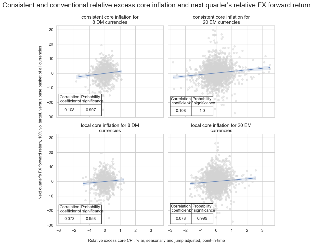
There has been a strong relation between excess inflation, against base currency and a basket of currencies, and FX forward returns, again against base and against a basket of currencies. This predictive relation is valuable because it allows creating a more diversified FX portfolio and reduces the dominant influence of dollar and euro against all other currencies.

cids_eur = ["CHF", "CZK", "HUF", "NOK", "PLN", "RON", "SEK"]  # trading against EUR
cids_eud = ["GBP", "RUB", "TRY"]  # trading against EUR and USD
cids_usd = list(set(cids_fx) - set(cids_eur + cids_eud))  # trading against USD


xcatx = ["CPIXFE_SA_P1M1ML12vIET", "CPIXFE_SJA_P6M6ML6ARvIET", "CPIC_SJA_P6M6ML6ARvIET"]

for xc in xcatx:
    calc_eur = [f"{xc}vBM = {xc} - iEUR_{xc}"]
    calc_usd = [f"{xc}vBM = {xc} - iUSD_{xc}"]
    calc_eud = [f"{xc}vBM = {xc} - 0.5 * ( iEUR_{xc} + iUSD_{xc} )"]

    dfa_eur = msp.panel_calculator(
        dfx,
        calcs=calc_eur,
        cids=cids_eur,
    )
    dfa_usd = msp.panel_calculator(
        dfx,
        calcs=calc_usd,
        cids=cids_usd,
    )
    dfa_eud = msp.panel_calculator(
        dfx,
        calcs=calc_eud,
        cids=cids_eud,
    )

    dfa = pd.concat([dfa_eur, dfa_usd, dfa_eud])
    dfx = msm.update_df(dfx, dfa)

dfa = msp.make_relative_value(
    dfx,
    xcats=["CPIXFE_SJA_P6M6ML6ARvIETvBM", "FXXR_VT10", "CPIC_SJA_P6M6ML6ARvIETvBM"],
    cids=cids_dmfx,
    postfix="vDM",
)

dfx = msm.update_df(dfx, dfa)


dfa = msp.make_relative_value(
    dfx,
    xcats=["CPIXFE_SJA_P6M6ML6ARvIETvBM", "FXXR_VT10", "CPIC_SJA_P6M6ML6ARvIETvBM"],
    cids=cids_fx,
    postfix="vGFX",
)

dfx = msm.update_df(dfx, dfa)

The relationship known as the “double relative” applies to both developed and emerging markets, becoming more pronounced when using consistent inflation measures.

crxvBMvDM_fx = msp.CategoryRelations(
    dfx,
    xcats=["CPIXFE_SJA_P6M6ML6ARvIETvBMvDM", "FXXR_VT10vDM"],
    cids=cids_dmfx,
    freq="Q",
    lag=1,
    xcat_aggs=["last", "sum"],
    blacklist=fxblack,
    start="2000-01-01",
    xcat_trims=[10, 30],
)

crxvBMvGM_fx = msp.CategoryRelations(
    dfx,
    xcats=["CPIXFE_SJA_P6M6ML6ARvIETvBMvGFX", "FXXR_VT10vGFX"],
    cids=cids_emfx,
    freq="Q",
    lag=1,
    xcat_aggs=["last", "sum"],
    blacklist=fxblack,
    start="2000-01-01",
    xcat_trims=[10, 30],
)

crxvBMvDM_fx_local = msp.CategoryRelations(
    dfx,
    xcats=["CPIC_SJA_P6M6ML6ARvIETvBMvDM", "FXXR_VT10vDM"],
    cids=cids_dmfx,
    freq="Q",
    lag=1,
    xcat_aggs=["last", "sum"],
    blacklist=fxblack,
    start="2000-01-01",
    xcat_trims=[10, 30],
)

crxvBMvGM_fx_local = msp.CategoryRelations(
    dfx,
    xcats=["CPIC_SJA_P6M6ML6ARvIETvBMvGFX", "FXXR_VT10vGFX"],
    cids=cids_emfx,
    freq="Q",
    lag=1,
    xcat_aggs=["last", "sum"],
    blacklist=fxblack,
    start="2000-01-01",
    xcat_trims=[10, 30],
)

msv.multiple_reg_scatter(
        [crxvBMvDM_fx, crxvBMvGM_fx, crxvBMvDM_fx_local, crxvBMvGM_fx_local],
        title="Consistent and conventional relative excess core inflation and next quarter's relative FX forward return",
        xlab="Relative excess core CPI, % ar, seasonally and jump adjusted, point-in-time",
        ylab="Next quarter's FX forward return, 10% vol target, versus base basket of all currencies",
        figsize=(10, 10),
        nrow=2,
        ncol=2,
        prob_est="map",
        coef_box="lower left", 
        subplot_titles=["consistent core inflation for 8 DM currencies", 
        "consistent core inflation for 20 EM currencies", "local core inflation for 8 DM currencies",
        "local core inflation for 20 EM currencies", 
        ],
)

naive_pnl_dmfx = msn.NaivePnL(
    dfx,
    ret="FXXR_VT10vDM",
    sigs=["CPIXFE_SJA_P6M6ML6ARvIETvBMvDM"],
    cids=cids_dmfx,
    start="2000-01-01",
 
)

naive_pnl_dmfx.make_pnl(
    sig = "CPIXFE_SJA_P6M6ML6ARvIETvBMvDM",
    sig_neg=False,
    sig_op="zn_score_pan",
    thresh=3,
    rebal_freq="monthly",
    vol_scale=10,
    rebal_slip=1,
 
)

naive_pnl_dmfx.make_long_pnl(vol_scale=10, label="Long")

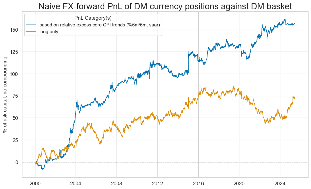
We estimate the economic value of related strategies based on a standard naïve PnL methodology used in many previous research posts. This PnL is calculated for simple monthly rebalancing in accordance with the relative core inflation score, normalized, and winsorized at three standard deviations at the end of each month. The end-of-month score is the basis for the positions of the next month under the assumption of a 1-day slippage for trading. The naïve PnL does not consider transaction costs or compounding. For the chart below, the PnL has been scaled to an annualized volatility of 10%.

Since the relative excess core inflation signal produces 8 diversified and principally non-directional trades each month, it creates a strong long-term PnL performance prior to transaction costs.

naive_pnl_dmfx.plot_pnls(
    pnl_cats=naive_pnl_dmfx.pnl_names,
    pnl_cids=["ALL"],
    title="Naive FX-forward PnL of DM currency positions against DM basket",
    xcat_labels=["based on relative excess core CPI trends (%6m/6m, saar)",
                 "long only"]
    )

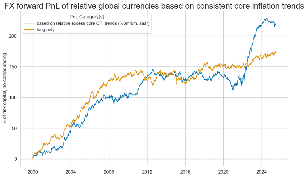
Before accounting for transaction costs, the long-term profit and loss performance is significantly better in emerging markets, albeit also more seasonal.

naive_pnl_gfx = msn.NaivePnL(
    dfx,
    ret="FXXR_VT10vGFX",
    sigs=["CPIXFE_SJA_P6M6ML6ARvIETvBMvGFX"],
    cids=cids_emfx,
    start="2000-01-01",
)

naive_pnl_gfx.make_pnl(
    sig = "CPIXFE_SJA_P6M6ML6ARvIETvBMvGFX",
    sig_neg=False,
    sig_op="zn_score_pan",
    thresh=3,
    rebal_freq="monthly",
    vol_scale=10,
    rebal_slip=1,
 
)

naive_pnl_gfx.make_long_pnl(vol_scale=10, label="Long")

naive_pnl_gfx.plot_pnls(
    pnl_cats=naive_pnl_gfx.pnl_names,
    pnl_cids=["ALL"],
    title="FX forward PnL of relative global currencies based on consistent core inflation trends",
    xcat_labels=["based on relative excess core CPI trends (%6m/6m, saar)", 
                 "long only"]
    )

Excess energy inflation and relative equity sector returns

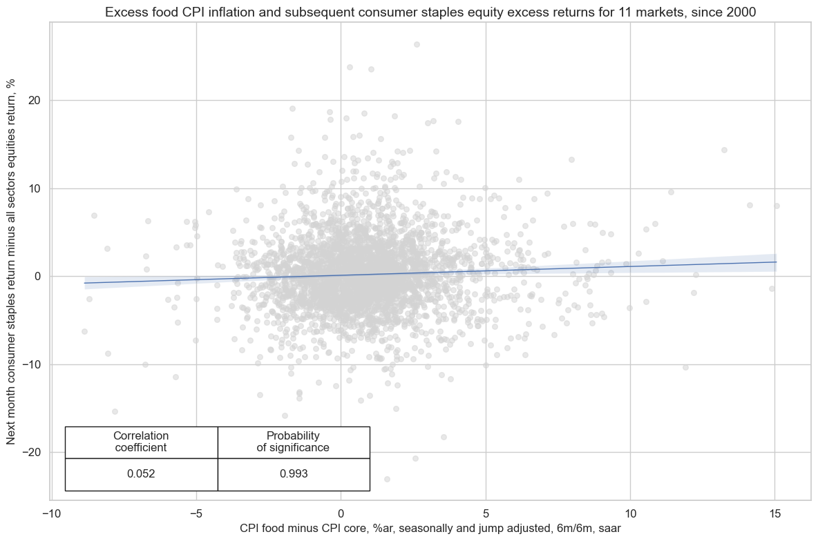
Food and energy CPI inflation plausibly heralds outperformance of the sectors that charge these volatile prices versus other sectors. In times of high food and energy inflation price markups are more likely in consumer staples and energy, while purchasing power is reduced in other sectors.

Indeed, since 2000 CPI food inflation has been a highly significant predictor of consumer staples sector returns versus the overall market, across developed countries and across time. The probability of significance has also been positive and significant in subsamples, testifying to robustness.

# Excess food and energy inflation
chgs = ["SA_P1M1ML12", "SJA_P3M3ML3AR", "SJA_P6M6ML6AR"]
cpis = ["CPIE", "CPIF"]

calcs = [f"X{cpi}_{chg} = {cpi}_{chg} - CPIXFE_{chg}" for chg in chgs for cpi in cpis]
dfa = msp.panel_calculator(dfx, calcs=calcs, cids=cids + cids_dmec)

dfx = msm.update_df(dfx, dfa)

# Excess enery and consumer staples returns
calcs = [
    f"EQC{sec}R_NSAvALL = EQC{sec}R_NSA - EQCALLR_NSA" for sec in ["ENR", "COS"]
]
dfa = msp.panel_calculator(dfx, calcs=calcs, cids=cids + cids_dmec)
dfx = msm.update_df(dfx, dfa)

xcatx = ["XCPIF_SJA_P6M6ML6AR", "EQCCOSR_NSAvALL"]
cidx = cids_eq

cr = msp.CategoryRelations(
    dfx,
    xcats=xcatx,
    freq="M",
    cids=cidx,
    blacklist=None,
    lag=1,
    xcat_aggs=["last", "sum"],
    start="2000-01-01",
)

cr.reg_scatter(
    labels=False,
    coef_box="lower left",
    title="Excess food CPI inflation and subsequent consumer staples equity excess returns for 11 markets, since 2000",
    xlab="CPI food minus CPI core, %ar, seasonally and jump adjusted, 6m/6m, saar",
    ylab="Next month consumer staples return minus all sectors equities return, %",
    size=(12, 8),
    prob_est="map",
)

XCPIF_SJA_P6M6ML6AR misses: ['NZD'].

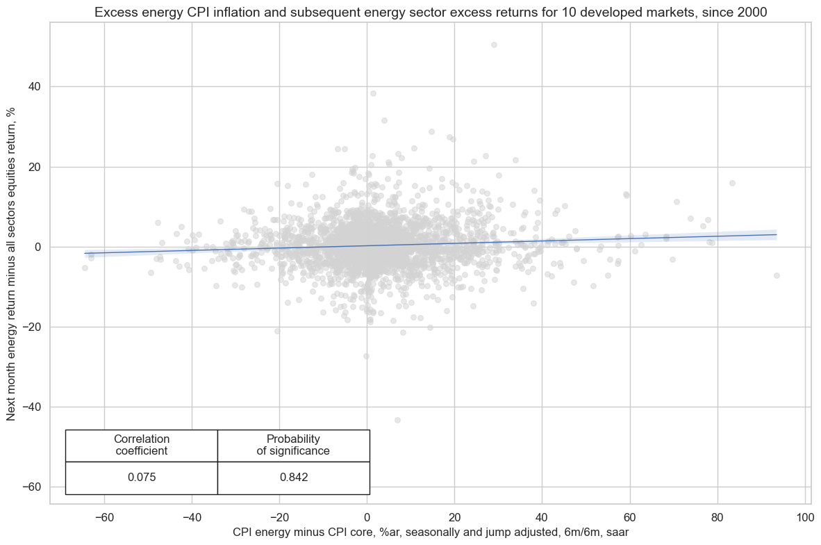
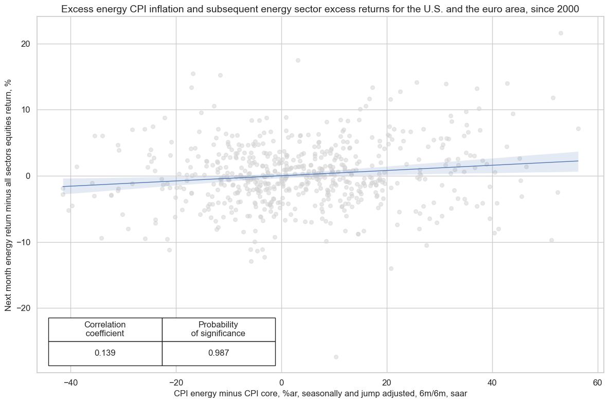
There is also evidence of positive predictive relation between energy CPI growth versus core CPI growth and subsequent energy sector relative returns versus the overall market. However, the relationship is only really significant for the large countries, as for small countries the home markets’ price developments are less important than global energy price trends.

xcatx = ["XCPIE_SJA_P6M6ML6AR", "EQCENRR_NSAvALL"]
cidx = cids_eq

cr = msp.CategoryRelations(
    dfx,
    xcats=xcatx,
    freq="M",
    cids=cidx,
    blacklist=None,
    lag=1,
    xcat_aggs=["last", "sum"],
    start="2000-01-01",
)

cr.reg_scatter(
    labels=False,
    coef_box="lower left",
    title="Excess energy CPI inflation and subsequent energy sector excess returns for 10 developed markets, since 2000",
    xlab="CPI energy minus CPI core, %ar, seasonally and jump adjusted, 6m/6m, saar",
    ylab="Next month energy return minus all sectors equities return, %",
    size=(12, 8),
    prob_est="map",
)

XCPIE_SJA_P6M6ML6AR misses: ['NZD'].
EQCENRR_NSAvALL misses: ['CHF'].

xcatx = ["XCPIE_SA_P1M1ML12", "EQCENRR_NSAvALL"]
cidx = ["EUR", "USD"]

cr = msp.CategoryRelations(
    dfx,
    xcats=xcatx,
    freq="M",
    cids=cidx,
    blacklist=None,
    lag=1,
    xcat_aggs=["last", "sum"],
    start="2000-01-01",
)

cr.reg_scatter(
    labels=False,
    coef_box="lower left",
    title="Excess energy CPI inflation and subsequent energy sector excess returns for the U.S. and the euro area, since 2000",
    xlab="CPI energy minus CPI core, %ar, seasonally and jump adjusted, 6m/6m, saar",
    ylab="Next month energy return minus all sectors equities return, %",
    size=(12, 8),
    prob_est="map",
)

Appendices

Appendix 1: Indicator calculations

First obtain the seasonally adjusted headline CPI series from the raw data. For some cross-sections the adjustment is performed in JPMaQS, whilst occasionally this is prevalent in the underlying raw data. Secondly, each non-core CPI component (and respective weights) are obtained from the raw data. Whilst these components may vary for different cross-sections, these are broadly:

• food and non-alcoholic beverages

• alcoholic beverages and tobacco

• energy

• fuel for personal transport

Next, the following two series’ are calculated:

• Headline CPI, seasonally-adjusted, 1-year % change

• Non-core CPI, seasonally-adjusted, 1-year % change

The non-core CPI series is proportional to a weighted sum of the 1-year % change in seasonally-adjusted non-core CPI component contributions.

Finally, the total sum of weights is calculated and the annual consistent core CPI is given by:

(1) \[\begin{equation} \text{Annual consistent core CPI} = 100 \times \text{cprod} \left(1+ \frac{\text{1 year \% change in headline CPI} - {\text{1 year \% change in non-core CPI}}}{1-\frac{1}{100}\times\text{Total weights}} \right) \end{equation}\]

Appendix 2: Currency symbols

The word ‘cross-section’ refers to currencies, currency areas or economic areas. In alphabetical order, these are AUD (Australian dollar), BRL (Brazilian real), CAD (Canadian dollar), CHF (Swiss franc), CLP (Chilean peso), CNY (Chinese yuan renminbi), COP (Colombian peso), CZK (Czech Republic koruna), DEM (German mark), ESP (Spanish peseta), EUR (Euro), FRF (French franc), GBP (British pound), HKD (Hong Kong dollar), HUF (Hungarian forint), INR (Indian rupee), IDR (Indonesian rupiah), ILS (Israeli shekel), ITL (Italian lira), JPY (Japanese yen), KRW (Korean won), MXN (Mexican peso), MYR (Malaysian ringgit), NLG (Dutch guilder), NOK (Norwegian krone), NZD (New Zealand dollar), PEN (Peruvian sol), PHP (Phillipine peso), PLN (Polish zloty), RON (Romanian leu), RUB (Russian ruble), SEK (Swedish krona), SGD (Singaporean dollar), THB (Thai baht), TRY (Turkish lira), TWD (Taiwanese dollar), USD (U.S. dollar), ZAR (South African rand).