Cross-country relative duration strategies with macro factors

Jupyter Notebook

Cross-country relative duration strategies take vol-adjusted fixed receiver positions in interest rate swaps of one currency area versus others. Similar to directional IRS strategies, cross-country trading factors can be based on point-in-time indicators of economic developments. The main difference is that cross-country factors are typically related to relative economic performance.
This post constructs 12 conceptual macro factors that theoretically should help predict cross-country vol-targeted duration returns. Empirically, all of them have displayed at least some modest predictive power, while their cross-correlations have been mostly modest and very diverse. Composite signals can be generated by conceptual parity or sequential machine learning methods. All of these have produced material, consistent, and uncorrelated risk-adjusted returns over the past two decades with few major drawdowns.

The post below is based on Macrosynergy’s proprietary research. Please quote as “Gholkar, Rushil and Sueppel, Ralph, ‘A cross-country relative duration strategy with macro factors,’ Macrosynergy research post, June 2025.”

A Jupyter notebook for audit and replication of the research results can be downloaded here. The notebook operation requires access to J.P. Morgan DataQuery to download data from JPMaQS. Everyone with DataQuery access can download data except for the latest months. Moreover, J.P. Morgan offers free trials on the complete dataset for institutional clients. An academic support program sponsors data sets for research projects.

The idea in a nutshell

A “plain vanilla” interest swap (IRS) is an over-the-counter derivative contract, which obligates one party to pay a fixed interest rate and the other to pay a variable interest rate based on an official benchmark. As no notional is exchanged, the contract carries little credit risk, except for some counterparty risk for the party that is “in the money”. Therefore, the fixed receiver leg in an IRS is suitable for taking pure duration exposure, i.e., a position that pays a profit if future long-term yields decline and incurs a loss when they rise with little influence of the credit risk of a particular issuer.

Previous research has shown that point-in-time macroeconomic factors are predictors of directional duration returns, both theoretically and empirically. Predictive directional macro factors include information state changes in economic growth, economic sentiment, labor market conditions, inflation, and financial conditions (view post) as well as information states of excess aggregate demand in the economy (view post), merchandise import growth (view post), and real long-term yields based on formulaic inflation expectations (view post). Markets fail to fully price all these economic developments due to rational inattention (view post).

Generally, returns on duration positions are positively correlated across countries and, in most cases, strongly so. The below 5-year IRS return correlation matrix for 24 developed and emerging market currency areas since 2000 shows that almost all country pairs have displayed positive correlation at a monthly frequency. Most Pearson correlation coefficients have been in a range of 30-70%, and some country pairs, such as the U.S. and Canada or the euro area and its neighbours, reached 80%. This reflects that the PnLs of directional rates trading strategies are dominated by global trends or developments in the large, developed economies.

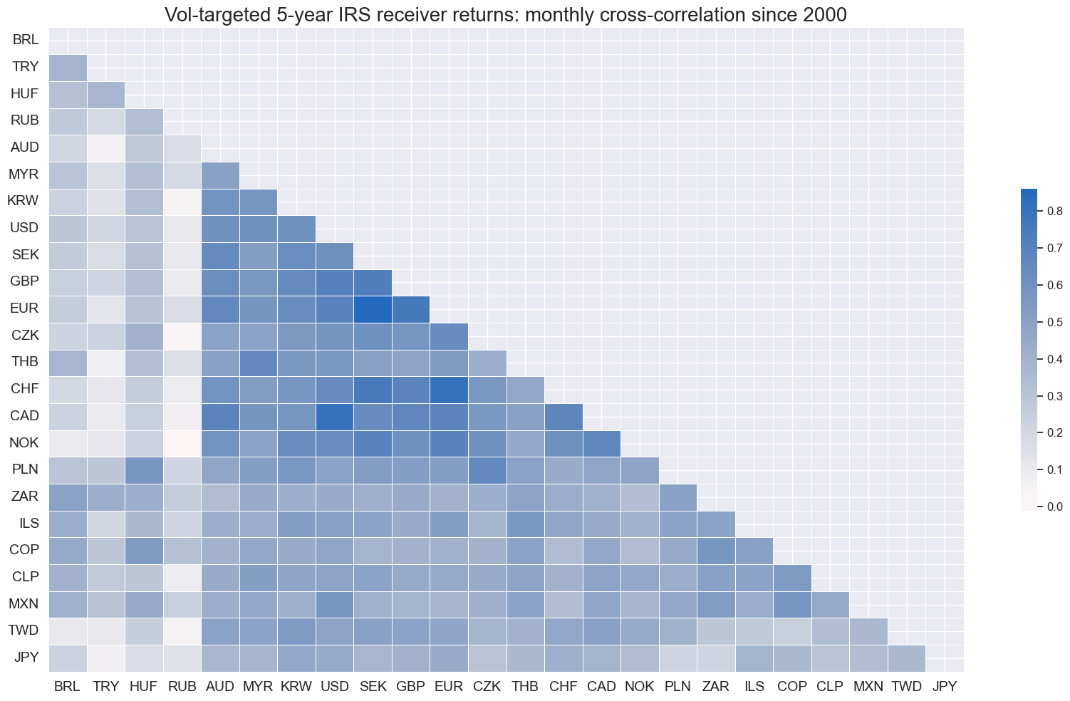
This means that complementary returns can be generated by focusing on cross-country relative duration exposure. Here we define such exposure as positions with a 10% volatility target in one currency area versus a basket of volatility-targeted positions in all concurrently tradable currency areas, whereby the target for each constituent is 10% divided by the number of constituents. The volatility targeting is necessary to make risk exposure comparable across developed and emerging countries.

The central hypothesis is that returns on relative duration positions can be predicted using macroeconomic factors that capture cross-country divergences, such as differences in growth, inflation, or trade-weighted exchange rate changes. We identify a range of these divergence factors below and combine them into unified trading signals using either the principle of conceptual parity or sequential machine learning.

Cross-country IRS returns since 2000

For this post, we consider IRS markets in 24 currency areas, of which nine are classified as developed markets and 15 as emerging markets. These are almost all markets that, since 2000, have provided at least temporarily good liquidity in the local rates market as well as a flexible exchange rate. Countries and periods with pegged exchange rates have been disregarded due to the dependence of the monetary policy on conditions in the pegged currency area. Countries whose markets have “blown up” and become temporarily untradable, such as Russia and Turkey, are included to make the backtests more realistic.

• The developed market currency areas are (in alphabetical order if the currency symbol): Australia (AUD), Canada (CAD), Switzerland (CHF), the euro area (EUR), the United Kingdom (GBP), Japan (JPY), Norway (NOK), Sweden (SEK), and the United States (USD).
• The emerging markets are Brazil (BRL), Chile (CLP), Colombia (COP), Czechia (CZK), Hungary (HUF), Israel (ILS), South Korea (KRW), Mexico (MXN), Malaysia (MYR), Poland (PLN), Russia (RUB), Thailand (THB), Turkey (TRY), Taiwan (TWD), and South Africa (ZAR).

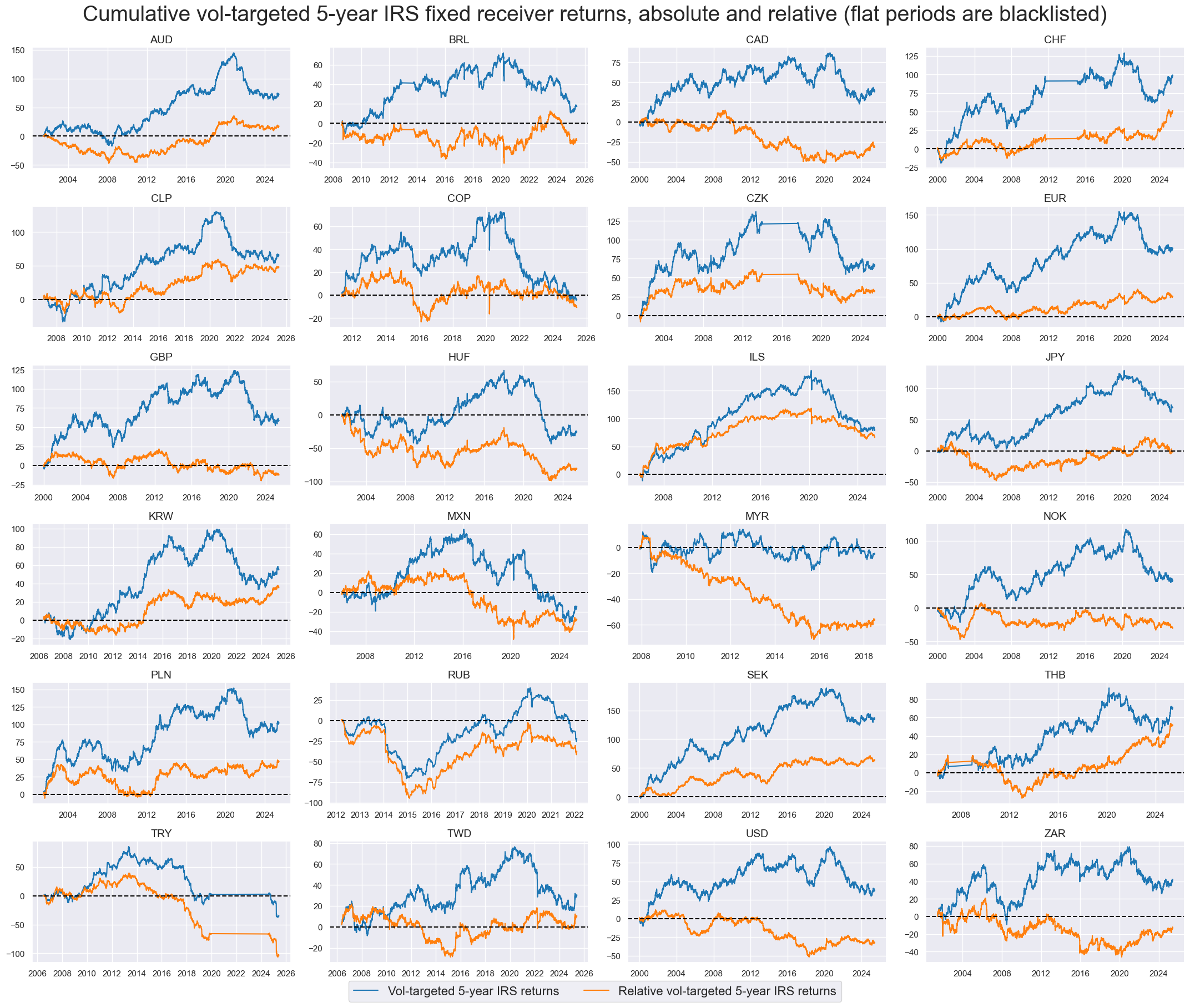
Generic returns on vol-targeted positions have been taken from the J.P. Morgan Macrosynergy Quantamental System (JPMaQS). These are returns on fixed receiver positions in % of risk capital on a position that has been scaled to a 10% (annualised) volatility target and assuming a monthly roll. For most markets and periods, returns have been calculated for standard interest rate swaps. However, non-deliverable swaps have been used for some parts of history for emerging markets (full documentation). Furthermore, countries and periods have been blacklisted based on FX tradability and flexibility dummies (documentation), thus excluding periods of exchange rate pegs and illiquidity.

The timeline panel below shows cumulative absolute and relative vol-targeted returns for all 24 currency areas and their valid tradable periods. All developed markets have recorded positive long-term returns. The performance of emerging market duration positions has been mixed, with Russia and Turkey ending their relevant history in negative territory. Out- or underperformance of individual countries’ relative returns has often been persistent over quarters or even years. This would be consistent with the influence of macroeconomic trends.

Suitable macro factor candidates for cross-country relative value

Macro factors for cross-country relative value strategies are typically based on differences between local quantamental factors and those of the global basket. Unlike directional systematic strategies, underlying indicators of relative value strategies must not only be plausible predictors of target returns but also be comparable across countries. For example, excess CPI inflation relative to the central bank target in simple % points would have a different meaning in a low-inflation developed country than in a high-inflation emerging economy and, hence, requires scaling. Also, business survey scores have different meanings across countries, as they depend on quality and economic structure, a problem that is very hard to remedy. Generally, heterogeneity of factors across countries requires either additional adjustment or exclusion for relative value trading if that is not possible.

All macroeconomic indicators used for cross-country IRS trading must be point-in-time “macro-quantamental indicators”, i.e., information states of meaningful economic concepts based only on data available at a respective timestamp. This is a prerequisite for realistic backtesting. As usual, we download daily point-in-time indicators from the J.P. Morgan Macrosynergy Quantamental system. In particular, we construct a set of twelve conceptual factors, all of which have plausible predictive relations to subsequent cross-country relative 5-year IRS receiver returns. Each factor consists of several quantamental indicators and is calculated in 4 steps.

1. Wherever necessary, the constituent indicators of a factor are transformed to make them comparable across countries.
2. Relative values are calculated for each constituent indicator versus a global average of markets that were concurrently tradable.
3. Relative indicators are sequentially normalised around their natural zero values, using the full available data panel (cross-sections and time series since 2000) for each historical date, subject to a three-standard-deviation maximum threshold on the positive and negative sides.
4. Finally, normalised relative constituent indicators are combined linearly, typically equally across all indicators or conceptual subgroups, to give a factor composite and then re-normalised to give a normalised factor score.

The twelve conceptual factors and their constituents are as follows.

• Relative inflation shortfall ratios measure relative scaled differences between common CPI inflation metrics and central bank targets. Countries with a larger inflation shortfall are expected to have a greater bias towards monetary easing. The underlying quantamental indicators are inflation rates relative to effective local inflation targets (documentation) and include annual headline CPI inflation (documentation), shorter-term seasonally adjusted annualized CPI growth rates, i.e., 6 months or 6 months and 3 months over three months (documentation), annual local core CPI inflation (documentation), and shorter-term seasonally adjusted annualized core CPI growth rates (documentation). To make high- and low-inflation country shortfalls comparable, inflation-target differentials are expressed as ratios of effective inflation targets or a minimum of 2%.
• Relative disinflation ratios measure the negative relative scaled changes in inflation rates. Declining inflation increases the probability of easier monetary policy and falling inflation risk premia. The underlying quantamental indicators are 3-month changes in annual headline inflation (documentation), and 3-month changes in annual core inflation (documentation). For comparability across countries, the changes are divided by the smallest effective inflation target.
• The relative real interest rates and carry use real 5-year yields and IRS carry. Higher real yields and carry often indicate higher risk premia and central bank subsidies. The underlying quantamental indicators are 5-year IRS real interest rates (documentation), simple 5-year IRS carry (documentation) and 10% vol-targeted IRS carry (documentation).
• Relative openness-adjusted real appreciation measures real trade-weighted appreciation of the local currency scaled by the share of exports and imports in the economy and over various lookback windows. Currency appreciation reduces inflationary pressure and biases monetary policy towards a more accommodative stance. The underlying quantamental indicators are % real appreciation of the latest week over the previous four weeks (documentation), latest month % over a year ago and latest month over the previous 12 months (documentation) and latest month over a 5-year real appreciation (documentation).
• Relative external balances refer to the external current account and basic external balances. External surpluses typically support currency strength or induce more generous local liquidity conditions (if central banks intervene). The underlying quantamental indicators are the current account-to-GDP ratio (documentation) and the basic external balance-to-GDP ratio (documentation), both in 1-year moving averages.
• Relative trade balance ratio changes measure changes in merchandise trade balance, the timeliest indicators of external balance trends. Shifts towards surplus increase the probability of currency strength and local liquidity expansion. The underlying quantamental indicators are short-term (3-month and 6-month) changes of respective 3- and 6-month seasonally adjusted moving averages as well as 3-month changes of 1-year ratios (documentation).
• Relative intervention liquidity growth is based on recent trends in estimated central bank (base) money injections in the economy associated with FX interventions or security purchases. Liquidity growth cheapens the funding of duration positions and, if combined with bond purchases, may even compress term premia directly. The underlying quantamental indicators are 3-month and 6-month changes in intervention liquidity as a ratio to GDP (documentation).
• Relative GDP growth shortfall measures negative relative excess GDP growth according to two different nowcasting technologies. Sub-par economic growth supports monetary easing and lower real yields. The underlying quantamental indicators are intuitive GDP growth in excess of the 5-year median (documentation) and technical GDP growth in excess of the 5-year median (documentation).
• Relative consumption growth shortfall measures negative relative excess real household spending. Slow consumption reduces inflationary pressure and increases the need for monetary policy support. The underlying quantamental indicators are annual real retail sales growth (documentation), annual real private consumption growth (documentation), both relative to a 5-year mean of real GDP growth (documentation).
• Relative credit growth shortfall measures relative negative local private credit expansion. Sub-par credit growth increases the need for monetary policy accommodation and puts downward pressure on real yields. The underlying quantamental indicators are private credit growth as a ratio to GDP (documentation) on its own or relative to the sum of the effective local inflation targets (documentation) and 5-year average GDP growth (documentation).
• Relative house price growth shortfall ratios measure relative negative and scaled differences between real estate price growth and effective inflation targets. Real estate slumps typically call for monetary policy support. The underlying quantamental indicators are house price index growth % 6 months over the previous 6 months, seasonally adjusted and annualized (documentation) and over a year ago in 3-month moving averages (documentation) For comparability across countries, the real house price trends are scaled by the effective inflation target.
• Relative fiscal austerity is based on government fiscal balances and fiscal drag on the economy. Austere fiscal policy curbs growth and inflation and justifies more accommodative financial conditions. The underlying quantamental indicators are general government fiscal balances as a ratio to GDP (documentation) and estimates of annual fiscal thrust, i.e., the additional fiscal support for the economy compared to the previous year (documentation).

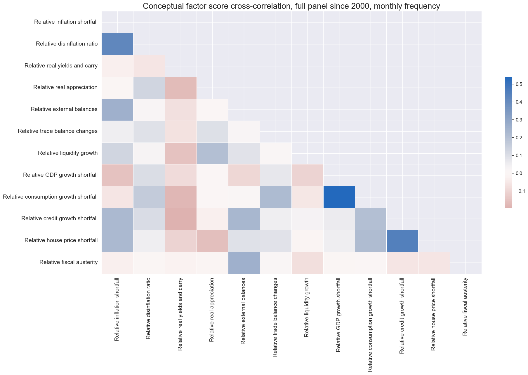
Correlation across the 12 conceptual factors has been quite diverse for the full panel of countries and over the past 25 years. The only pair with an above-50% positive correlation has been relative GDP growth shortfalls and relative consumption growth shortfalls. The two are related and could be combined, but are still conceptually different.

Conceptual parity and machine learning trading signals

A rough analysis of all conceptual factors and 5-year IRS receiver returns reveals positive forward correlation of all of them with subsequent relative vol-targeted returns at a monthly frequency. This is reassuring, considering that they all have theoretical backing and that markets rarely observe relative economic performances in a timely and careful manner. No selection or optimisation was applied in the design process, and no other factors have been tested.

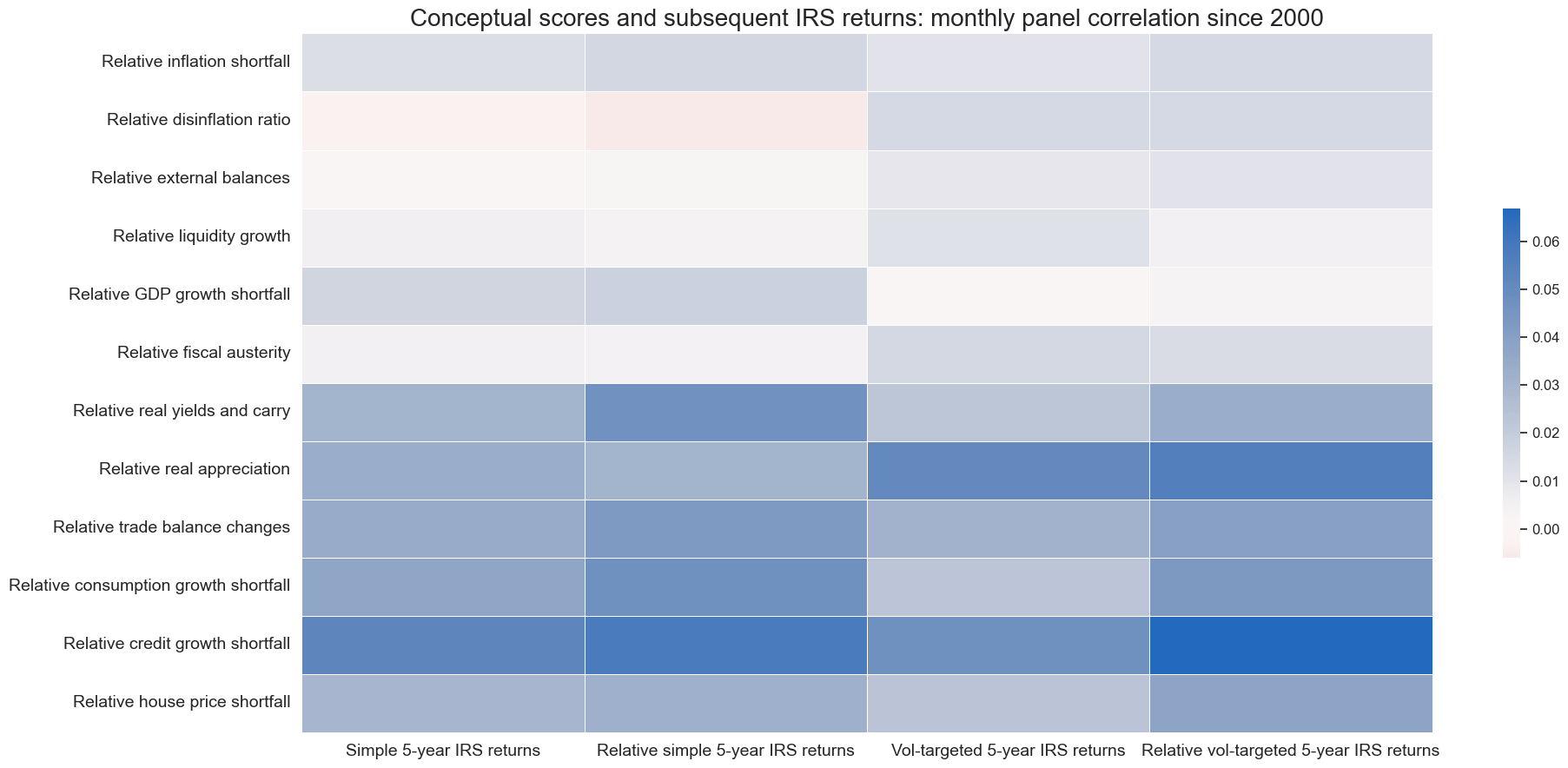
However, the strength of predictive power and cross-correlations has been very different across factors. Hence, a critical step for strategy development is condensing candidate factors into a single positioning signal. Here we consider two valid methods for this step: conceptual parity and sequential machine learning. Valid means that the produced signals are largely free from hindsight and form a sound basis for realistic backtests.

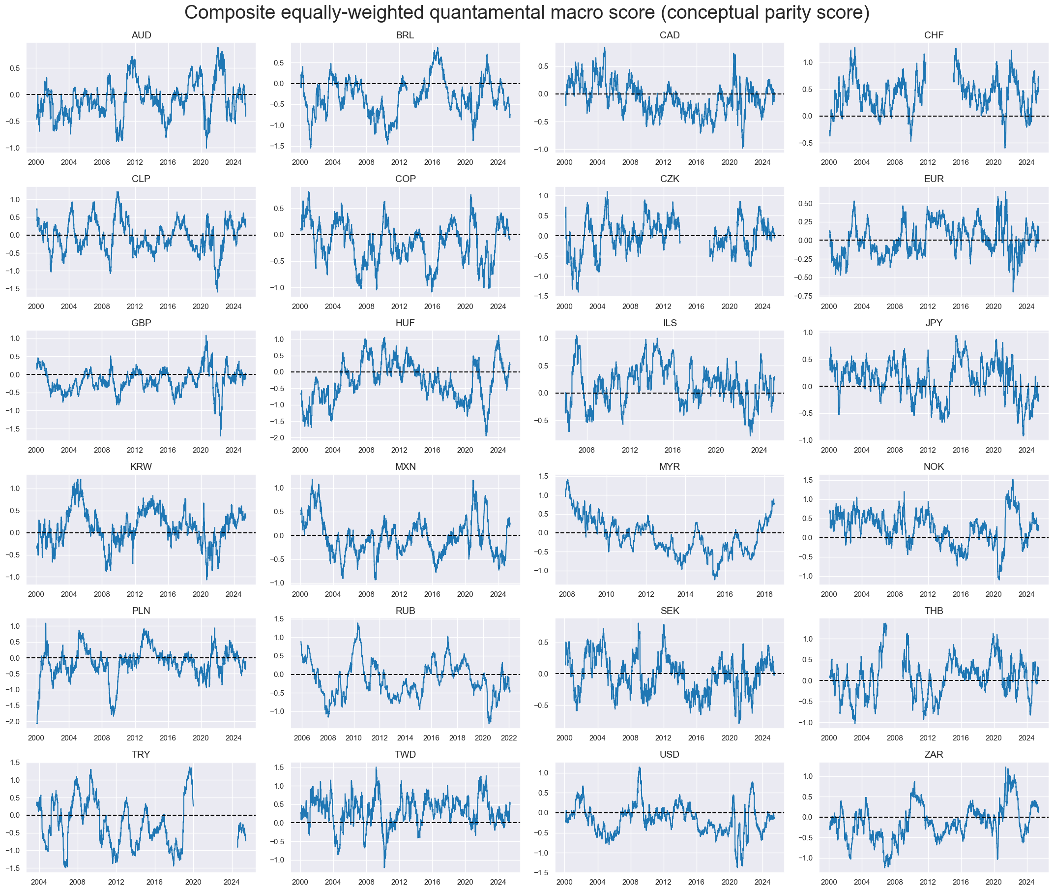
Conceptual parity aggregates groups of factors by first normalising them—typically by expressing values as standard deviations from a neutral baseline—and then averaging the results without consideration of empirical predictive power. This process ensures that each conceptual factor carries equal weight. While brutally simple, this approach is notably robust to shifts in economic regimes and helps mitigate both implicit and explicit hindsight bias. Its effectiveness depends largely on maintaining clear distinctions between different types of economic influences.

The below timeline fact displays conceptual parity scores based on the 12 conceptual macro scores introduced above. Gaps or late starts in the series reflect blacklisted periods. The signals display both pronounced cyclical dynamics and limited short-term volatility. Sign changes for relative cross-country positions are infrequent, with the direction of positions flipping only about once per year and country.

The other valid approach is sequential machine learning, which may uncover insights that go beyond human cognitive limitations. This method is especially useful when there are weak theoretical priors regarding macro-quantamental factors. Unlike arbitrary or hindsight-driven selection of factors and models, sequential machine learning enables more realistic backtesting by simulating a rational, systematic decision-making process—using only the data available at each point in time.

Here we focus on regression-based learning with two types of models: regularised linear regression and random forest regression. The learning processes optimise model parameters and hyperparameters sequentially and produce signals at each point in time based on the regression model that performed best up to that date. The processes thus learn from growing datasets. Here, machine learning-based signal generation is executed in scikit-learn using some bespoke Python classes for macro-quantamental indicators of the Macrosynergy package (see also Macro trading signal optimisation: basic statistical learning methods). The workflow requires four essential steps:

1. We define model and hyperparameter grids in accordance with scikit-learn conventions. These pre-select the eligible set of model classes and other hyperparameters over which the statistical learning process optimises. Optimisation means periodic model selection based on inner cross-validation and expanding samples.
2. We choose an optimisation criterion for sequential model cross-validation based on point-in-time panel data. Here, our criterion is a naïve Sharpe ratio (documentation) based on a simplistic PnL where the trader goes long by a single unit when the signals are positive and short by a single unit when the predictions are negative.
3. We specify time series panel splits for cross-validation within the sequentially growing development data sets, using one of the specialised functions of the Macrosynergy package. Here we use the ExpandingKFoldPanelSplit. Thereby, dates in the development panel data set are divided into n+1 sequential and non-overlapping intervals, resulting in n pairs of training and test sets.
4. We run the actual sequential optimisation with the Macrosynergy package’s specialised class (SignalOptimizer). It applies scikit-learn cross-validation to the specific format of macro-quantamental panel data. Optimisation means to compare and choose models (“inner evaluation”). The sequence of optimal models delivers point-in-time optimised signals.

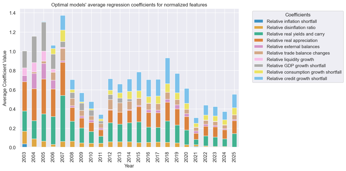
The regularised regression-based learning process uses Ridge regressions with non-negativity constraints on the coefficients of the 12 conceptual factors and various degrees of the regularisation strength (alpha). Over time, the learning processes preferred stricter regularisation and the models converged on five dominant factors: relative credit growth shortfall, relative real appreciation, relative real yields, relative consumption growth shortfall, and relative trade balances changes.

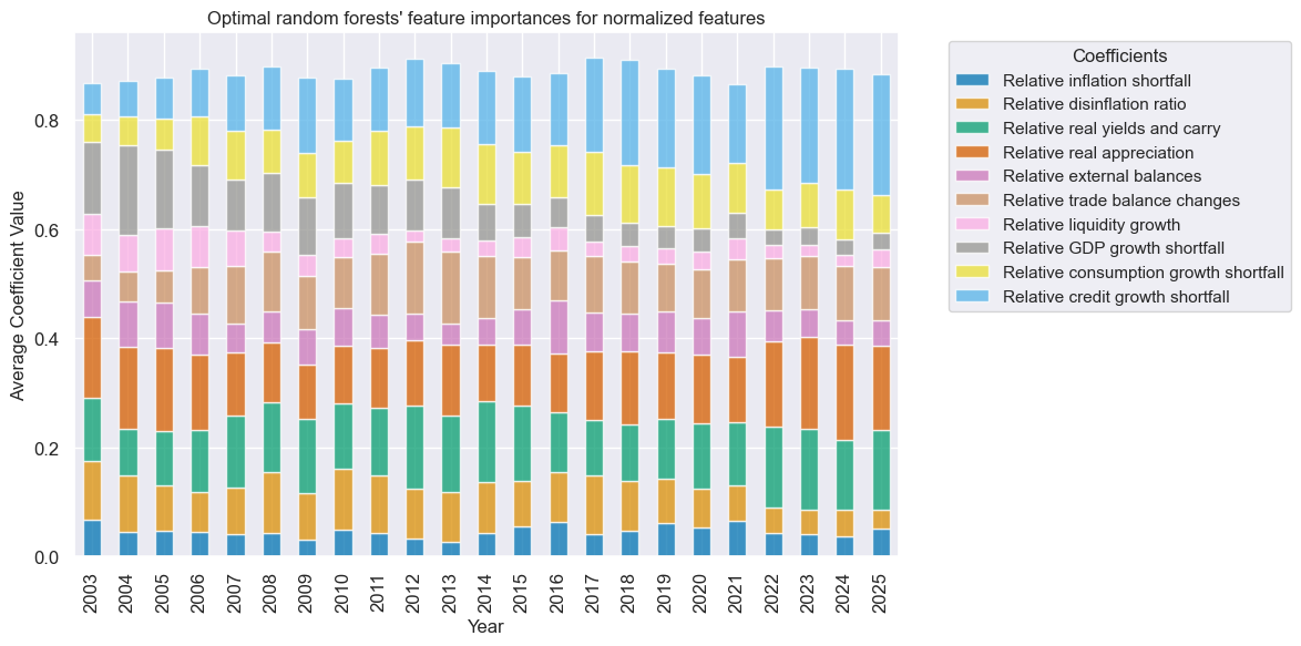
The learning process based on random forest regressions estimates forests with monotonicity constraints that ensure that macro factor scores can only have the theoretically supported direction of impact. Among models the process chooses from [a] “deep” and “shallow” forests, i.e., those that use all or a large share or a small share of the samples for the training of the model, [b] various requirements of the minimum size of a leaf node, and [c] various maxima for the number of features considered when looking for a split. The dominant factors of this learning process are the same as for regularised regression, albeit the weights of the smaller factors are larger.

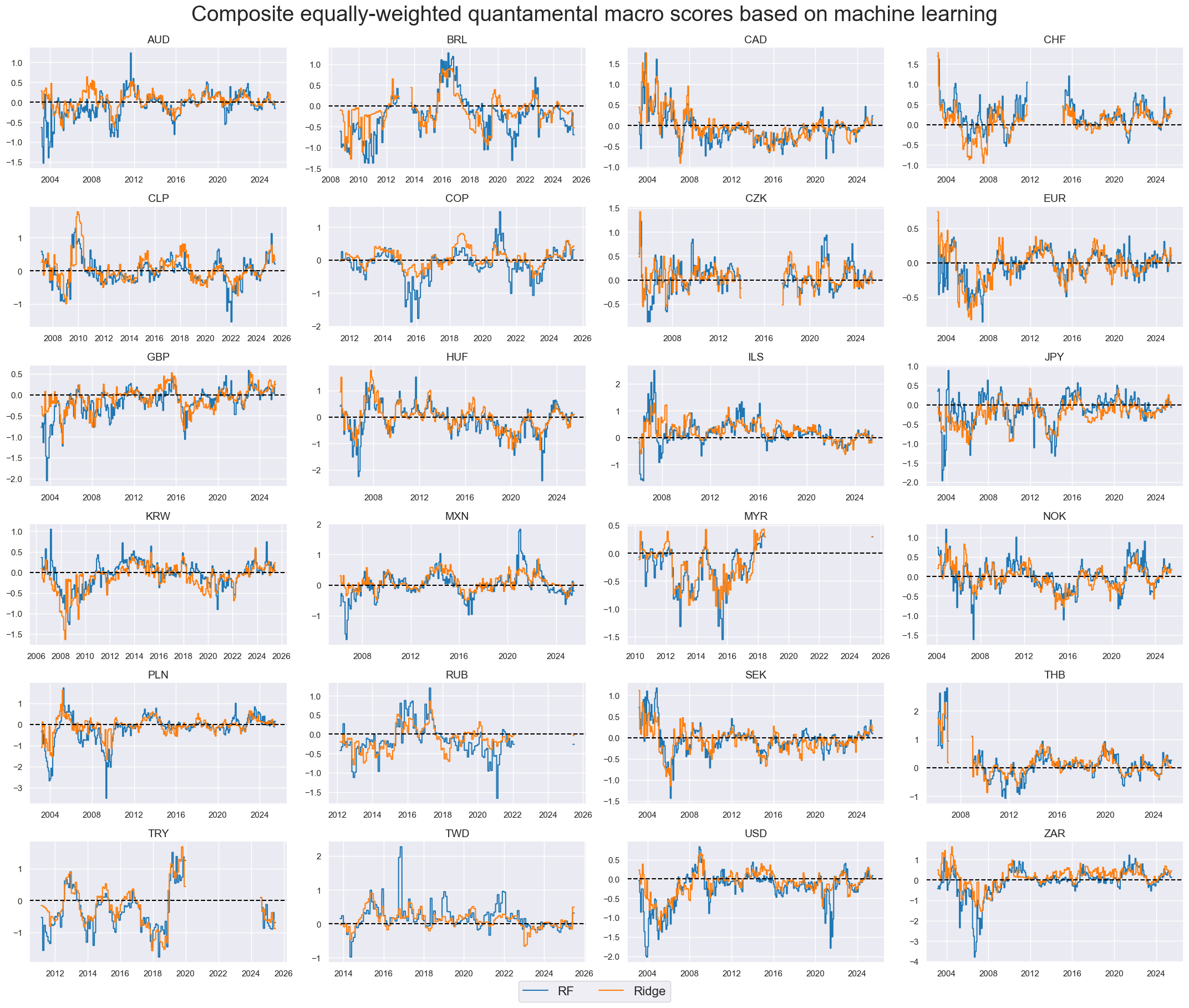
The machine learning-based cross-country IRS trading signals have similar general features to the conceptual parity signal, but values and patterns are at times very different. Generally, machine learning-based signals have a greater proclivity towards surplus volatility than conceptual parity, as variations in signals do not just reflect variations in underlying factors but also changes in deployed models.

The economic value of cross-country RV

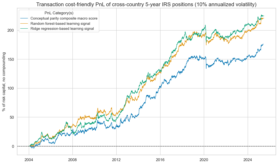
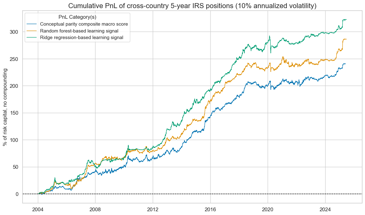
We estimate the economic value of the composite quantamental signals for a cross-country relative value duration strategy by means of a naïve PnL. Positions are taken across all currency areas based on their normalised and winsorised signals with limits of three standard deviations. One unit of signal translates into one unit of volatility-based risk in the reference currency area versus an equally weighted basket of such risk in all concurrently tradable currency areas. Positions are rebalanced monthly at the beginning of the month based on the signal value at the end of the previous month, allowing for one-day slippage for trading. The long-term volatility of the PnL for various signals has been normalised to 10% annualised, for the purpose of graphic displays. Naïve PnL calculation does not consider transaction costs or risk management rules, as those are specific to institutional settings. PnLs could be calculated from 2004, as the first four sample years since 2000 were our minimum data requirement for learning-based signals.

All signal versions produced consistent long-term value since 2004, with less than 5% correlation to U.S. Treasury returns. 21-year Sharpe ratios ranged from 1.1 (conceptual parity) to 1.5 (regularised regressions). Sortino ratios even reached values between 1.7 and 2.3, reflecting the rarity of large drawdowns. PnL generation displayed some seasonality but was not concentrated. The most profitable 5% of months accounted for 35-40% of the overall PnL, which is low for a macro strategy.

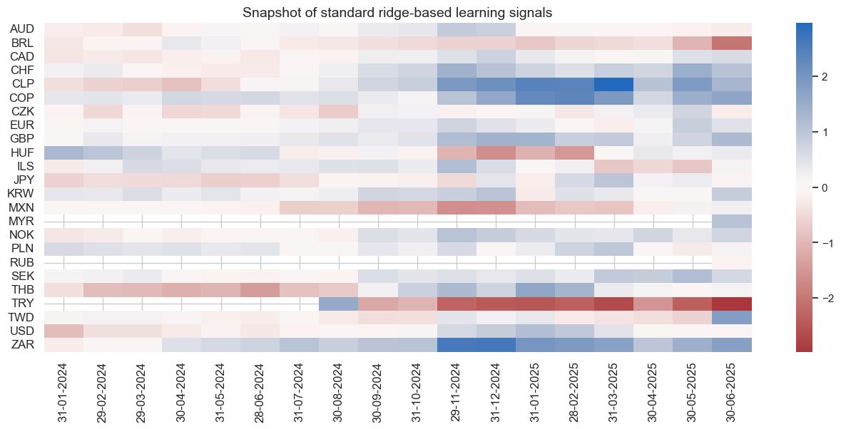
As this strategy relies on leveraged relative positions, transaction costs will reduce performance and limit the scale of risk capital that can be profitably managed with the above simple rules. Fortunately, signals do not normally change aggressively, as illustrated by the snapshot below for the 2024-2025 (June) period.

However, position adjustment is still frequent, and some trading would take place in all places and all months. This can be mitigated by a more transaction cost-friendly version of the strategy that only applies unit long-short signals and imposes thresholds for position taking. As an illustration, we set an entry barrier of a new position at a one standard deviation signal for a country and an exit signal at near zero.

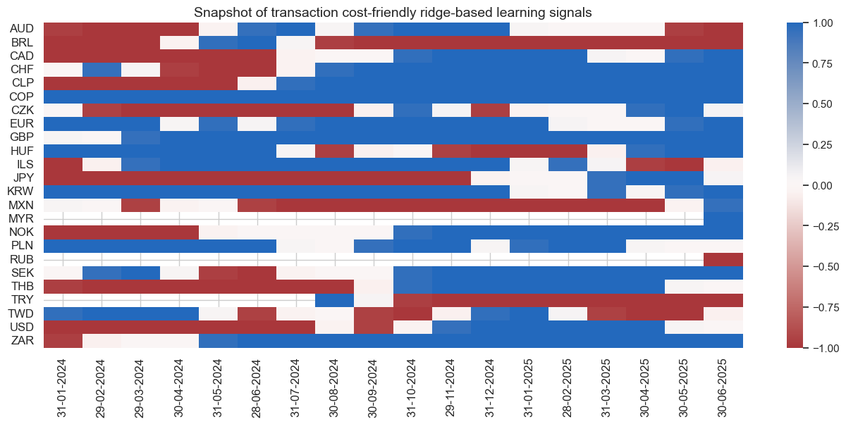
This simplified strategy produces lower risk-adjusted returns but still delivers long-term Sharpe ratios from 0.8 to 1.0 and Sortino ratios from 1.1 to 1.5. None of the naive transaction-cost friendly strategies has any meaningful correlation to the U.S. treasury.