A scorecard for global equity allocation

Jupyter Notebook

Macro-quantamental scorecards are systematic enhancements of discretionary portfolio management. They offer (a) information efficiency by structuring and condensing key macroeconomic data series, and (b) empirical validation of predictive power and trading value using historic point-in-time information. Scorecards can be readily built in Python, with pandas and existing classes and methods.
Macro-quantamental scores support capital allocation across country equity markets, which is critical for long-term wealth generation by professional investment managers and private investors alike. This post demonstrates how to construct a simple tactical scorecard based on real equity carry, real exchange rate valuation, terms-of-trade dynamics, external balance strength, international investment position changes, and economic confidence trends. There is strong evidence that such a systematic approach delivers predictive power and sustained value generation.

The post below is based on Macrosynergy’s proprietary research. Please quote as “Costa, Michele and Sueppel, Ralph, ‘A macro-quantamental scorecard for global equity allocation,’ Macrosynergy research post, September 2025.

A Jupyter notebook for auditing and replicating the research results can be downloaded here. The notebook operation requires access to J.P. Morgan DataQuery to download data from JPMaQS. Everyone with DataQuery access can download data except for the latest months. Moreover, J.P. Morgan offers free trials on the complete dataset for institutional clients. An academic support program sponsors data sets for research projects.

The practical benefits of macro-quantamental scorecards

A macro-quantamental scorecard is a concise, structured presentation of real-time macroeconomic information relevant to a specific financial market segment. Standardised composite “scores” can guide discretionary trading or serve as the foundation for a systematic strategy. The scorecard’s form and structure should be grounded in theory and empirical evidence. Once set up, it allows consistent and systematic use of new economic information. A quick reminder on the meaning of the terms macro-quantamental indicator, category, factor and signal view Annex 1 below.

The defining characteristics of a macro-quantamental scorecard are information efficiency and empirically validated relevance of scores:

• Information efficiency arises from the structuring and condensation of multiple indicators into intuitive scores that are easy to view and interpret. Units are standard deviations from market-neutral levels. Scores are typically produced in comparable forms across countries or currency areas and updated in real time. This enables a continuous and focused review of a wide array of economic indicators at minimal cost in terms of incremental reading time, research, and analysis. Conventional financial research and news media take much longer to ingest and rarely match the scorecards’ broad perspective and systematic rigor.
• Empirical validation means verification of the predictive power and signal value of macro-quantamental scores. The necessary condition for the consideration of certain types of information should always be logic and theory. However, if conviction in theory is weak, it is legitimate to require empirical support as a sufficient condition. Empirical validation increases confidence in the macroeconomic information that we regularly consider for trading. It must be based on point-in-time information on economic indicators, i.e., they are calculated for each day from the time series “vintages” that were available to the market on that day. The primary source for macro-quantamental indicators is the P. Morgan Macrosynergy Quantamental System (JPMaQS), which provides free limited access, trials of full-scale access, and complimentary academic research support. Unlike standard economic point-in-time indicators, quantamental indicators’ predictive power and trading value can be validated quickly and easily (Evaluating macro trading signals in three simple steps).

Thus, the main reasons why macro-quantamental scorecards work are research cost management and scientific rigor. As the volume of quantitative information surges, investor attention becomes scarcer and more valuable. The evaluation and application of information deserve as much care as its production. This is particularly important in the field of macroeconomic information for markets, because macroeconomic effects are pervasive and most traders are not trained economists.

The importance of cross-country equity allocation for wealth generation

In this post, we present a macro-quantamental scorecard designed to guide capital allocation across equity markets in different countries or currency areas. Both professional fund managers and wealth allocators can implement cross-country allocation. Systematically incorporating cross-country economic conditions offers significant long-term benefits.

• Mitigating macro risk concentration: Passive allocation, in the form of global equity indices, is a valid approach as it follows market capitalization and liquidity. However, it also leads to heavy concentration of macro risk in the U.S., which accounts for over 60% of global equity market capitalization (MSCI breakdown). Systematic modification of passive allocation in accordance with actual macroeconomic developments prevents country allocation from becoming fully detached from economic fundamentals.
• Exploiting economic divergences: There is a broad range of economic developments that plausibly affect the relative performance of equity returns in U.S. dollar terms, some of which are captured in the scorecard below. Most of these predict under- and outperformance of countries for a few months or even a year. In a previous post (Systematic equity allocation across countries for dollar-based investors), we applied sequential machine learning to build trading strategies based on such divergences. The purpose was to assess value generation without hindsight and based solely on point-in-time economic information. Empirical evidence based on 19 international markets showed highly significant predictive power and consistent positive PnL generation arising merely from cross-country allocation. Importantly, this type of value generation has been uncorrelated with the overall equity market performance and, hence, principally additive.

Unlike many other macro trading strategies, cross-country equity allocation can be implemented by high-level allocators and private investors. Even investors with modest investable wealth can take country-specific equity exposure through ETFs based on MSCI, FTSE-Russell, and S&P Dow Jones country indices. Given the frequency of directional changes in macroeconomic factors, reallocations can occur at a low frequency, such as quarterly or even annually.

Although the outperformance of global equity portfolios with country allocation rules is subtle in the short run, it can accumulate sizeable added wealth in the long term. For example, one can use the average of the factors used in this post’s scorecard to adjust the weights of countries in a global equity portfolio that consists of 19 developed and emerging markets (see the details of the markets, factors, and equity positions below). The standard approach used in Macrosynergy posts employs a sigmoid function of the average score to derive an adjustment factor that can augment the equal weight by up to two times the original value (for positive score values) or reduce it to zero (for negative score values). A macro-weighted portfolio with quarterly rebalancing has produced an annualized total return of above 12% from 2000 to 2025 (September) compared to 9.6% and 9.9% for an equally-weighted and U.S.-only portfolio. Due to the compounding effects, the outperformance of the macro-weighted fund translated to an additional wealth generation of roughly 700% of the initially invested capital, as illustrated by the chart below.

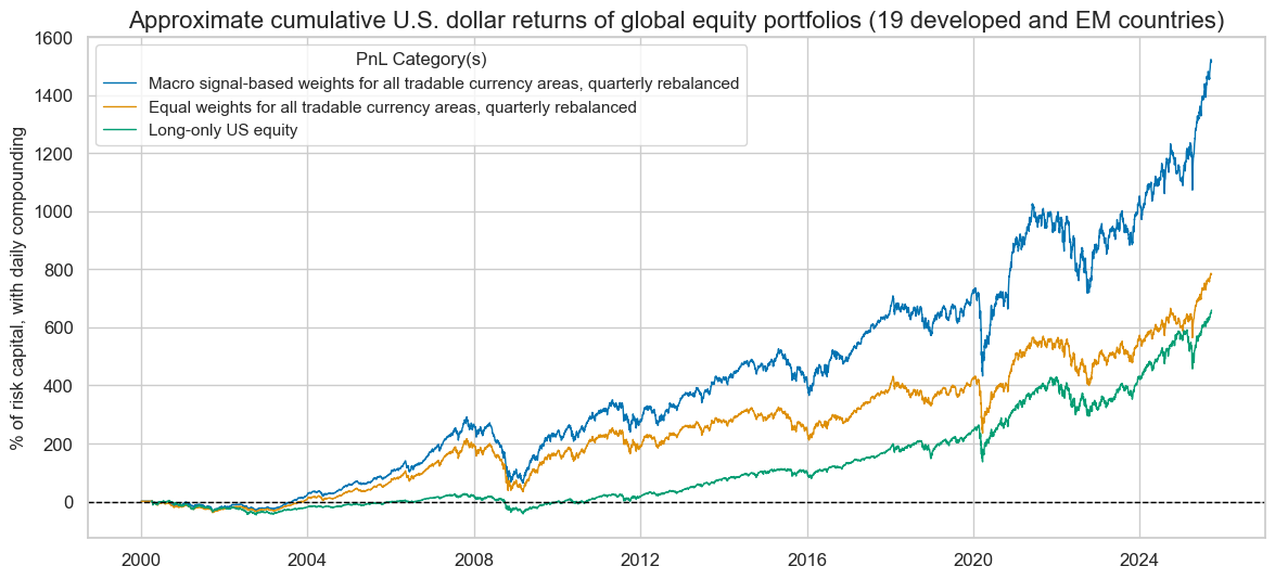
Since factors for the scorecard have been chosen with some empirical hindsight, this value added may be biased to the high side. However, a similar simulation without hindsight, published in the previous machine learning-based post, also produced annual outperformance of total returns of 1-2% per year, which, over a span of 22 years, translated into an additional 500% of the initially invested capital.

A “snapshot scorecard” of macro conditions across countries

“Snapshot scorecards” show the position of various markets according to macro factor scores at any given point in time. If they are based on quantamental indicators, they update daily or even intra-day. The snapshot below compares and ranks USD positions in up to 19 developed and emerging markets:

• The developed market currency areas are (in alphabetical order if the currency symbol): Australia (AUD), Canada (CAD), Switzerland (CHF), the euro area (EUR), the United Kingdom (GBP), Japan (JPY), Sweden (SEK), and the United States (USD).
• The emerging markets are Brazil (BRL), China (CNY), India (INR), South Korea (KRW), Mexico (MXN), Malaysia (MYR), Poland (PLN), Singapore (SGD), Thailand (THB), Taiwan (TWD), and South Africa (ZAR).

The primary targets of allocation and analysis are broad all-cap baskets of stocks across all the above countries, along with their returns in USD terms. They originate from the J.P. Morgan SIFT database (documentation), a dataset comprising pricing and fundamental data for over 20,000 indices, with country indices representing the liquid listed stocks in each of the countries mentioned above. Thus, we simulate the problem of a dollar-based investor that allocates cash across broad equity positions in different currency areas. The factor scores and their composite have been chosen by Macrosynergy for this post and are explained below. However, factor selection and composite calculation should generally reflect the individual portfolio manager’s beliefs, research, and objectives. The post is primarily intended to demonstrate how to construct the scorecard, rather than to assert that the presented form is the best.

The scorecard below ranks and qualifies the tactical position of all tradable markets from a macro-quantamental perspective. Composite scores are simply re-normalized averages of the individual factor scores. On the snapshot date (23 September 2025), two countries displayed positive composite scores above one standard deviation: South Korea and Japan. The macro support for the highest rated Korea was broadly based, and particularly reflected relative improvement in local economic sentiment (compared to the global average), a relatively low real currency value, strong external balance dynamics, and an improving international investment position. Four countries recorded negative composite scores of more than one standard deviation: Malaysia, Mexico, Taiwan, and Brazil. Brazil’s bottom-of-the-league position owed mostly to low real equity carry and relatively poor dynamics of economic sentiment.

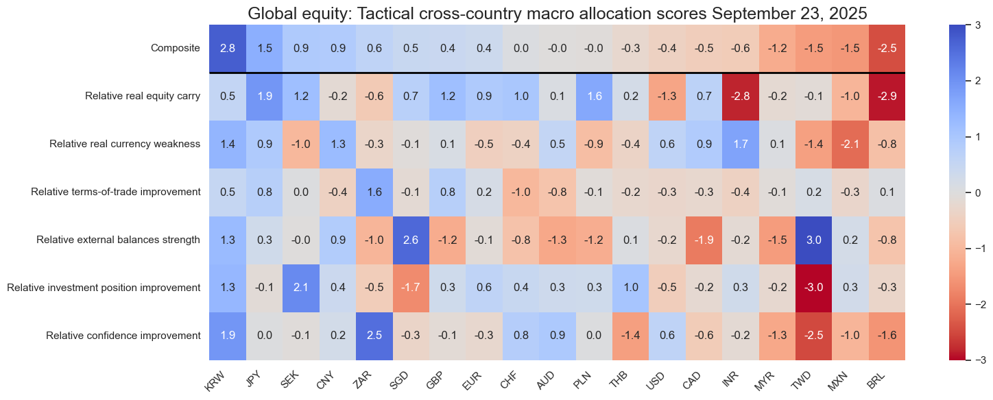
All scorecards in this post can be produced in Python with an appropriate pandas dataframe of quantamental data by using the ScoreVisualisers class of the Macrosynergy package. The snapshot scorecard type can be displayed with the view_snapshot method of the class. The instantiation of the class and the use of the method are shown in the accompanying Jupyter notebook of this post.

The factors of this simple and small scorecard encapsulate a tremendous amount of relevant information in a timely manner. Hence, predictive power plausibly arises from the market’s rational inattention to most encapsulated macro trends. The description and rationale of the individual factor scores are as follows:

• Real equity carry looks at the differential between equity yields, i.e., averages of dividend and equity yields of local indices (documentation), and real interest rates. All other things being equal, relatively high equity yields compared to real funding rates indicate that large premiums are offered for local capital and equity positions. The factor combines nominal equity carry measures with various types of deflators, such as 1-year forward CPI inflation expectations (documentation), annual headline CPI inflation (documentation), core CPI inflation (documentation), and producer price inflation (documentation).
• Real currency weakness measures the negative, inflation-adjusted deviation of a currency’s value from historical or theoretical benchmarks. Real depreciation or undervaluation benefits the competitiveness of local producers and increases the local-currency value of international revenues. This factor combines two types of quantamental categories: shifts relative to purchasing power parity, and openness-adjusted real depreciation.
  • Purchasing power parity-based undervaluation is represented by the percent change of the ratio of the current exchange rate to the PPP(“equilibrium”) over the previous year (documentation).
  • Real openness-adjusted depreciation is measured over multiple horizons: as a percentage of the latest week compared to the previous four weeks, as a percentage of the latest month compared to the same month a year ago, and as a percentage of the latest month compared to the previous 12 months (documentation).
• Terms-of-trade improvements capture short- and medium-term changes in the ratio of exports and import prices. When a country’s output becomes more valuable compared to others, it is more likely to experience stronger growth, better earnings dynamics, and currency appreciation pressure, all of which benefit equity returns in dollar terms. Terms-of-trade dynamics are measured as a percentage of the latest month compared to the same month a year ago, as a percentage of the latest month compared to the previous 1-year average, and as a percentage of the latest week compared to the previous four weeks (documentation).
• External balances strength measures trends of net exports relative to the size of the economy. Rising exports relative to imports often indicate improving competitiveness and reduced exchange rate risks. The constituent categories of the factor are short-term and long-term dynamics of appropriate external balances.
  • As short-term dynamics, we picked changes of seasonally-adjusted merchandise trade balance-to-GDP ratios (6-month moving average over the previous 6 months) and changes in the 12-month merchandise trade balance ratio over the last three reported months (documentation).
  • For long-term trends, we used the latest seasonally adjusted trade and current account balances as a percentage of GDP relative to their 5-year moving averages (documentation here and here).
• Investment position improvements here mean favorable medium-term trends in cross-border investment positions. All other things equal, growing net assets or diminishing international liabilities reduce local financial and currency risk. The conceptual factor is calculated based on two dynamics: the change (over a year ago) of net international investment position as % of GDP (documentation), and the negative change of international liabilities as % of GDP (documentation).
• Confidence improvement captures positive normalized changes in local manufacturing and consumer sentiment survey scores. Brightening sentiment should herald better business conditions and earnings. The underlying macro-quantamental indicators are manufacturing business confidence difference of the last 3 months over the previous 3 months and the difference over a year ago (documentation), as well as consumer confidence differences of the same type (documentation).

All factor scores are based on relative values of quantamental indicators of the local currency areas versus the basket of all 19 countries. Specifically, each relative factor first calculates the relative values of its underlying macro-quantamental categories, then normalizes the relative values sequentially across time and without hindsight around their zero neutral thresholds, then forms an unweighted average of all available relative scores, and finally, re-normalizes that average.

The use of equal weights of the factor scores for the calculation of the composite is motivated solely by the intention to diversify across different macro effects. This mitigates seasonality or value generation, and the risk of relying on a “false positive”, i.e., a factor that looked plausible by theory or empirical analysis, but will fail in the foreseeable future. There has been no optimization of weights.

History scorecard of differences in macro conditions

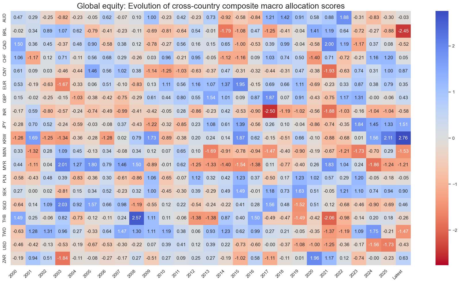
A “history scorecard” characterizes the evolution of macro support for countries over time and puts the current position of countries in perspective. It can be produced with the view_score_evolution method of the ScoreVisualisers Python class.

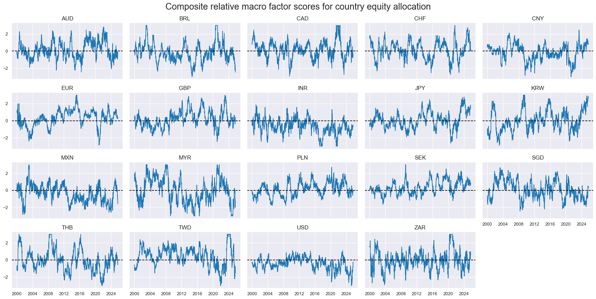
The presentation below displays the annual averages of composite relative macro scores for all 19 equity markets since 2000, as well as for the period from 2025 to date and the latest values. Since the score composites are based on differences between individual currency areas and a global average, there are no predominant positive or negative years. However, the dispersion of scores and the occurrences of large values vary. 2025 appears to be a year with greater-than-normal country differences so far.

The panel of timeline charts below shows the evolution of daily country composite scores since 2000 and highlights their strong autocorrelation. This indicates that relative macroeconomic conditions shift gradually over months or even quarters, rather than from day to day. Changes in the sign of relative conditions for or against specific markets occur infrequently, on average, less than once a year. This testifies to the score’s suitability for low-frequency allocation adjustments.

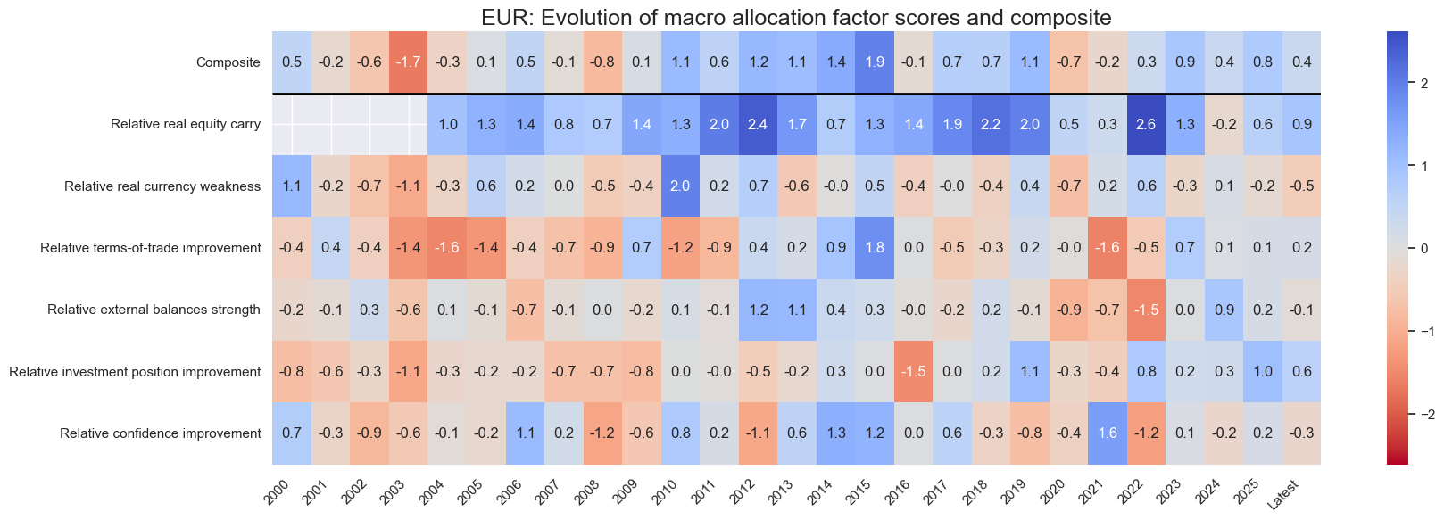
One can display more detailed historical scorecards for individual countries by using the view_cid_evolution of the ScoreVisualisers Python class. For example, macroeconomic conditions for the euro area turned negative during the early 2000s due to a rebounding currency value (as the euro asserted itself), terms-of-trade deterioration (the euro area did not benefit from the rise in commodity prices), and worsening international investment positions. However, conditions turned strongly positive in the wake of the sovereign credit crisis, which led to low real funding costs and elevated equity premia. As the crisis lessened, it ultimately gave way to an improvement in economic confidence.

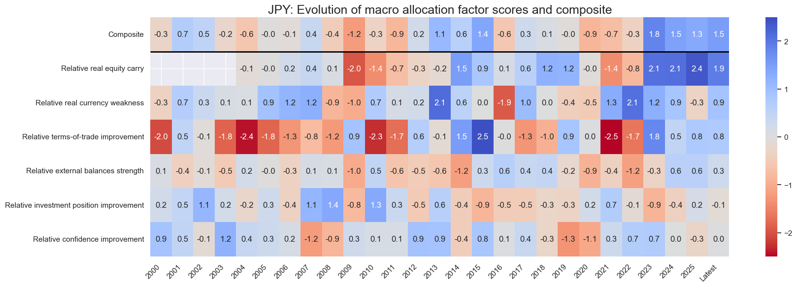
Japan’s macroeconomic scores improved markedly in recent years, reflecting rising real equity yields (as recovering inflation pushed real interest rates down), weakening real currency value, and a relative increase in terms of trade.

Evidence of predictive power and trading value

The purpose of examining the predictive power of factors is to validate their underlying economic rationale and strengthen confidence in the measures. A key advantage of macro-quantamental scores, compared with standard macroeconomic data, is that they are point-in-time and allow to test hypotheses and propositions rigorously. However, empirical validation of selected scores and their composite, on its own, is neither a sufficient nor necessary condition for their consideration in systematic monitoring or trading.

• When we select factors with hindsight, their composite exaggerates predictive power and value generation relative to what we should expect going forward. On its own, such evidence is not a valid ground for adopting the systematic approach. However, evidence that confirms a theoretical proposition is a valid criterion for adopting the proposition. Furthermore, empirical evidence can guide calculations that are not covered by theory, as long as that guidance is not essential for validating the basic approach. Put simply, refinements with hindsight are fine for a scorecard, but valid backtests must be based on unrefined scores or sequential machine learning (view post here).
• Not all macro factor scores need empirical backing. Some highly plausible factors that simply did not show high values and much variation in recent history may be considered going forward due to their potential to shape future market regimes.

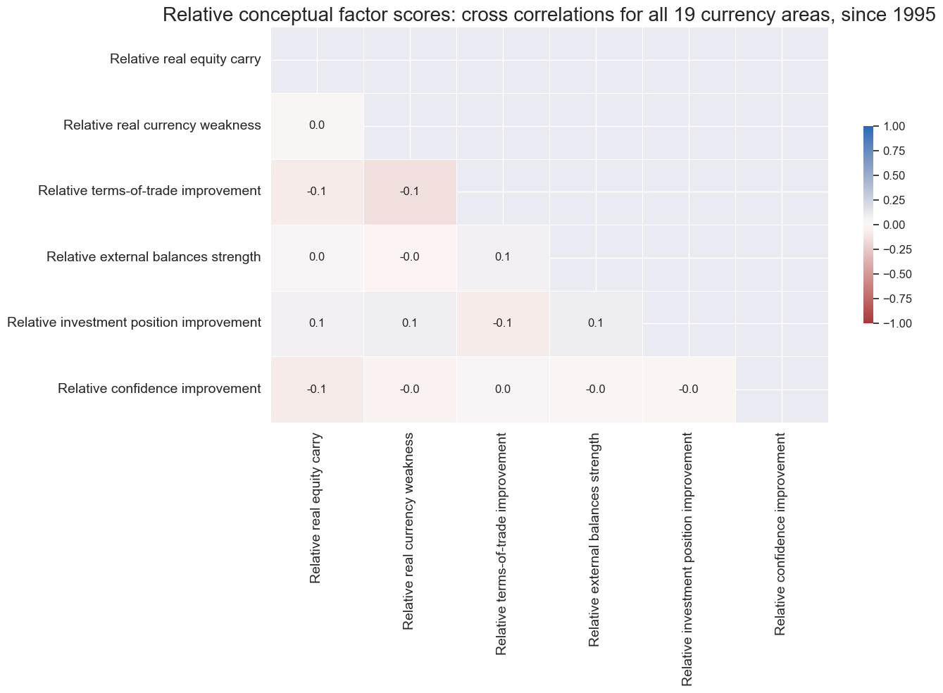
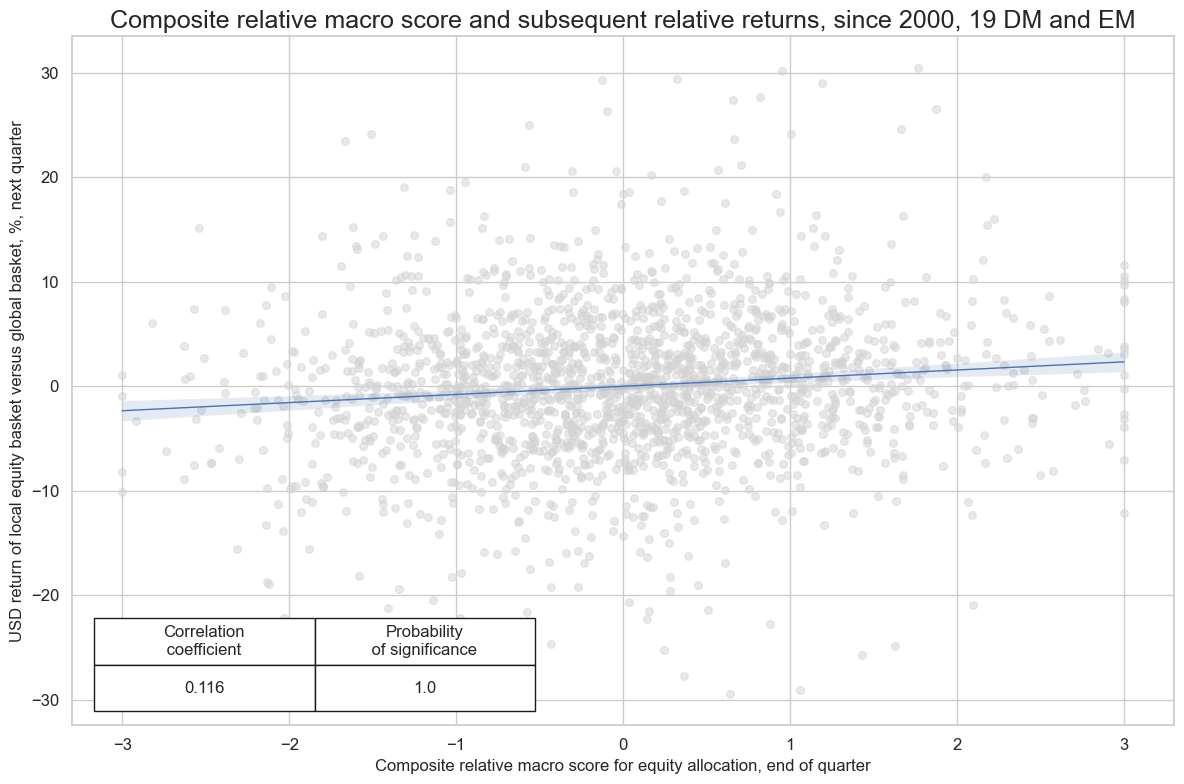
The scatterplot panel below shows quarter-forward correlation coefficients and significance tests of proposed predictive relations using a panel of markets. A relation is significant if end-of-quarter factors across time and country predict the next quarter’s USD equity returns in a way that is unlikely to have happened accidentally. In the case of the relative macro scores for relative cross-country equity returns, the predictive relation has been positive for all six macro factors and highly significant for four of them.

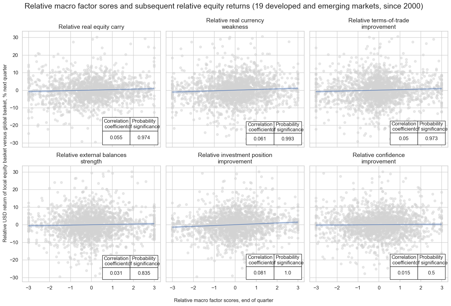
Given the positive predictive relations of all six factors and their low cross-correlation, it is no surprise that the predictive relation of the composite is stronger than that of the best single predictor and is significant with near 100% probability.

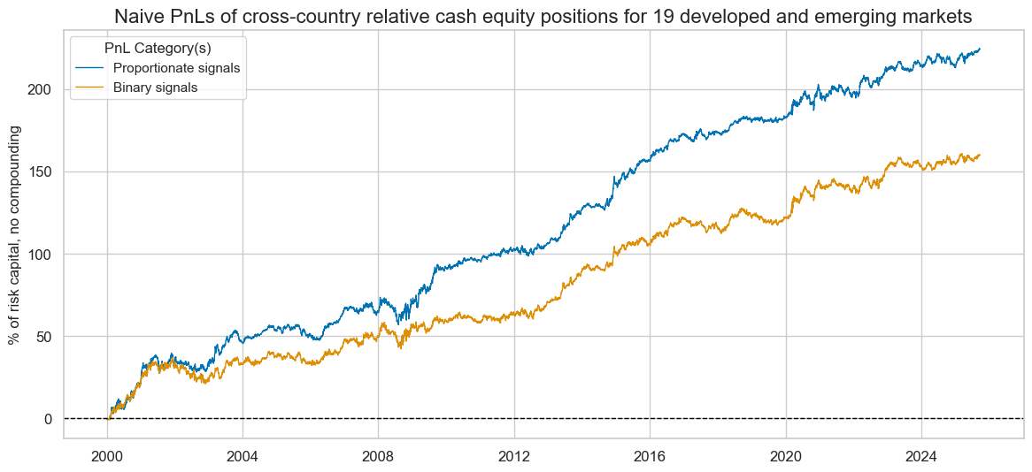
We test the trading value of the composite relative macro factors using a naïve PnL approach of Macrosynergy posts. Month-end signals from the learning process determine relative positions (one country versus an equally weighted equity basket of all) for the start of the next month, with a one-day gap for execution. Signal size is capped at three standard deviations as basic risk control. The PnLs ignore transaction costs and compounding, and are scaled to a 10% annualized volatility for easier return comparison.

The naïve PnL from cross-country positioning without directional exposure has produced a 25-year Sharpe ratio of 0.9 and a Sortino ratio of 1.3. A PnL that uses only binary signals, taking equal positions for each long and short signal, irrespective of the absolute score value, would still have produced a 25-year Sharpe ratio of 0.6 and a Sortino ratio of 0.9.

Annex 1: Terminology

The following terms are used for quantamental data types:

• A macro-quantamental indicator is a metric that combines quantitative and fundamental analysis of the macroeconomy, such as an inflation trend or a government balance-to-GDP ratio. Values must be point-in-time information states, i.e., reflect that state of public knowledge at a timestamp. Here, public knowledge does not mean that everybody actually did know but that everybody could have known what the data said.
• A macro-quantamental category is a time series panel of a macro-quantamental indicator for a set of countries and markets. For example, real-time annual GDP growth estimates across countries constitute a category. Validation of trading strategy principles often relies on categories rather than single indicators to enhance, drawing on the diverse experiences of multiple countries.
• A macro-quantamental factor is a combination of macro-quantamental indicators or categories. The combination is presumed to serve as a predictor of financial contract returns. For example, growth rates of various measures of economic activity may be combined into an “excess activity growth” factor, which is relevant to the performance of fixed-income or equity markets.
• Finally, a macro-quantamental signal is a combination of macro-quantamental factors and possibly other types of factors. The signal is designed to govern risk and positioning in a specific market. For example, an excess activity growth factor and an excess inflation factor in conjunction with real interest rates may be combined into a fixed-income trading signal.

Additional insights into macro-trading strategies can be found here.