Sectoral equity index returns

This category group contains daily local-currency cash equity returns for both country indices and country-specific sector indices. The sectors considered are consumer discretionary goods, consumer staples, communication services, energy, financials, health care, industrials, information technology, materials, real estate, and utilities.

The data is sourced from from the J.P. Morgan SIFT database. JP Morgan Strategic Indices Fundamental Toolkit (SIFT) is a DataQuery dataset consisting of pricing and fundamental data for 20,000+ indices, including JPM North America All-Cap Index, JPM Swedish Small-Cap Real Estate Index, JPM UK Housebuilder Index, and so forth. Based on global stocks since 1986 and North American stocks from the early 1960s, the product is categorized by region/country, market size segment and sector/industry group, as well as different factors including the overall market. The end result is a range of available indices based on a combination of these categorizations, such as Momentum within North American Technology, Value within European Utilities and more. For more information or to request a demo, please contact Data_Analytics_Sales@jpmorgan.com

Equity index total returns in % of notional

Ticker : EQCALLR_NSA / EQCCODR_NSA / EQCCOSR_NSA / EQCCSRR_NSA / EQCENRR_NSA / EQCFINR_NSA / EQCHLCR_NSA / EQCINDR_NSA / EQCITER_NSA / EQCMATR_NSA / EQCRELR_NSA / EQCUTLR_NSA

Label : Equity index return in % of notional: all sectors / consumer discretionary / consumer staples / communication services / energy / financials / healthcare / industrials / information technology / materials / real estate / utilities.

Definition : Return on equity portfolios, value-weighted and rebalanced once a month, % of notional of the contract: all sectors / consumer discretionary / consumer staples / communication services / energy / financials / healthcare / industrials / information technology / materials / real estate / utilities.

Notes :

• The return is simply the % change of the index price.

• See Appendix 1 for the index construction.

Equity index excess returns in % of notional

Ticker : EQCALLXR_NSA / EQCCODXR_NSA / EQCCOSXR_NSA / EQCCSRXR_NSA / EQCENRXR_NSA / EQCFINXR_NSA / EQCHLCXR_NSA / EQCINDXR_NSA / EQCITEXR_NSA / EQCMATXR_NSA / EQCRELXR_NSA / EQCUTLXR_NSA

Label : Equity index excess return in % of notional: all sectors / consumer discretionary / consumer staples / communication services / energy / financials / healthcare / industrials / information technology / materials / real estate / utilities.

Definition : Return in excess of nominal interest rate on equity portfolios, value-weighted and rebalanced once a month, % of notional of the contract: all sectors / consumer discretionary / consumer staples / communication services / energy / financials / healthcare / industrials / information technology / materials / real estate / utilities.

Notes :

• The return is simply the % change of the index price.

• See Appendix 1 for the index construction.

Vol-targeted equity index total returns

Ticker : EQCALLR_VT10 / EQCCODR_VT10 / EQCCOSR_VT10 / EQCCSRR_VT10 / EQCENRR_VT10 / EQCFINR_VT10 / EQCHLCR_VT10 / EQCINDR_VT10 / EQCITER_VT10 / EQCMATR_VT10 / EQCRELR_VT10 / EQCUTLR_VT10

Label : Equity index return for 10% vol target: all sectors / consumer discretionary / consumer staples / communication services / energy / financials / healthcare / industrials / information technology / materials / real estate / utilities.

Definition : Return on equity portfolios, value-weighted and rebalanced once a month, % of risk capital on position scaled to 10% (annualized) volatility target: all sectors / consumer discretionary / consumer staples / communication services / energy / financials / healthcare / industrials / information technology / materials / real estate / utilities.

Notes :

• Positions are scaled to a 10% volatility target based on the historic standard deviation for an exponential moving average with a half-life of 11 days. Positions are rebalanced at the end of each month.

Vol-targeted equity index excess returns

Ticker : EQCALLXR_VT10 / EQCCODXR_VT10 / EQCCOSXR_VT10 / EQCCSRXR_VT10 / EQCENRXR_VT10 / EQCFINXR_VT10 / EQCHLCXR_VT10 / EQCINDXR_VT10 / EQCITEXR_VT10 / EQCMATXR_VT10 / EQCRELXR_VT10 / EQCUTLXR_VT10

Label : Equity index excess return for 10% vol target: all sectors / consumer discretionary / consumer staples / communication services / energy / financials / healthcare / industrials / information technology / materials / real estate / utilities.

Definition : Return in excess of nominal interest rate on equity portfolios, value-weighted and rebalanced once a month, % of risk capital on position scaled to 10% (annualized) volatility target: all sectors / consumer discretionary / consumer staples / communication services / energy / financials / healthcare / industrials / information technology / materials / real estate / utilities.

Notes :

• Positions are scaled to a 10% volatility target based on the historic standard deviation for an exponential moving average with a half-life of 11 days. Positions are rebalanced at the end of each month.

Untradability for equity indices

Ticker : EQCALLUNTRADABLE_NSA / EQCCODUNTRADABLE_NSA / EQCCOSUNTRADABLE_NSA / EQCCSRUNTRADABLE_NSA / EQCENRUNTRADABLE_NSA / EQCFINUNTRADABLE_NSA / EQCHLCUNTRADABLE_NSA / EQCINDUNTRADABLE_NSA / EQCITEUNTRADABLE_NSA / EQCMATUNTRADABLE_NSA / EQCRELUNTRADABLE_NSA / EQCUTLUNTRADABLE_NSA

Label : Equity index untradability and blacklisting: all sectors / consumer discretionary / consumer staples / communication services / energy / financials / healthcare / industrials / information technology / materials / real estate / utilities.

Definition : Untradability binary flag for equity portfolios: all sectors / consumer discretionary / consumer staples / communication services / energy / financials / healthcare / industrials / information technology / materials / real estate / utilities.

Notes :

• Each index has a dynamic set of constituents, that can change over time on the basis of the represenative universe selection criteria. This means that some indices might not have any constituent at a given point in time. This binary indicator allows the user to verify whether the index is dormient (value 1) or active (value 0).

Imports

Only the standard Python data science packages and the specialized macrosynergy package are needed.

import os
import numpy as np
import pandas as pd
import matplotlib.pyplot as plt
import seaborn as sns
import math
import copy
import json

import macrosynergy.management as msm
import macrosynergy.panel as msp
import macrosynergy.signal as mss
import macrosynergy.pnl as msn
import macrosynergy.visuals as msv

from macrosynergy.download import JPMaQSDownload

from timeit import default_timer as timer
from datetime import timedelta, date, datetime

import warnings

warnings.simplefilter("ignore")

The JPMaQS indicators we consider are downloaded using the J.P. Morgan Dataquery API interface within the macrosynergy package. This is done by specifying ticker strings , formed by appending an indicator category code <category> to a currency area code <cross_section> . These constitute the main part of a full quantamental indicator ticker, taking the form DB(JPMAQS,<cross_section>_<category>,<info>) , where <info> denotes the time series of information for the given cross-section and category. The following types of information are available:

• value giving the latest available values for the indicator

• eop_lag referring to days elapsed since the end of the observation period

• mop_lag referring to the number of days elapsed since the mean observation period

• grade denoting a grade of the observation, giving a metric of real time information quality.

After instantiating the JPMaQSDownload class within the macrosynergy.download module, one can use the download(tickers,start_date,metrics) method to easily download the necessary data, where tickers is an array of ticker strings, start_date is the first collection date to be considered and metrics is an array comprising the times series information to be downloaded.

# Cross-sections of interest
cids_dmeq = ['AUD', 'CAD', 'CHF', 'EUR', 'GBP', 'HKD', 'ILS', 'JPY', 'NOK', 'NZD', 'SEK', 'SGD', 'USD']
cids_eueq = ["DEM", "ESP", "FRF", "ITL", "NLG"]
cids_aseq = []
cids_eeeq = []
cids_laeq = []

cids = sorted(cids_dmeq + cids_eueq + cids_aseq + cids_eeeq + cids_laeq)
sector_cids = sorted(cids_dmeq + cids_eueq)

sector_labels = {
    "ALL": "All sectors", 
    "COD": "Cons. discretionary",
    "COS": "Cons. staples",
    "CSR": "Communication services",
    "ENR": "Energy",
    "FIN": "Financials",
    "HLC": "Healthcare",
    "IND": "Industrials",
    "ITE": "Information tech",
    "MAT": "Materials",
    "REL": "Real estate",
    "UTL": "Utilities",
}
sectors = list(sector_labels.keys())
cids_secs = list(sector_labels.keys())[1:]

simple_rets = ["EQC" + sec + "R_NSA" for sec in sectors]
vt_rets = ["EQC" + sec + "R_VT10" for sec in sectors]
simple_xrets = ["EQC" + sec + "XR_NSA" for sec in sectors]
vt_xrets = ["EQC" + sec + "XR_VT10" for sec in sectors] 
untradable = ['EQC' + sec + 'UNTRADABLE_NSA' for sec in sectors]

main = simple_rets + vt_rets + simple_xrets + vt_xrets 
econ = [
    # core consumer inflation: level (YoY) and change (vs last quarter)
    'CPIC_SA_P1M1ML12', 'CPIC_SA_P1M1ML12_D1M1ML3',
    # sentiment surveys: manufacturing, services (level, change over 3 months or 1 quarter)
    "MBCSCORE_SA", "MBCSCORE_SA_D1Q1QL1", "MBCSCORE_SA_D3M3ML3",
    "SBCSCORE_SA", "SBCSCORE_SA_D1Q1QL1", "SBCSCORE_SA_D3M3ML3",
    # FX appreciation
    "REEROADJ_NSA_P1W4WL1", "REEROADJ_NSA_P1M12ML1", "NEEROADJ_NSA_P1W4WL1",
]
mark = untradable  # market links

xcats = main + econ + mark

# Download series from J.P. Morgan DataQuery by tickers

start_date = "1989-12-31"
tickers = [cid + "_" + xcat for cid in cids for xcat in xcats]
print(f"Maximum number of tickers is {len(tickers)}")

# Retrieve credentials

client_id: str = os.getenv("DQ_CLIENT_ID")
client_secret: str = os.getenv("DQ_CLIENT_SECRET")

# Download from DataQuery

with JPMaQSDownload(client_id=client_id, client_secret=client_secret) as downloader:
    start = timer()
    assert downloader.check_connection()
    df = downloader.download(
        tickers=tickers,
        start_date=start_date,
        metrics=["value", "eop_lag", "mop_lag", "grading"],
        suppress_warning=True,
        show_progress=True,
    )
    end = timer()

dfd = df.copy(deep=True)

print("Download time from DQ: " + str(timedelta(seconds=end - start)))

Maximum number of tickers is 1278
Downloading data from JPMaQS.
Timestamp UTC:  2024-03-14 17:00:11
Connection successful!

Requesting data: 100%|██████████| 256/256 [00:59<00:00,  4.29it/s]
Downloading data: 100%|██████████| 256/256 [01:21<00:00,  3.14it/s]  

Some expressions are missing from the downloaded data. Check logger output for complete list.
260 out of 5112 expressions are missing. To download the catalogue of all available expressions and filter the unavailable expressions, set `get_catalogue=True` in the call to `JPMaQSDownload.download()`.
Some dates are missing from the downloaded data. 
10437 out of 19361 dates are missing.
Download time from DQ: 0:02:49.339604

Availability

cids_exp = sector_cids  # cids expected in category panels
msm.missing_in_df(dfd, xcats=main, cids=cids_exp)

Missing xcats across df:  []
Missing cids for EQCALLR_NSA:  []
Missing cids for EQCALLR_VT10:  []
Missing cids for EQCALLXR_NSA:  []
Missing cids for EQCALLXR_VT10:  []
Missing cids for EQCCODR_NSA:  []
Missing cids for EQCCODR_VT10:  []
Missing cids for EQCCODXR_NSA:  []
Missing cids for EQCCODXR_VT10:  []
Missing cids for EQCCOSR_NSA:  []
Missing cids for EQCCOSR_VT10:  []
Missing cids for EQCCOSXR_NSA:  []
Missing cids for EQCCOSXR_VT10:  []
Missing cids for EQCCSRR_NSA:  []
Missing cids for EQCCSRR_VT10:  []
Missing cids for EQCCSRXR_NSA:  []
Missing cids for EQCCSRXR_VT10:  []
Missing cids for EQCENRR_NSA:  ['CHF']
Missing cids for EQCENRR_VT10:  ['CHF']
Missing cids for EQCENRXR_NSA:  ['CHF']
Missing cids for EQCENRXR_VT10:  ['CHF']
Missing cids for EQCFINR_NSA:  []
Missing cids for EQCFINR_VT10:  []
Missing cids for EQCFINXR_NSA:  []
Missing cids for EQCFINXR_VT10:  []
Missing cids for EQCHLCR_NSA:  []
Missing cids for EQCHLCR_VT10:  []
Missing cids for EQCHLCXR_NSA:  []
Missing cids for EQCHLCXR_VT10:  []
Missing cids for EQCINDR_NSA:  []
Missing cids for EQCINDR_VT10:  []
Missing cids for EQCINDXR_NSA:  []
Missing cids for EQCINDXR_VT10:  []
Missing cids for EQCITER_NSA:  []
Missing cids for EQCITER_VT10:  []
Missing cids for EQCITEXR_NSA:  []
Missing cids for EQCITEXR_VT10:  []
Missing cids for EQCMATR_NSA:  []
Missing cids for EQCMATR_VT10:  []
Missing cids for EQCMATXR_NSA:  []
Missing cids for EQCMATXR_VT10:  []
Missing cids for EQCRELR_NSA:  []
Missing cids for EQCRELR_VT10:  []
Missing cids for EQCRELXR_NSA:  []
Missing cids for EQCRELXR_VT10:  []
Missing cids for EQCUTLR_NSA:  []
Missing cids for EQCUTLR_VT10:  []
Missing cids for EQCUTLXR_NSA:  []
Missing cids for EQCUTLXR_VT10:  []

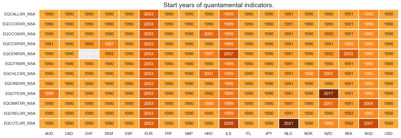
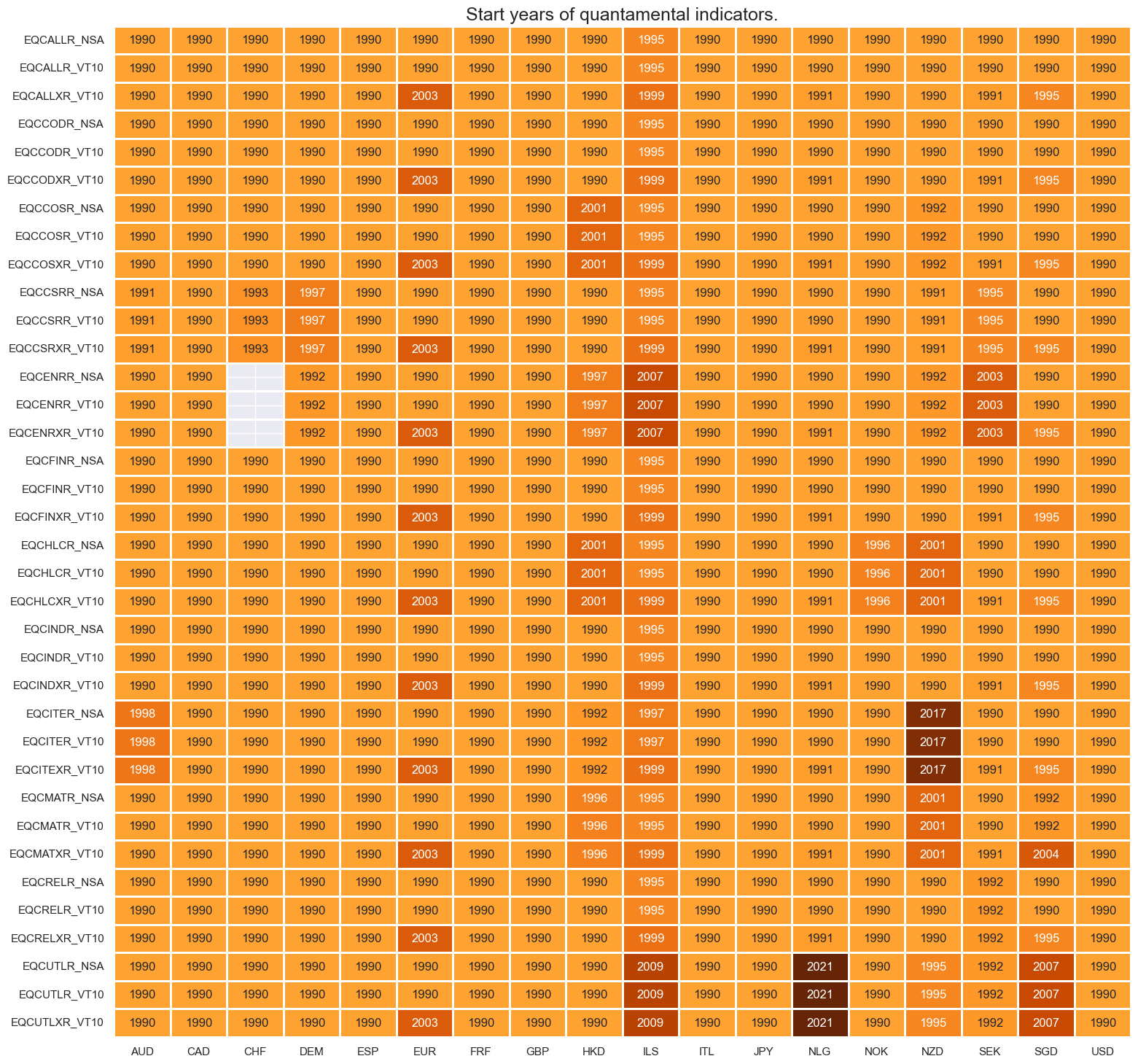
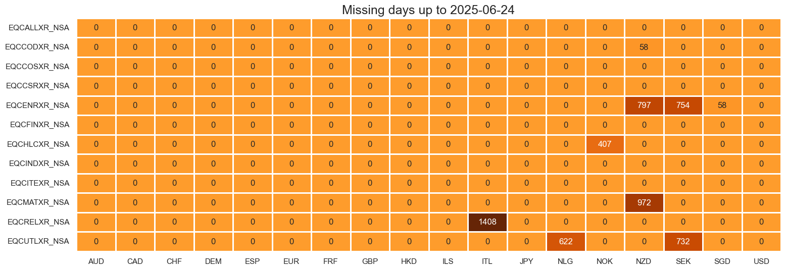
Both general and sectoral equity indices have a deep history as well as an almost complete cross sectional coverage, with most of developed economies recording liquid stock markets since the early 1990s. There are a few exceptions: Switzerland does not have any listed company in the energy GICS sector. In early periods, some industries in Hong Kong, Israel, New Zealand, and Singapore have zero or not enough constituents, so the series start later on. For the explanation of index construction and universe selection, please view Appendix 1 . For the explanation of geographical and sectoral composition, please refer to Appendix 2 and Appendix 3 .

xcatx = [xc for xc in main if xc.endswith("XR_NSA")]
cidx = cids_exp

dfx = msm.reduce_df(dfd, xcats=xcatx, cids=cidx)
dfs = msm.check_startyears(
    dfx,
)
msm.visual_paneldates(dfs)

print("Last updated:", date.today())

Last updated: 2024-03-14

The availability of excess returns is sometimes constrained by nominal interest rates, even though the simple return indicators have longer history as in the case for European economies.

xcatx = [xc for xc in main if not xc.endswith("XR_NSA")]
cidx = cids_exp

dfx = msm.reduce_df(dfd, xcats=xcatx, cids=cidx)
dfs = msm.check_startyears(
    dfx,
)
msm.visual_paneldates(dfs)

print("Last updated:", date.today())

Last updated: 2024-03-14

xcatx = [xc for xc in main if xc.endswith("XR_NSA")]
cidx = cids_exp

plot = msm.check_availability(
    dfd, xcats=xcatx, cids=cidx, start_size=(18, 1), start_years=False
)

xcatx = [xc for xc in main if xc.endswith("XR_NSA")]
cidx = cids_exp

plot = msp.heatmap_grades(
    dfd,
    xcats=xcatx,
    cids=cidx,
    size=(18, 6),
    title=f"Average vintage grades from {start_date} onwards",
)

xcatx = ["EQCALLR_NSA"]
cidx = cids_exp

msp.view_ranges(
    dfd,
    xcats=xcatx,
    cids=cidx,
    val="eop_lag",
    title="End of observation period lags (ranges of time elapsed since end of observation period in days)",
    start=start_date,
    kind="box",
    size=(16, 4),
)

History

Sectoral equity index returns in % of notional

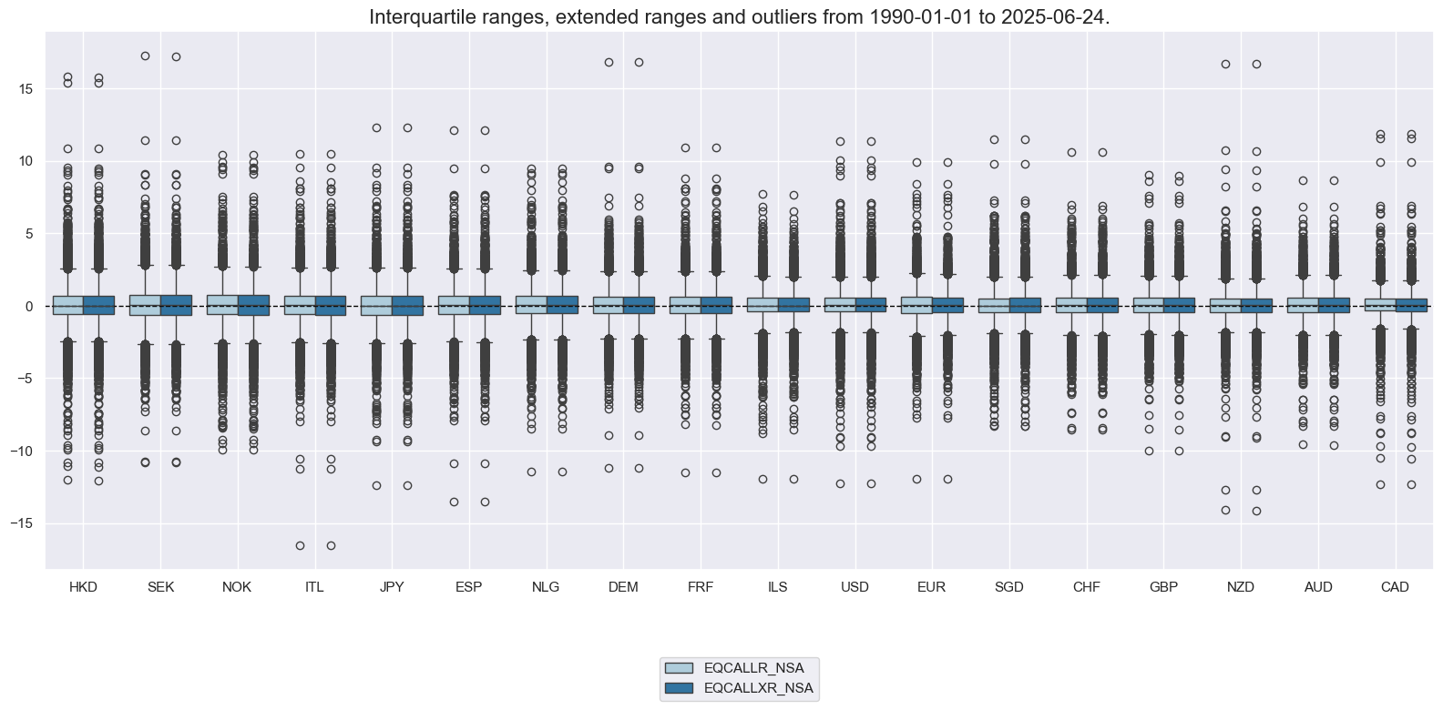
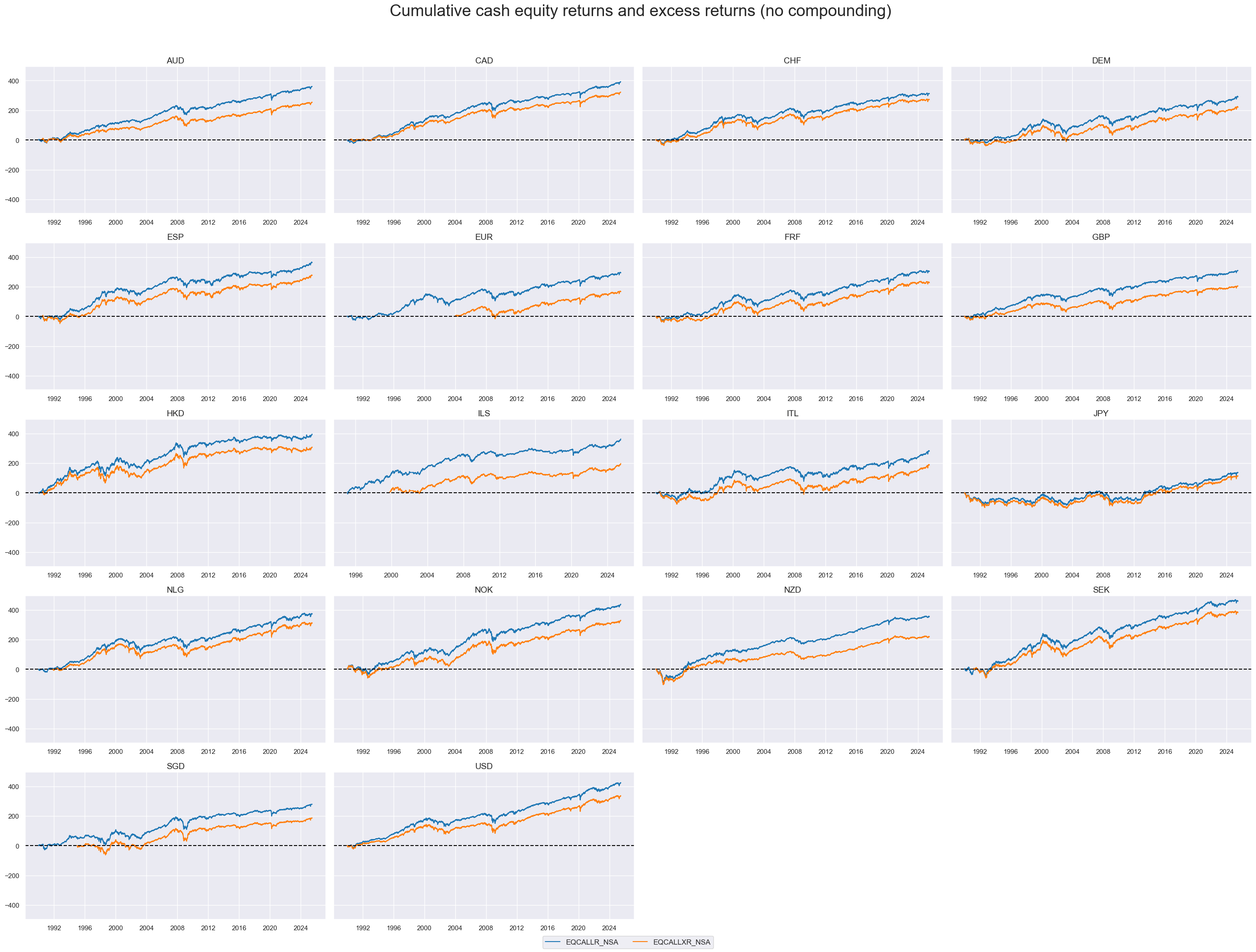
Equity index returns and excess returns have displayed standard deviations and proclicity to outliers of similar orders of magnitude across countries. All countries recorded substantially positive returns and excess returns throughout the period, with the exception of Japan until early 2010s.

xcatx = ["EQCALLR_NSA", "EQCALLXR_NSA"]
cidx = cids_exp

msp.view_ranges(
    dfd,
    xcats=xcatx,
    cids=cidx,
    sort_cids_by="std",
    start=start_date,
    kind="box",
    title=None,
    xcat_labels=None,
    size=(16, 8),
)

xcatx = ["EQCALLR_NSA", "EQCALLXR_NSA"]
cidx = cids_exp
start_date = "1990-01-01"

msp.view_timelines(
    dfd,
    xcats=xcatx,
    cids=cidx,
    start=start_date,
    title="Cumulative cash equity returns and excess returns (no compounding)",
    title_fontsize=27,
    title_adj=1.02,
    title_xadj=0.51,
    cumsum=True,
    ncol=4,
    same_y=True,
    size=(12, 7),
    aspect=1.7,
    all_xticks=True,
)

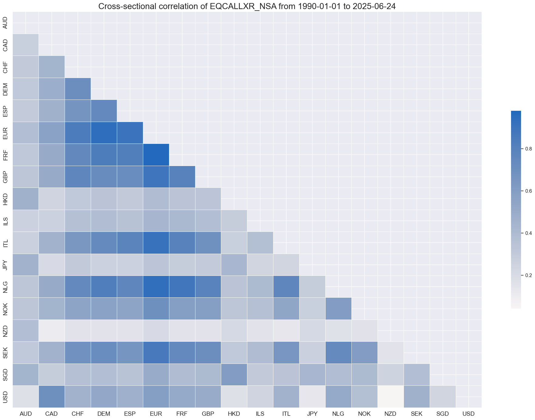
Equity indices returns tend to co-move substantially, reflecting the interconnectedness of global equity markets. Some regions like Israel, Japan, and New Zealand have a slightly lower correlation.

xcatx = "EQCALLXR_NSA"
cidx = cids_exp

msp.correl_matrix(
    dfd,
    xcats=xcatx,
    cids=cidx,
    title=None,
    size=(20, 14),
)

Vol-targeted equity index future returns

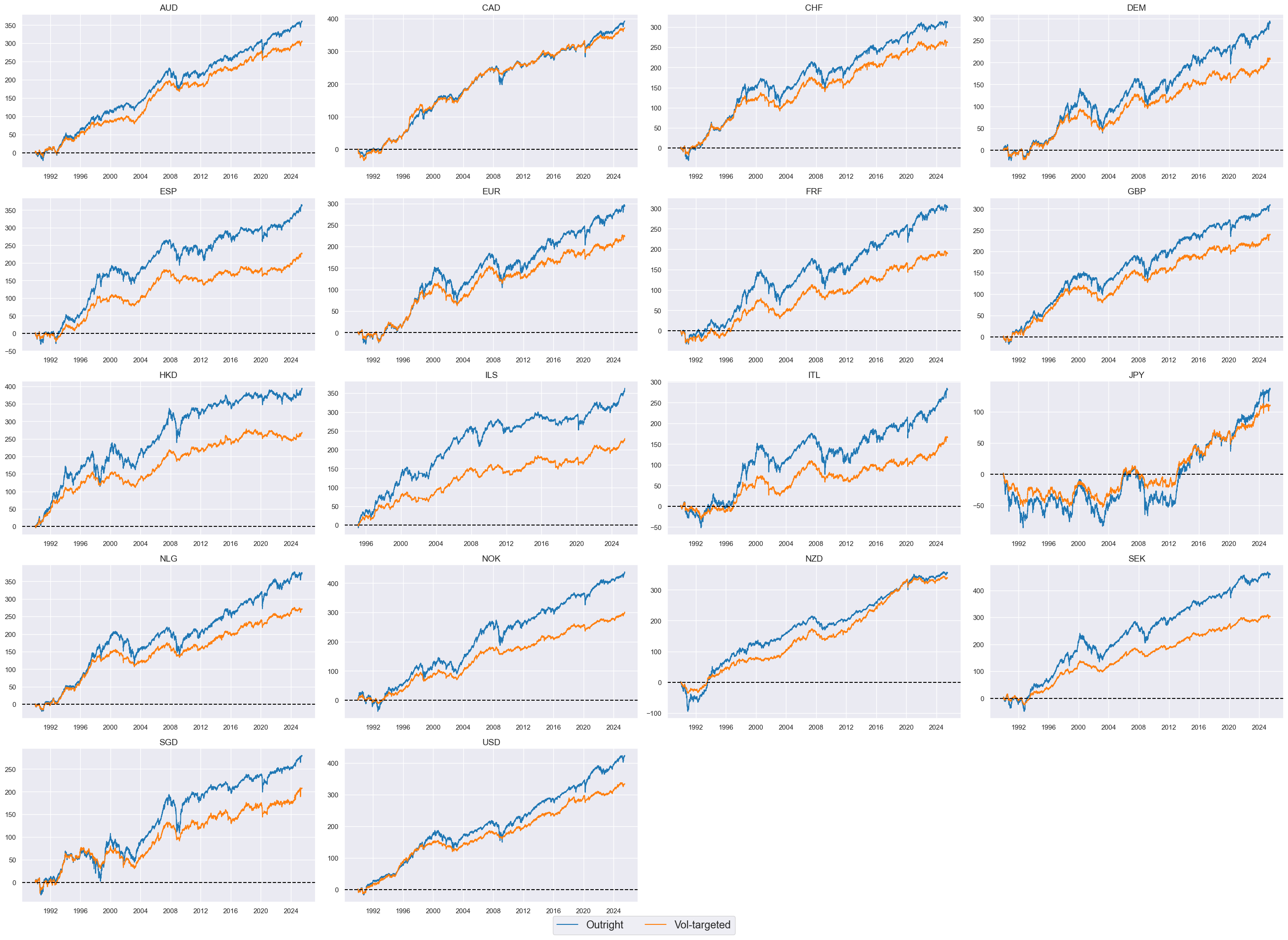
Vol-targeted returns allow comparisons of vol-adjusted returns and are basis for many relative cross-country or cross-sector strategies. In most markets a 10% volatility target with monthly rebalancing would have noticeably reduced long-term returns. The exception is New Zealand, where targeted and non-targeted returns were similar.

xcatx = ["EQCALLR_NSA", "EQCALLR_VT10"]
cidx = cids_exp

msp.view_timelines(
    dfd,
    xcats=xcatx,
    cids=cidx,
    start=start_date,
    title=None,
    xcat_labels=["Outright", "Vol-targeted"],
    title_adj=1.02,
    title_xadj=0.45,
    legend_fontsize=17,
    label_adj=0.075,
    title_fontsize=27,
    cumsum=True,
    ncol=4,
    same_y=False,
    size=(12, 7),
    aspect=1.7,
    all_xticks=True,
)

Importance

Research Links

“Our empirical analysis shows that strategies based on intermediate past returns yield higher mean returns. Moreover, strategies involving both return specifications exhibit time-varying factor exposures, especially when applying the Fama and French (2015) five-factor model. After risk-adjusting for these dynamic exposures, the profitability of industry momentum strategies diminishes and becomes insignificant for strategies based on recent past returns. However, most strategies built on intermediate past returns remain profitable and highly significant. … We find profits of industry momentum strategies to be related to market states and to the business cycle.” Huhn

“Recent empirical evidence has demonstrated that both global industry factors and country factors are important determinants of equity prices.” Cavaglia Moroz

“Cross-region and cross-sector asset allocation decisions are one of the most fundamental issues in international equity portfolio management.” Dou et al.

Transformations

# replacing the category code with equivalent ones to allow cross-country comparisons below
dict_repl = {
    "MBCSCORE_SA_D1Q1QL1": "MBCSCORE_SA_D3M3ML3",
    "SBCSCORE_SA_D1Q1QL1": "SBCSCORE_SA_D3M3ML3",
}
for key, value in dict_repl.items():
    dfd["xcat"] = dfd["xcat"].str.replace(key, value)
    
# dropping the categories replaced from the indicators' set
econ = list(set(econ) - set(dict_repl.keys()))

# not using the European single countries to avoid double counting when averaging
cids_exp = cids_dmeq

# starting in 2000
start_date = "1999-12-31"

# Adjusting by untradability flag: where flag=1 values are set to NaNs

# support column for the category match
dfd['sector'] = dfd['xcat'].str[0:6]

# finding untradable category
untradable_df = dfd.loc[dfd['xcat'].str.endswith('UNTRADABLE_NSA'), :]
# finding return categories
ret_df = dfd.loc[dfd['xcat'].isin(main), :]

# excluding it from the target dataset
dfd = dfd.loc[
    (~dfd['xcat'].str.endswith('UNTRADABLE_NSA')) & (~dfd['xcat'].isin(main))
]
# merging the two
ret_df = ret_df.merge(
    untradable_df.loc[:, ['real_date', 'cid', 'sector', 'value']].rename(columns={'value': 'untrad'}), 
    on=['real_date', 'cid', 'sector'], 
    how='left'
)

# finding where indices have no constituents
mask = (ret_df['untrad'] == 1)
ret_df.loc[mask, 'value'] = np.NaN

# cleaning
ret_df = ret_df.drop(columns=['untrad', 'sector'])

# re-adding the returns back into dfd
dfd = msm.update_df(dfd, ret_df)
xcats = list(set(xcats) - set(untradable))

Economic indicators relative to global averages

xcatx = econ
cidx = cids_exp

dfa = msp.make_relative_value(
    dfd,
    xcats=xcatx,
    cids=cidx,
    blacklist=None,
    rel_meth="subtract",
    rel_xcats=None,
    postfix="vGLB",
)

dfd = msm.update_df(dfd, dfa)

The category, CPIC_SA_P1M1ML12, is missing ['HKD'] from the requested basket. The new basket will be ['AUD', 'CAD', 'CHF', 'EUR', 'GBP', 'ILS', 'JPY', 'NOK', 'NZD', 'SEK', 'SGD', 'USD'].
The category, SBCSCORE_SA, is missing ['NOK'] from the requested basket. The new basket will be ['AUD', 'CAD', 'CHF', 'EUR', 'GBP', 'ILS', 'JPY', 'NZD', 'SEK', 'SGD', 'USD'].

Sectoral index returns relative to global averages

xcatx = simple_rets + vt_rets + simple_xrets + vt_xrets
cidx = list(set(cids_exp))

dfa = msp.make_relative_value(
    dfd,
    xcats=xcatx,
    cids=cidx,
    blacklist=None,
    rel_meth="subtract",
    rel_xcats=None,
    postfix="vGLB",
)

dfd = msm.update_df(dfd, dfa)

The category, EQCENRR_NSA, is missing ['CHF'] from the requested basket. The new basket will be ['AUD', 'CAD', 'EUR', 'GBP', 'HKD', 'ILS', 'JPY', 'NOK', 'NZD', 'SEK', 'SGD', 'USD'].

xcatx = ['EQCALLXR_NSAvGLB', 'EQCALLXR_VT10vGLB']
cidx = cids_exp

msp.view_timelines(
    dfd,
    xcats=xcatx,
    cids=cidx,
    start=start_date,
    title=None,
    title_fontsize=27,
    title_adj=1.02,
    title_xadj=0.5,
    cumsum=True,
    ncol=4,
    same_y=True,
    size=(12, 7),
    aspect=1.7,
    all_xticks=True,
)

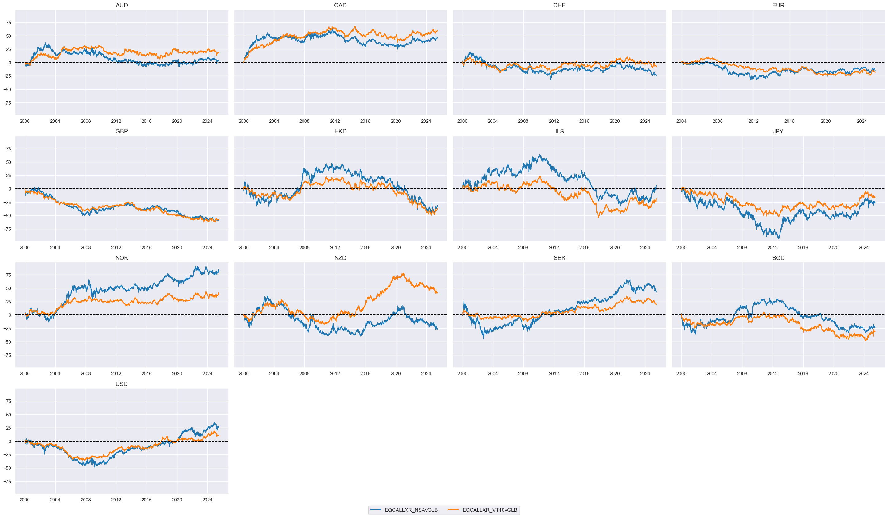
Relative sectoral index returns

rets = ['R_VT10', 'XR_VT10']

calcs = []

for ret in rets:
    calcs_new = [f"EQC{sec}{ret}vALL = EQC{sec}{ret} - EQCALL{ret}" for sec in cids_secs]
    calcs.extend(calcs_new)

dfa = msp.panel_calculator(dfd, calcs, cids=cids_exp)
dfd = msm.update_df(dfd, dfa)

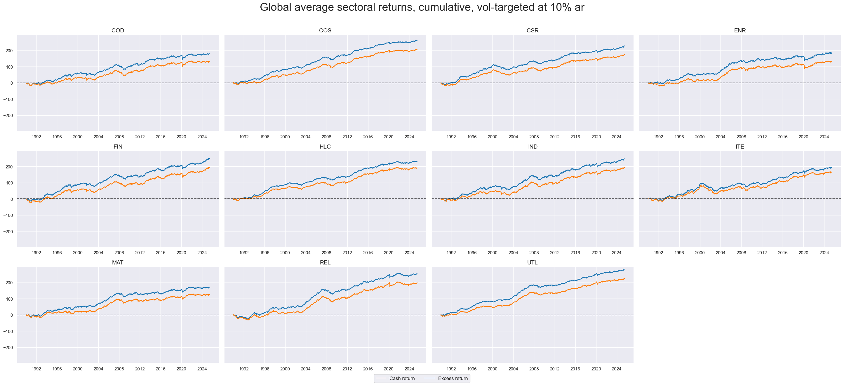
Sectoral indices have shown a relatively different path even if upward-trending. This could reflect the different nature of the businesses, both in terms of cyclical and long-term trajectories.

# Creating a global aggregate return indicator for each sector

xcatx = simple_rets + vt_rets + simple_xrets + vt_xrets
target_cids = cids_exp

global_returns = []
dfa = pd.DataFrame(columns=list(dfd.columns))
for xc in xcatx:
    cidx = copy.deepcopy(
        list(
            set(dfd.loc[dfd['xcat'] == xc, 'cid'].unique()).intersection(target_cids)
        )
    )
    sector_cid = xc[3:6]
    global_sector_cat = xc.replace(sector_cid, "GLB")
    
    # equal weighting the volatility of sector X across all countries in the set
    dfaa = msp.linear_composite(
        df=dfd,
        xcats=xc,
        cids=cidx,
        weights=None,
        new_cid=sector_cid,
        complete_cids=False,
        complete_xcats=False,
    )
    dfaa['xcat'] = global_sector_cat
    
    dfa = msm.update_df(dfa, dfaa)
    global_returns.extend([global_sector_cat])

global_returns = list(set(global_returns))
dfd = msm.update_df(dfd, dfa)

xcatx = ['EQCGLBR_VT10', 'EQCGLBXR_VT10']
cidx = cids_secs
start_date="1990-01-01"


msp.view_timelines(
    dfd,
    xcats=xcatx,
    cids=cidx,
    start=start_date,
    title="Global average sectoral returns, cumulative, vol-targeted at 10% ar",
    title_fontsize=27,
    title_adj=1.02,
    title_xadj=0.5,
    cumsum=True,
    ncol=4,
    same_y=True,
    size=(12, 7),
    aspect=1.7,
    all_xticks=True,
    xcat_grid=False,
    xcat_labels=["Cash return", "Excess return"],
)

Empirical Clues

Effects of openness-adjusted real appreciation

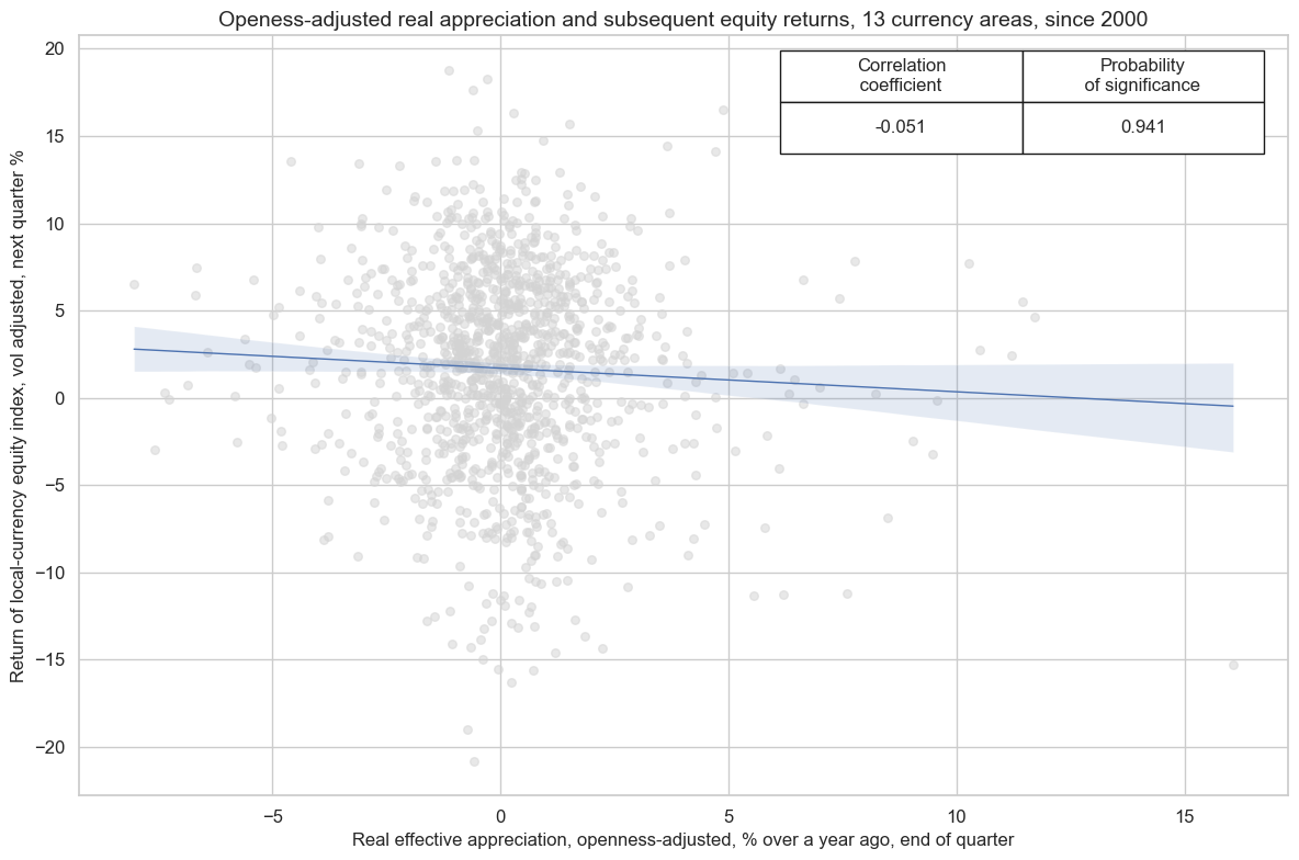
Real effective appreciation plausibly affects corporate earnings negatively, since at least part of revenues of locally listed companies come from exports or foreign subsidiaries. In conjunction with some rational inattention to the continuous changes of real currency values real appreciation should also predict equity returns negatively. For a panel analysis of this relation we use openness-adjusted real appreciation, which modifies appreciation rates by the share of foreign trade to GDP ( view documentation here ). Small open economies and their corporate revenues should be more affected by the same rate of real exchange rate change.

Indeed, a panel regression test shows a signficant negative relation between annual openness-adjusted real appreciation and subsequent quarterly equity returns of aggregate local equity indices.

cidx = cids_dmeq
xcatx = ['REEROADJ_NSA_P1M12ML1', "EQCALLR_VT10"]
start_date = "2000-01-01"

aggregate_eq_cr = msp.CategoryRelations(
    dfd,
    xcats=xcatx,
    cids=cidx,
    freq="Q",
    lag=1,
    xcat_aggs=["last", "sum"],
    start=start_date,
)

aggregate_eq_cr.reg_scatter(
    title="Openess-adjusted real appreciation and subsequent equity returns, 13 currency areas, since 2000",
    labels=False,
    xlab="Real effective appreciation, openness-adjusted, % over a year ago, end of quarter",
    ylab="Return of local-currency equity index, vol adjusted, next quarter %",
    coef_box="upper right",
    prob_est="map",
    fit_reg=True,
    reg_robust=False,
    single_chart=True,
)

REEROADJ_NSA_P1M12ML1 misses: ['HKD'].

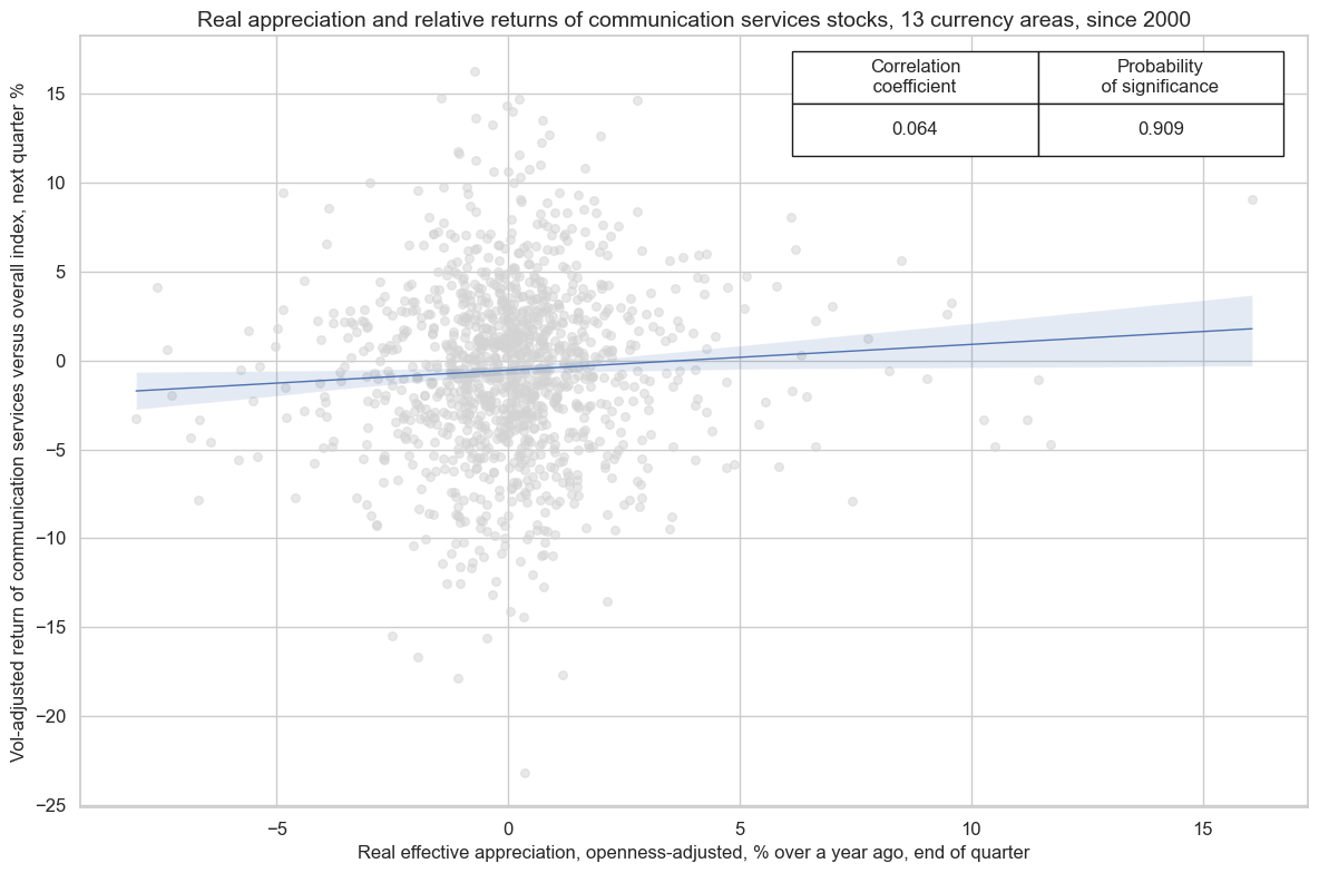
The predictive relationship between openness-adjusted appreciation and equity returns has been negative across most sectos but particularly strong for consumer staples, information technology, and materials. It has been weakest or even positive for sectors that focus on domestic markets, such as communication services, real estate and utilities. These sectors often receiver smaller shares of their revenues in foreign currency and are less subject to foreign competition.

cidx = list(set(cids_dmeq) - set(["HKD"]))
start_date = "2000-01-01"

reer_sector_dict = {}
for sector in sectors:
    xcatx = ["REEROADJ_NSA_P1M12ML1", f"EQC{sector}R_VT10"]
    reer_sector_cr = msp.CategoryRelations(
        dfd,
        xcats=xcatx,
        cids=cidx,
        freq="Q",
        lag=1,
        xcat_aggs=["last", "sum"],
        start=start_date,
    )
    reer_sector_dict[sector] = reer_sector_cr

msv.multiple_reg_scatter(
    cat_rels=list(reer_sector_dict.values()),
    ncol=4,
    nrow=3,
    figsize=(20, 15),
    title="Openness-adjusted real appreciation and subsequent sectoral equity returns, 12 currency areas, since 2000",
    title_xadj=0.5,
    title_yadj=0.99,
    title_fontsize=20,
    xlab="Real effective appreciation, openness-adjusted, % over a year ago, end of quarter",
    ylab="Return of local-currency equity index, vol adjusted, next quarter, %",
    coef_box="upper right",
    prob_est="map",
    single_chart=True,
    subplot_titles=[sector_labels[sector] for sector in sectors]
)

EQCENRR_VT10 misses: ['CHF'].

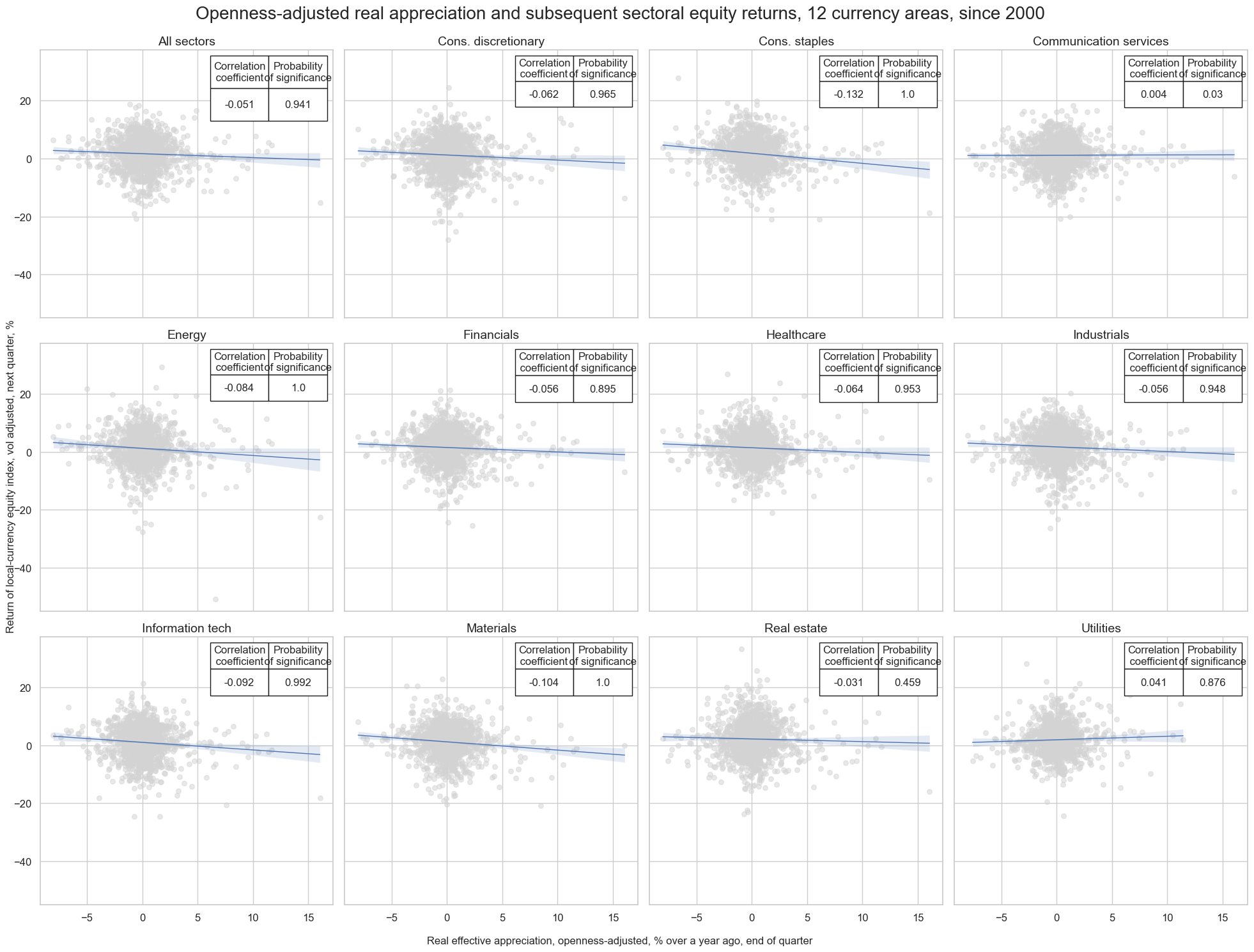
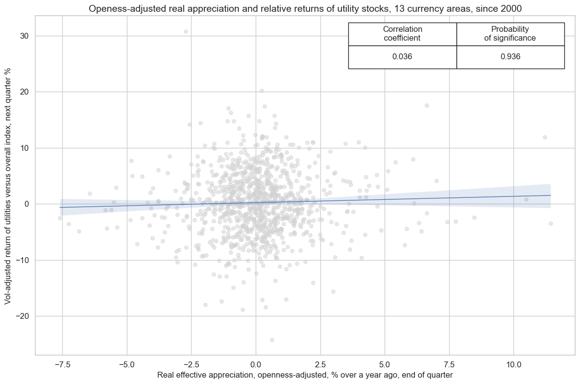
The consequence of the theoretical and empirical divergence of real appreciation effects of different sectors is that openness-adjusted real appreciation serves as a valid signal for the outperformance of domestically-oriented sectors, such as utilities. Real appreciation has been a significant positive predictor of relative returns of utility companies versus the overall local equity index.

cidx = cids_dmeq
xcatx = ['REEROADJ_NSA_P1M12ML1', "EQCUTLR_VT10vALL"]
start_date = "2000-01-01"

aggregate_eq_cr = msp.CategoryRelations(
    dfd,
    xcats=xcatx,
    cids=cidx,
    freq="Q",
    lag=1,
    xcat_aggs=["last", "sum"],
    start=start_date,
)

aggregate_eq_cr.reg_scatter(
    title="Openess-adjusted real appreciation and relative returns of utility stocks, 13 currency areas, since 2000",
    labels=False,
    xlab="Real effective appreciation, openness-adjusted, % over a year ago, end of quarter",
    ylab="Vol-adjusted return of utilities versus overall index, next quarter %",
    coef_box="upper right",
    prob_est="map",
    fit_reg=True,
    reg_robust=False,
    single_chart=True,
)

REEROADJ_NSA_P1M12ML1 misses: ['HKD'].

cidx = cids_dmeq
xcatx = ['REEROADJ_NSA_P1M12ML1', "EQCCSRR_VT10vALL"]
start_date = "2000-01-01"

aggregate_eq_cr = msp.CategoryRelations(
    dfd,
    xcats=xcatx,
    cids=cidx,
    freq="Q",
    lag=1,
    xcat_aggs=["last", "sum"],
    start=start_date,
)

aggregate_eq_cr.reg_scatter(
    title="Real appreciation and relative returns of communication services stocks, 13 currency areas, since 2000",
    labels=False,
    xlab="Real effective appreciation, openness-adjusted, % over a year ago, end of quarter",
    ylab="Vol-adjusted return of communication services versus overall index, next quarter %",
    coef_box="upper right",
    prob_est="map",
    fit_reg=True,
    reg_robust=False,
    single_chart=True,
)

REEROADJ_NSA_P1M12ML1 misses: ['HKD'].

Effects of services business sentiment scores

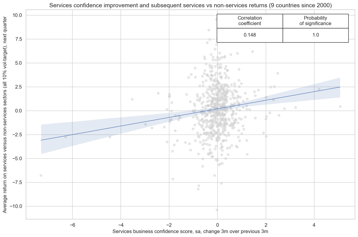
JPMaQS contains services business confidence scores based on various national surveys. Improvements in services business sentiment, measured for example as the change of the last 3 months over the previous three months, have been highly significant predictors of average returns on stocks in services sectors (communication, financials, healthcare, and real estate) relative to average returns in all other sectors, both at a monthly or quarterly frequency.

service_gics = ["CSR", "FIN", "HLC", "REL"]
nonservice_gics = list(set(sectors) - {"CSR", "FIN", "HLC", "REL", "ALL"})

service_rets = [f"EQC{sect}R_VT10" for sect in service_gics]
nonservice_rets = [f"EQC{sect}R_VT10" for sect in nonservice_gics]
calcs = [
    f"EQCSERvNSVR_VT10 = (( {' + '.join(service_rets)} ) / {str(len(service_rets))}) - (( {' + '.join(nonservice_rets)} ) / {str(len(nonservice_rets))})",
]

dfa = msp.panel_calculator(dfd, calcs=calcs, cids=cids_exp)
dfd = msm.update_df(dfd, dfa)

cidx = cids_exp
xcatx = ['SBCSCORE_SA_D3M3ML3', "EQCSERvNSVR_VT10"]
start_date = "2000-01-01"

services_cr = msp.CategoryRelations(
    dfd,
    xcats=xcatx,
    cids=cidx,
    freq="Q",
    lag=1,
    xcat_aggs=["last", "sum"],
    start=start_date,
)

services_cr.reg_scatter(
    title="Services confidence improvement and subsequent services vs non-services returns (9 countries since 2000)",
    labels=False,
    xlab="Services business confidence score, sa, change 3m over previous 3m",
    ylab="Average return on services versus non-services sectors (all 10% vol-target), next quarter",
    coef_box="upper right",
    prob_est="pool",
    fit_reg=True,
    reg_robust=False,
    single_chart=True,
)

SBCSCORE_SA_D3M3ML3 misses: ['HKD', 'NOK'].
EQCSERvNSVR_VT10 misses: ['CHF', 'SEK'].

Effects of manufacturing sentiment scores

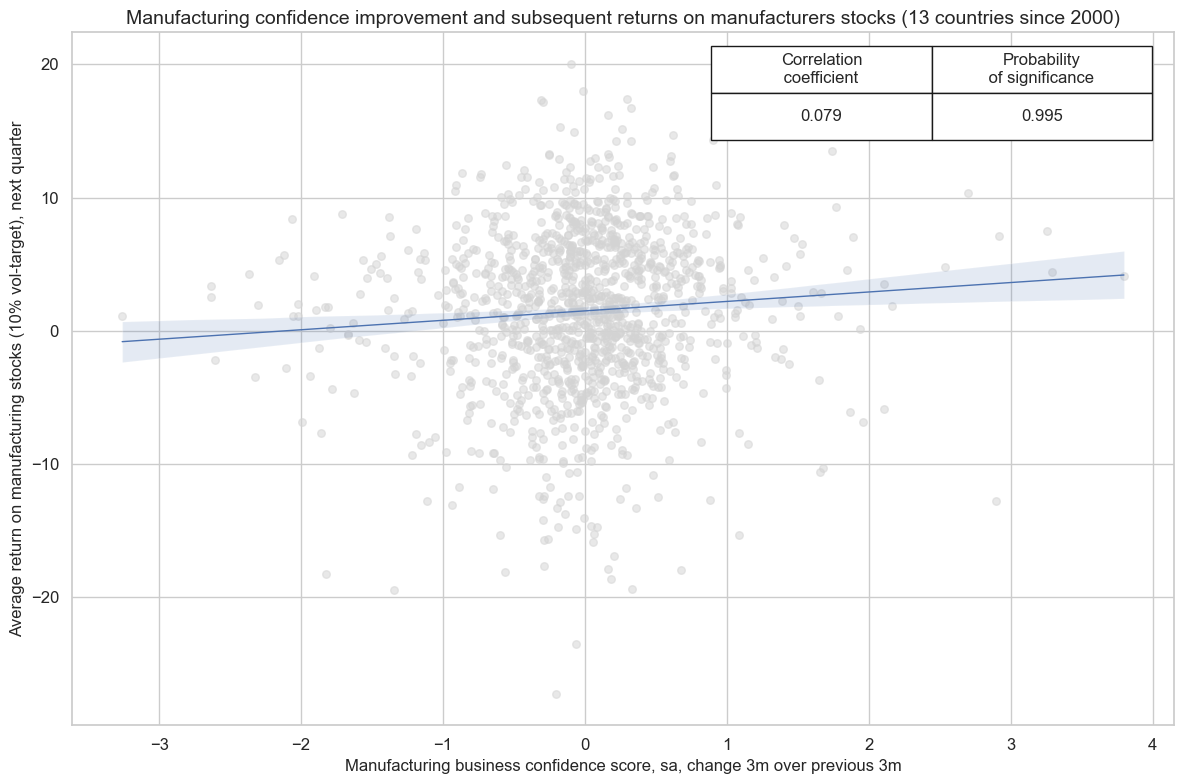
JPMaQS also calculates point-in-time manufactoring business confidence scores based on one or more surveys per country. Increases in manufacturing confidence, measured for example as the change of the last 3 months over the previous three months, have been highly significant predictors of returns in manufacturing stocks. Statistical significance has been high at both monthly and quarterly frequencies.

cids = cids_exp
xcatx = ['MBCSCORE_SA_D3M3ML3', "EQCINDXR_VT10"]
start_date = "2000-01-01"

industrial_cr = msp.CategoryRelations(
    dfd,
    xcats=xcatx,
    cids=cidx,
    freq="Q",
    lag=1,
    xcat_aggs=["last", "sum"],
    start=start_date,
)

industrial_cr.reg_scatter(
    title="Manufacturing confidence improvement and subsequent returns on manufacturers stocks (13 countries since 2000)",
    labels=False,
    xlab="Manufacturing business confidence score, sa, change 3m over previous 3m",
    ylab="Average return on manufacturing stocks (10% vol-target), next quarter",
    coef_box="upper right",
    prob_est="pool",
    fit_reg=True,
    reg_robust=False,
    single_chart=True,
)

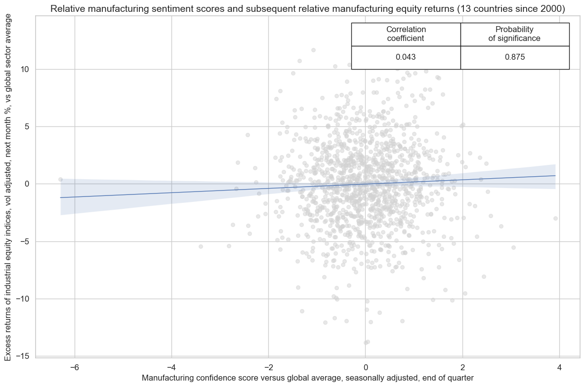
Also, manufacturing sentiment positively predicts relative returns on manufacturing stocks in one country versus others. For relative cross-country positions relative levels have been better predictors than relative changes, which is intuitive because levels of scores are more comparable across surveys.

cids = cids_exp
xcatx = ['MBCSCORE_SAvGLB', "EQCINDXR_VT10vGLB"]
start_date = "2000-01-01"

relative_industrial_cr = msp.CategoryRelations(
    dfd,
    xcats=xcatx,
    cids=cidx,
    freq="Q",
    lag=1,
    xcat_aggs=["last", "sum"],
    start=start_date,
)

relative_industrial_cr.reg_scatter(
    title="Relative manufacturing sentiment scores and subsequent relative manufacturing equity returns (13 countries since 2000)",
    labels=False,
    xlab="Manufacturing confidence score versus global average, seasonally adjusted, end of quarter",
    ylab="Excess returns of industrial equity indices, vol adjusted, next month %, vs global sector average",
    coef_box="upper right",
    prob_est="pool",
    fit_reg=True,
    reg_robust=False,
    single_chart=True,
)

The effect of CPI inflation changes

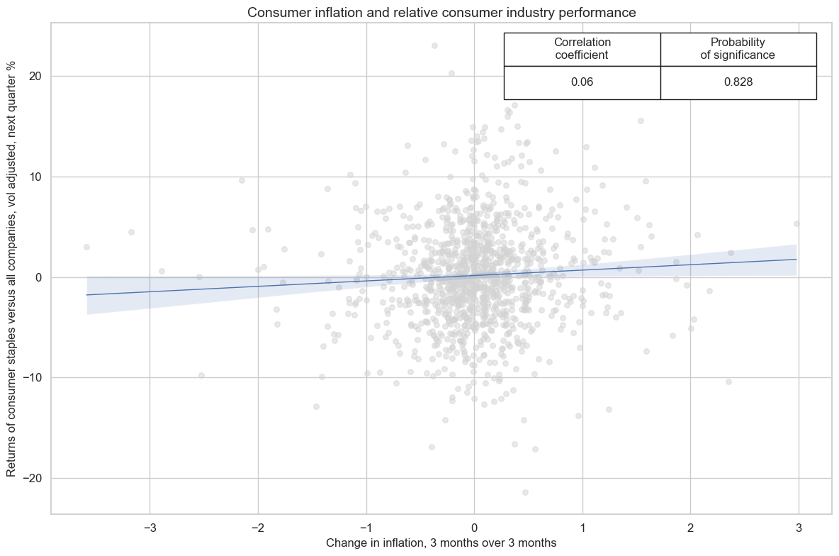
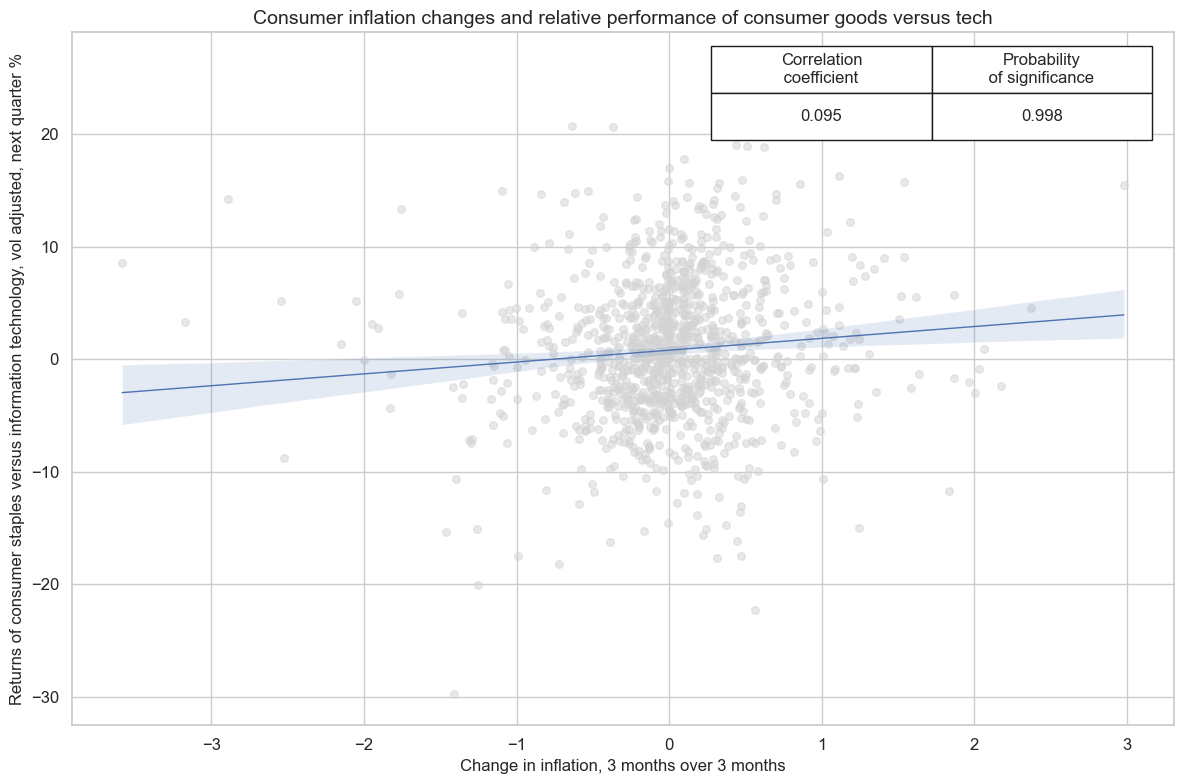
A rising consumer price inflation is usually conducive for higher interest rates and discount factors and, hence, tends to be negative for equity returns. However, for the consumer staples industry it also heralds higher nominal earnings. Hence, one should expect positive relative returns of consumer goods industries versus other sectors in general and against the IT sector in particular.

Empirical evidence supports these hypotheses. Signficance of consumer industries outperformance is not very high, however.

cidx = cids_exp
others = ['ALL', 'ITE', "UTL", "REL"]
formulas = [
    f"EQCCOSv{sector}R_VT10 = EQCCOSR_VT10 - EQC{sector}R_VT10" for sector in others
]

df_calc = msp.panel_calculator(df=dfd, calcs=formulas, cids=cidx)
dfd = msm.update_df(dfd, df_calc)

xcatx = ['CPIC_SA_P1M1ML12_D1M1ML3', "EQCCOSvALLR_VT10"]

rotation_cr = msp.CategoryRelations(
    dfd,
    xcats=xcatx,
    cids=cidx,
    freq="Q",
    lag=1,
    xcat_aggs=["last", "sum"],
    start=start_date,
)

rotation_cr.reg_scatter(
    title="Consumer inflation and relative consumer industry performance",
    labels=False,
    xlab="Change in inflation, 3 months over 3 months",
    ylab="Returns of consumer staples versus all companies, vol adjusted, next quarter %",
    coef_box="upper right",
    prob_est="map",
    fit_reg=True,
    reg_robust=False,
    single_chart=True,
)

CPIC_SA_P1M1ML12_D1M1ML3 misses: ['HKD'].

xcatx = ['CPIC_SA_P1M1ML12_D1M1ML3', "EQCCOSvITER_VT10"]

rotation_cr = msp.CategoryRelations(
    dfd,
    xcats=xcatx,
    cids=cidx,
    freq="Q",
    lag=1,
    xcat_aggs=["last", "sum"],
    start=start_date,
)

rotation_cr.reg_scatter(
    title="Consumer inflation changes and relative performance of consumer goods versus tech",
    labels=False,
    xlab="Change in inflation, 3 months over 3 months",
    ylab="Returns of consumer staples versus information technology, vol adjusted, next quarter %",
    coef_box="upper right",
    prob_est="map",
    fit_reg=True,
    reg_robust=False,
    single_chart=True,
)

CPIC_SA_P1M1ML12_D1M1ML3 misses: ['HKD'].

Appendices

Appendix 1: Sectoral equity index construction

The index is formed using stocks that are part of the universe in each region-sector at that point in time.

The universe selection happens on the basis of the the ranking of a company’s average market cap, measured in USD, over the last three months per the selection date of the universe. This universe is updated each month.

The index too is re-calculated on a monthly frequency, at the end of each month based on data known at or before the month end (the index selection date). The constituents are weighted by (current) market cap when the index is formed, and then the weights are allowed to float freely based on market movements between each rebalancing date.

Index positions are initiated on the first weekday occurring 4 calendars days after the index selection date and updated (i.e. performance and related data metrics) each weekday regardless of the date being a traded date for any/all of the issues in each index (the index calculation day).

Developed markets indices are formed using all stocks within the selected universe (more below in Appendix 2 ), regardless of the capitalisation.

On the other side, emerging market country indices have been limited to Large & Mid Caps only, which is reflected in the size of the corresponding macro-regions.

Appendix 2: Sectoral equity index specification

The geographical specification is two-tiered.

First the global set of stocks is split into six macro-regions, three for developed markets and three for emerging ones.

• Developed markets:

  • Americas: The largest 2250 issues of stocks with the issue country classification (the country) equal to either of (USA, CAN) and where the traded currency (the currency) being equal to either of (USD, CAD)

  • EMEA: The largest 1500 issues of stocks where the country is equal to either of (NLD, CHE, SWE, NOR, DEU, FIN, AUT, DNK, GBR, FRA, ESP, BEL, IRL, LUX, ITA, PRT, ISR) and where the currency equals either of (NLG, CHF, SEK, NOK, DEM, FIM, ATS, DKK, GBP, FRF, ESP, BEF, IEP, LUF, ITL, PTE, EUR, ILS)

  • Asia Pacific: The largest 1500 issues of stocks where the country is equal to either of (AUS, NZL, SGP, HKG, JPN) and where the currency is equal to either of (AUD, NZD, SGD, HKD, JPY)

• Emerging markets:

  • Americas: The largest 100 issues of stocks where the country is equal to either of (ARG, BRA, CHL, COL, MEX, PER)

  • EMEA: The largest 150 issues of stocks where the country is equal to either of (CZE, EGY, GRC, HUN, POL, QAT, SAU, ZAF, TUR, ARE, RUS)

  • Asia pacific: The largest 1000 issues of stocks where the country is equal to either of (CHN, IND, IDN, KOR, MYS, PAK, PHL, TWN, THA)

Then the single country indices are formed based on the subset of constituents available in the parent region:

• AUD: The subset of the DM Asia pacific eligible universe where the country equals AUS and the currency equals AUD

• BRL: The subset of the EM Americas eligible universe where the country equals BRA

• CAD: The subset of the DM Americas eligible universe where the country equals CAN and the currency equals CAD

• CHF: The subset of the DM EMEA eligible universe where the country equals CHE and the currency equals CHF

• CLP: The subset of the EM Americas eligible universe where the country equals CHL

• CNY: The subset of the EM Asia pacific eligible universe where the country equals CHN and the currency equals CNY

• COP: The subset of the EM Americas eligible universe where the country equals COL

• CZK: The subset of the EM EMEA eligible universe where the country equals CZE

• DEM: The subset of the DM EMEA eligible universe where the country equals DEU and the currency equals either of (EUR, DEM)

• EUR: The subset of the DM EMEA eligible universe where the country equals either of (NLD, DEU, FIN, AUT, FRA, ESP, BEL, IRL, LUX, ITA, PRT) and where the currency equals either of (NLG, DEM, FIM, ATS, FRF, ESP, BEF, IEP, LUF, ITL, PTE, EUR)

• ESP: The subset of the DM EMEA eligible universe where the country equals ESP and the currency equals either of (EUR, ESP)

• FRF: The subset of the DM EMEA eligible universe where the country equals FRA and the currency equals either of (EUR, FRF)

• GBP: The subset of the DM EMEA eligible universe where the country equals GBR and the currency equals GBP

• HUF: The subset of the EM EMEA eligible universe where the country equals HUN

• HKD: The subset of the DM sia pacific eligible universe where the country equals HKG and the currency equals HKD

• IDR: The subset of the EM Asia pacific eligible universe where the country equals IDN

• INR: The subset of the EM Asia pacific eligible universe where the country equals IND

• ITL: The subset of the DM EMEA eligible universe where the country equals ITA and where the currency equals either of (EUR, ITL)

• ILS: The subset of the DM EMEA eligible universe where the country equals ISR and where the currency equals ILS

• JPY: The subset of the DM sia pacific eligible universe where the country equals JPN and the currency equals JPY

• KRW: The subset of the EM Asia pacific eligible universe where the country equals KOR

• MXN: The subset of the EM Americas eligible universe where the country equals MEX

• MYR: The subset of the EM Asia pacific eligible universe where the country equals MYS

• NLG: The subset of the DM EMEA eligible universe where the country equals NLD and the currency equals either of (EUR, NLG)

• NOK: The subset of the DM EMEA eligible universe where the country equals NOR and the currency equals NOK

• NZD: The subset of the DM sia pacific eligible universe where the country equals NZL and the currency equals NZD

• PLN: The subset of the EM EMEA eligible universe where the country equals POL

• PEN: The subset of the EM Americas eligible universe where the country equals PER

• PHP: The subset of the EM Asia pacific eligible universe where the country equals PHL

• SGD: The subset of the DM sia pacific eligible universe where the country equals SGP and the currency equals SGD

• RUB: The subset of the EM EMEA eligible universe where the country equals RUS

• THB: The subset of the EM Asia pacific eligible universe where the country equals THA

• TRY: The subset of the EM EMEA eligible universe where the country equals TUR

• SEK: The subset of the DM EMEA eligible universe where the country equals SWE and the currency equals SEK

• TWD: The subset of the EM Asia pacific eligible universe where the country equals TWN

• USD: The subset of the DM Americas eligible universe where the country equals USA and the currency equals USD

• ZAR: The subset of the EM EMEA eligible universe where the country equals ZAF

The country codes refer to the ISO 3166-1 alpha-3 country code.

See Appendix 3 for the list of currency symbols used to represent each cross-section.

Appendix 3: Equity sector specification

The sector specification is part of the category definition. Stocks have been split into groups on the basis of their GICS classification:

• ALL: All GICS sectors

• COD: GICS Automobiles & Components, Consumer Durables & Apparel, Consumer Services and Retailing industry groups

• COS: GICS Food & Staples Retailing, Food, Beverage & Tobacco and Household & Personal Products industry groups

• CSR: GICS Telecommunication Services, and Media & Entertainment industry groups

• ENR: GICS Energy sector

• FIN: GICS Banks, Diversified Financials and Insurance industry groups

• HLC: GICS Health Care Equipment & Services and Pharmaceuticals, Biotechnology & Life Sciences industry groups

• IND: GICS Capital Goods, Commercial & Professional Services and Transportation industry groups

• ITE: GICS Software & Services, Technology Hardware & Equipment and Semiconductors & Semiconductor Equipment industry groups

• MAT: GICS Materials Sector

• REL: GICS Real Estate Industry Group

• UTL: GICS Utilities industry group

GICS sector specific indices are available only to DM countries.

Appendix 4: Currency symbols

The word ‘cross-section’ refers to currencies, currency areas or economic areas. In alphabetical order, these are AUD (Australian dollar), BRL (Brazilian real), CAD (Canadian dollar), CHF (Swiss franc), CLP (Chilean peso), CNY (Chinese yuan renminbi), COP (Colombian peso), CZK (Czech Republic koruna), DEM (German mark), ESP (Spanish peseta), EUR (Euro), FRF (French franc), GBP (British pound), HKD (Hong Kong dollar), HUF (Hungarian forint), IDR (Indonesian rupiah), ITL (Italian lira), JPY (Japanese yen), KRW (Korean won), MXN (Mexican peso), MYR (Malaysian ringgit), NLG (Dutch guilder), NOK (Norwegian krone), NZD (New Zealand dollar), PEN (Peruvian sol), PHP (Phillipine peso), PLN (Polish zloty), RON (Romanian leu), RUB (Russian ruble), SEK (Swedish krona), SGD (Singaporean dollar), THB (Thai baht), TRY (Turkish lira), TWD (Taiwanese dollar), USD (U.S. dollar), ZAR (South African rand).