Trend-following strategies exploit sustained past price movements, capitalizing on inefficiencies such as the gradual dissemination of information, inertia in portfolio reallocation, and disposition effects. However, the exclusive reliance on price data makes them highly sensitive to prevailing market regimes, neglects accompanying economic dynamics, and often leads to crowded positioning. These limitations can be mitigated by incorporating point-in-time information on concurrent macroeconomic trends.
We demonstrate the advantages of diversifying trend signals in the emerging-market FX space. While purely price-based strategies performed exceptionally during the EM boom and the global financial crisis of the 2000s, they struggled in the largely trendless markets of the 2010s and 2020s. By integrating macro support and headwind factors, one can construct macro-enhanced trends, i.e., signals that draw on a broader and more stable information set. Such approaches have delivered significantly higher risk-adjusted returns and sustained positive PnL even during periods of weak market trends.
The post below is based on Macrosynergy’s proprietary research. Please quote as “Cereda, Fabio and Sueppel, Ralph, ‘Diversified trend following in emerging FX markets,’ Macrosynergy research post, October 2025.” This post supersedes a previous article, “FX trend following and macro headwinds”.
A Jupyter notebook for auditing and replicating the research results is available for download here. The notebook operation requires access to J.P. Morgan DataQuery to download data from JPMaQS. Everyone with DataQuery access can download data except for the latest months. Moreover, J.P. Morgan offers free trials on the complete dataset for institutional clients. An academic support program sponsors data sets for research projects.
Market trend following and the benefits of macro information
Trend-following is an investment strategy that exploits the predictive power of sustained past market price movements or returns. It has been a popular trading principle for centuries. Its basis is the idea that markets revalue assets over extended periods, giving price trends a degree of persistence. Persistence can reflect gradual dissemination of information due, for example, to rational inattention (view post) or lazy trading (view post), herding, i.e., a conscious decision of investors to follow the crowd as opposed to their own analysis (view post), and the disposition effect of behavioral finance, investors’ tendency to sell positions that have been profitable and to hang on to those that have brought them losses (view post here).
Basic price-based trend-following strategies are inexpensive and straightforward to implement. They require only historical data and a live market price feed. No deep understanding of contract structures, valuation principles, or macroeconomic conditions is necessary. However, this very simplicity also entails important drawbacks:
- Seasonality means that the performance of trend following depends on the market regime. Price-based trend following provides good signals in extended periods of repricing but struggles when prices drift sideways or, worse, are range-bound. The example of emerging market currencies, illustrated below, shows that positive and negative seasons can last for a decade or longer.
- Macro headwinds are defined as economic developments that undermine prevailing medium-term market price trends. Large and persistent market repricing typically invites opposing macroeconomic developments over time. For example, the macro headwinds of a currency appreciation trend would include deteriorating external balances and economic performance. Conversely, a macro tailwind is a development that supports current market trends. Disregarding macro trends bears the risk of regular market excesses and setbacks.
- Crowded trades arise because the low information costs and widespread popularity of trend-following lead many investors to use similar parameters. As a result, trends can initially become self-reinforcing but eventually generate substantial endogenous market risk, i.e., uncertainty driven by the collective behavior of market participants. In this context, such risk manifests as setback risk: an asymmetry between downside and upside mark-to-market exposure caused by concentrated investor positioning (view summary).
Combining market trends with macro trends is a straightforward remedy to some of these faults. The incorporation of macro trends reduces the seasonality or regime-dependence of a standard trend following strategy because it adds an additional source of value generation. Monitoring macroeconomic developments that represent head- or tailwinds for macro trends also mitigates exposure to market excesses. Finally, point-in-time macro trends are not (yet) widely included in trend following systems and, thus, their consideration lessens the probability of playing in a crowded field. Overall, the diversification of trend principles should support consistency of value generation and reduce the incidence of large drawdowns.
Macro factors that enhance EMFX trend following
In this post, we illustrate the usefulness of complementary macro factors for emerging markets’ FX trend following. “Complementary” here means macro factors that provide evidence of macro headwinds or tailwinds for prevailing medium-term FX forward return trends. For statistical testing and PnL simulations, such factors must be calculated based on point-in-time information states of related indicators, also called “quantamental indicators”. These can be taken from the J.P. Morgan Macrosynergy Quantamental System (JPMaQS) for all major EM countries.
For emerging-market FX forward trend-following, we selected five complementary conceptual macro factors. Each is formulated as a theoretical positive driver of local-currency returns and computed without any form of optimization. The approach is intended as a proof of concept rather than a finalized or recommended strategy:
- External balance trends: These are sustained shifts in external balances as a ratio to GDP. Positive shifts towards smaller deficits or higher surpluses are indicative of improving competitiveness and decreasing external funding risks. The factor uses four indicators: merchandise trade balance and current account balance(seasonally adjusted) as % of GDP, latest 3 months versus 5-year average (documentation), merchandise trade balance as % of GDP, latest 3 months over the previous three months, and latest 6 months over the previous 6 months (documentation)
- International investment position improvements: These are positive shifts in the net international investment position of a country or reductions in international liabilities. Growing net assets or decreasing net liabilities reduce the risks of depreciation from disruptions in global capital flows. The factor averages six quantamental indicators: net international investment position as % of GDP, as change of the latest month over a year ago, change of the latest month over a 2-year moving average, and change of the latest month over a 5-year moving average (documentation), and international liabilities as % of GDP, as negative change of the latest month over a year ago, negative change of the latest month over a 2-year moving average, and negative change of the latest month over a 5-year moving average (documentation)
- Relative excess inflation rates: These are the differences in local CPI inflation rates versus the estimated effective local inflation target (documentation), expressed as a proportion of the effective local inflation target. Values are then measured relative to the benchmark currency area, e.g., the U.S. or the euro area (see details below). A relatively high deviation of CPI inflation from the local target should induce tighter monetary policy and greater tolerance for currency strength. Excess relative CPI inflation is calculated based on four CPI inflation indicators: annual headline consumer price inflation (documentation), headline CPI inflation % 6 months over the previous 6 months, seasonally- and jump-adjusted, and annualized (documentation), annual core CPI inflation (documentation), headline CPI inflation % 6 months over the previous 6 months, seasonally- and jump-adjusted, and annualized (documentation)
- Relative economic growth trends: These are nowcasted GDP growth differentials between the local emerging economy and the base currency area. High relative GDP growth indicates competitiveness and typically increases capital inflows and policymakers’ support for currency strength. The factor is calculated based on four point-in-time quantamental indicators: “intuitive” real GDP growth estimate, % over a year ago, and as a 3-month moving average, both outright and in excess of a five-year trailing median (documentation), and a “technical” real GDP growth estimate, % over a year ago, and as a 3-month moving average, both outright and in excess of a five-year trailing median (documentation).
- Excess export growth: This is the pace of merchandise export growth in local currency terms in excess of the effective local inflation target. High export growth points to a competitive manufacturing sector and strong local income generation, both of which support currency appreciation of smaller economies. The factor is calculated based on two macro-quantamental indicators: Merchandise exports in local currency, adjusted for seasonal effects, working days, as % of the latest 6 months over the previous 6 months at an annualized rate, and as % over a year ago, 3-month moving average (documentation).
Factors are calculated from indicators in a two-stage process. First, individual indicators are sequentially normalized around their theoretical neutral level, which here is always zero. The basis of normalization is the full panel of data, i.e., all country time series, up to the recorded point in time. Normalized scores are “winsorized”, i.e., floored or capped at three standard deviations in positive terms. The second step is a linear, equally weighted combination of all available indicator scores at each point in time. If one or the other indicator score is missing, the average is formed over the remaining ones. For details, see the attached Jupyter notebook.
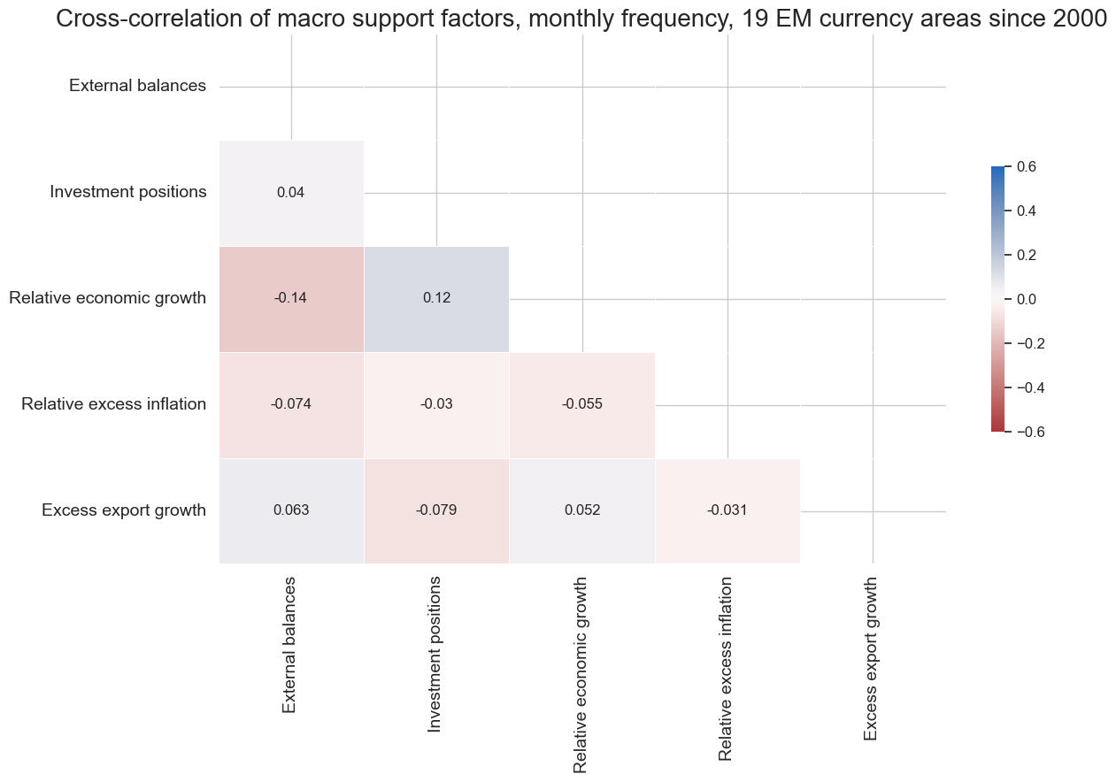
The correlation matrix below shows monthly cross-factor correlation coefficients based on the full panel of EM countries and observations since 2000. All correlation coefficients have been less than 15%, emphasizing that the chosen are not conceptually but also statistically distinct.
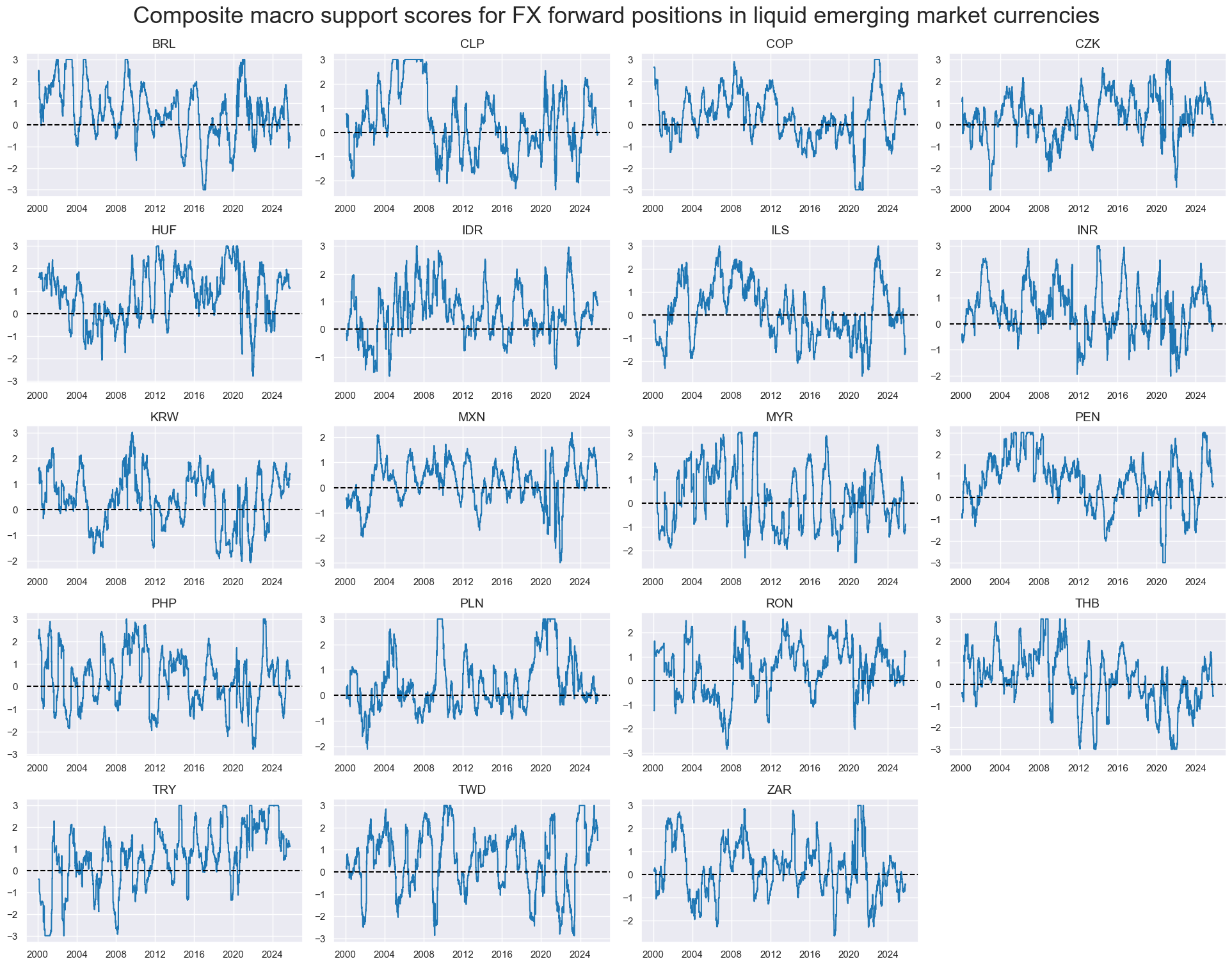
Finally, we re-normalize the conceptual factors and combine them into a single macro support score for each country. The line charts below illustrate the macro support scores across all emerging markets since 2000, showing medium-term dynamics, cyclical fluctuations, and some limited short-term volatility.
FX forward trend metrics
We calculate trend following signals for 1-month FX forward returns for a set of 19 emerging market currencies (documentation). This set includes all liquid EMFX markets for currencies with flexible exchange rates and a high degree of convertibility for at least part of the sample period 2000-2025. Periods of restricted tradability or exchange rate targeting are identified by using FX tradability and flexibility “dummies” of JPMaQS (documentation). The relevant EM and base currencies are:
- the Brazilian real (BRL), the Chilean peso (CLP), the Colombian peso (COP), the Indonesian rupiah (IDR), the Israeli shekel (ILS), the Indian rupee (INR), the Korean won (KRW), the Mexican peso (MXN), the Malaysian Ringgit (MYR), the Peruvian sol (PEN), the Philippine peso (PHP), the Thai baht (THB), the Taiwanese dollar (TWD) and the South African rand (ZAR), all against the U.S. dollar;
- the Czech koruna (CZK), the Hungarian forint (HUF), the Romanian leu (RON), and the Polish zloty (PLN), against the euro; and
- Turkish lira (TRY) against an equally weighted basket of dollar and euro.
As in previous posts, we use Tzotchev’s (2018) robust trend-following method (view paper) to estimate EM FX forward trends. The concept uses past average market returns divided by their estimated standard deviation (“t-statistics”) for various lookback horizons. These statistics indicate the probability of a past negative or positive return trend being significant. Furthermore, volatility-adjusted average returns can be translated into intuitive signals within a range of -1 to +1, by using the following formula:
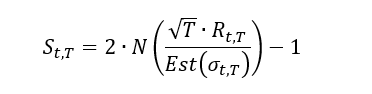
whereby
- St,T is a signal calculated at the end of day t based on a lookback period T,
- N is the cumulative distribution function for a normal distribution
- Rt,T is the average return at the end of day t over the lookback period T, and
- Est(σt,T) is the estimated standard deviation of the return over a lookback of T at the end of day t.
We consider two types of adjustments to this purely market price-based trend. Modification reduces or enhances the trend but does not override it by changing its sign. Balancing adds macro-quantamental information to the trend signal, giving them pre-assigned (here equal) weights, thus diversifying between market and macro trend signals.
Specifically, robust trend modification here is achieved by multiplying the original trend signal with a coefficient that can take values between 0 and 2, i.e., can reduce or double the original trend signal. That modification coefficient is a logistic (sigmoid) function of the macro support factor z-score.
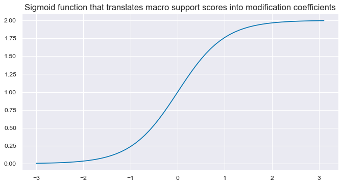
Specifically, the adjustment implements the following equation:
modified_trend = ((1 – sign(trend)) + sign(trend) * coef) * trend
for
coef = 2/(1 + exp(-2 * macroscore))
where trend means the original trend, sign() returns the sign of its element as 1/-1, and macroscore denotes the macro support score.
Note that modification depends on the sign of the concurrent trend signal: if the market trend signal is positive, a positive macro score enhances it, and a negative macro score reduces it. The logistic function translates the macro score such that for a value of zero, it is 1. For values of -1 and 1, it is 0.25 and 1.75, respectively, and for its minimum and maximum of -3 and 3, it is 0 and 2, respectively.
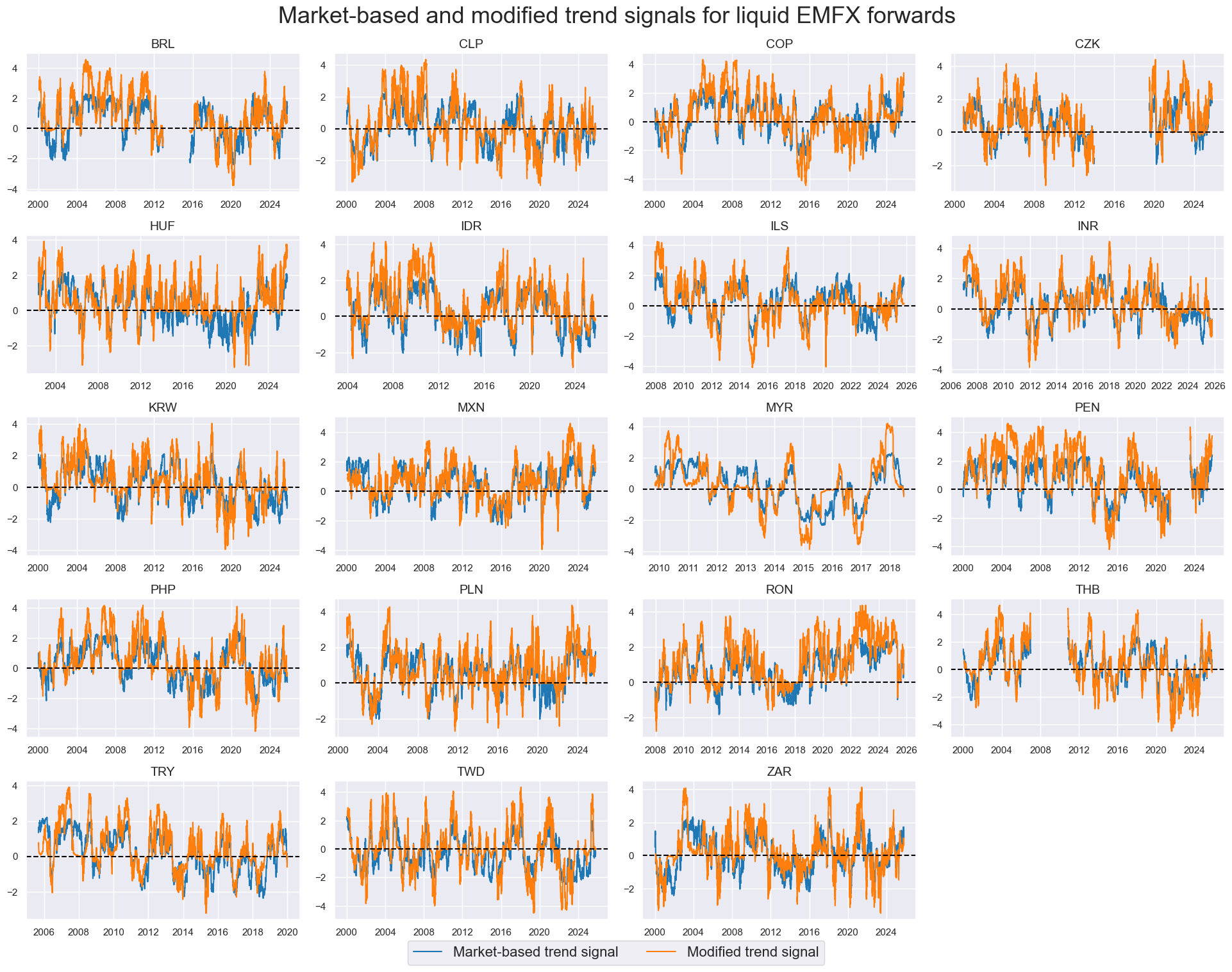
The line charts below compare robust trend signals and their modified values. While the signal signs are always equal, the values can be notably different. For example, positive market trends for short USDBRL positions in the second half of the 2000s were markedly enhanced by macro factors. In the case of short USDMXN positions in the2000s the market trend signals were usually reduced by macro factors.
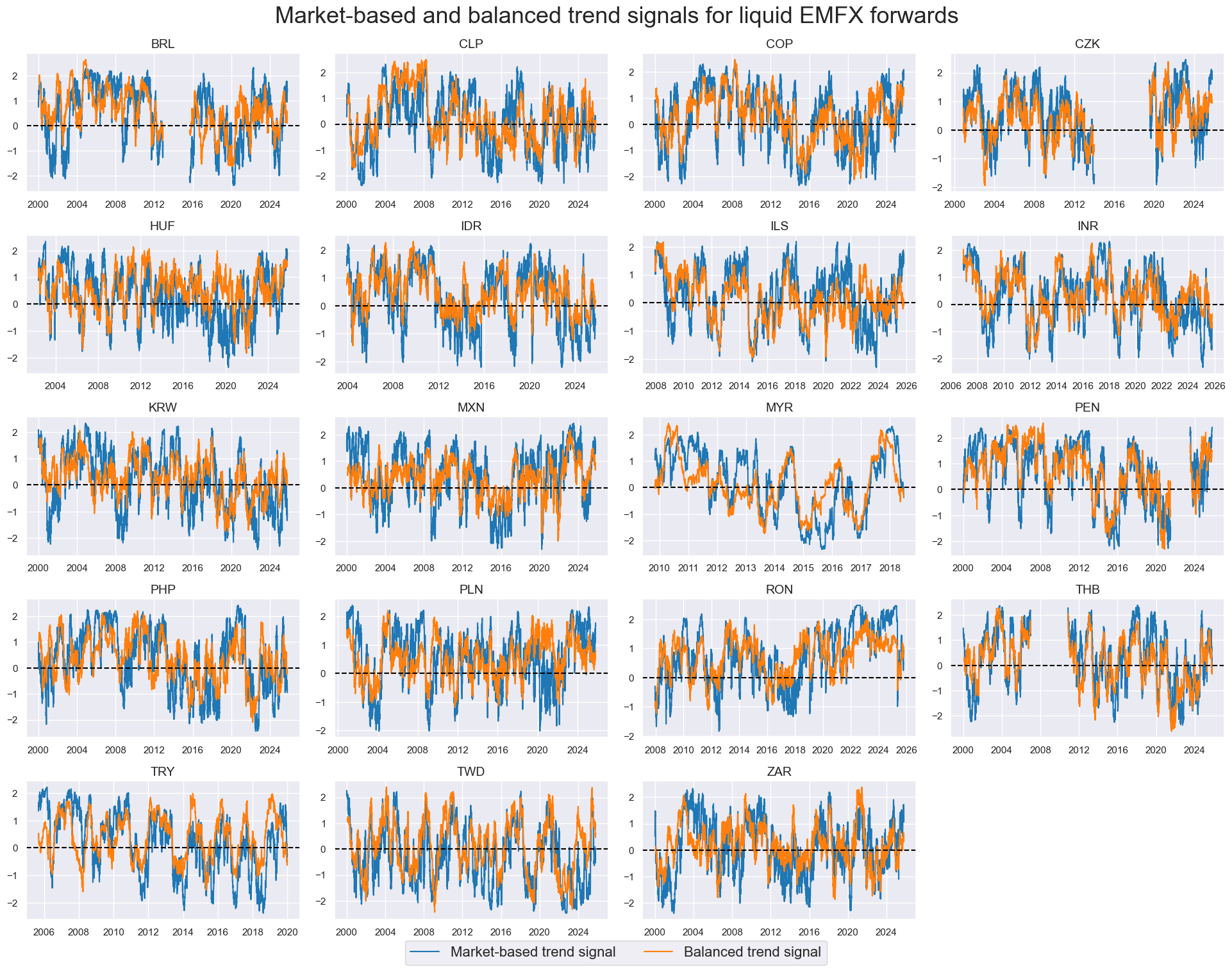
Rather than just modifying market trends, one can also use macro support factors to calculate “balanced trends”, i.e., signals that rely equally on the information of market return trends and point-in-time measures of macroeconomic trends. The balancing approach emphasizes the diversification of principles in signal generation. Previous posts have shown that market trends and macro trends have complementary strengths, with the former incorporating new information very swiftly (and cheaply) and the latter incorporating more in-depth and specific information (view post).
Here, we calculate a balanced trend as the average of a normalized robust trend score and the macro factor score. Unlike modified trends, balanced trends can have different signs from the original market-based trends. Generally, balancing changes the characteristics of the standard trend following strategy a bit more strongly than modification. The timelines of market-based trends and balanced trends below illustrate this.
Evidence of the benefits of diversified trend following
We empirically test whether modifying and balancing robust market trend signals in the EM FX forward space improves predictive power and PnL value generation. The basis of the evaluation is the application of these three types of signals to all tradable markets between 2000 and 2025 (October). The types of evaluation are predictive regressions, accuracy statistics, and naïve PnL simulations.
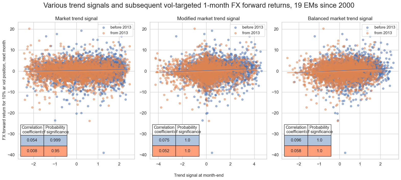
We investigate predictive power by means of panel regression analysis. This means we visualize and quantify the linear relation between the various trend signals and subsequent volatility-targeted FX forward returns across all 19 EM currency markets. A key metric is the significance of forward correlation, which requires a special panel test that adjusts the data of the predictive regression for common global influences across countries (view post here).
Here, we display scatter plots and one-month-ahead predictive correlation coefficients for panels of all 19 EM currency areas, separately for the first and second halves of the 26-year sample period. Forward correlation has been positive for all trend signals and all sample periods, and mostly with high statistical significance. However, forward correlation coefficients and probabilities of significance have been higher for the modified and balanced signals. The outperformance of these types of signals was particularly large in the second half of the sample period.
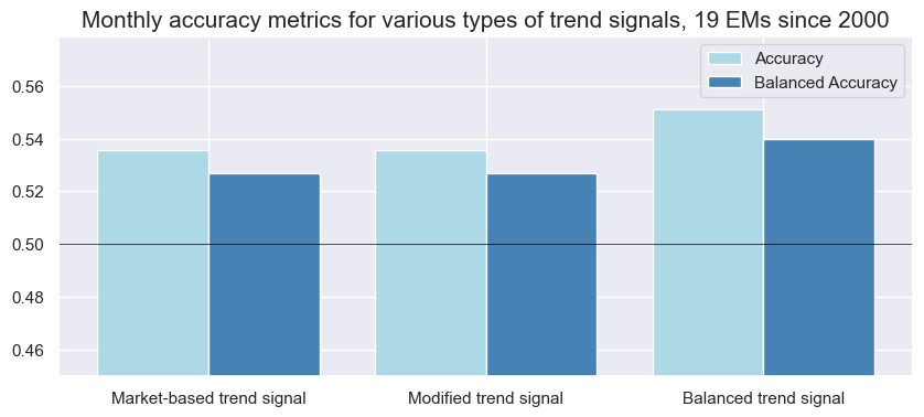
Accuracy measures a signal’s percentage of correctly predicted directions of subsequent returns. It not only shows an essential aspect of feature-target co-movement but also implicitly tests if the signal’s neutral (zero) level has been chosen appropriately. A critical metric for macro trading strategies is balanced accuracy, which averages the ratios of correctly predicted positive and negative returns, giving equal weight to a signal’s ability to predict both.
The monthly accuracy of the market-based robust trend signals has been 53.6% since 2000 for the full panel of tradable currency areas. Balanced accuracy was a bit lower at 52.7%. Due to the nature of adjustments, only balanced signals can have different accuracy values from standard market signals. Yet, the balanced trend’s signal accuracy was notably higher, with an overall monthly accuracy of 55.1% and balanced accuracy of 54.0%.
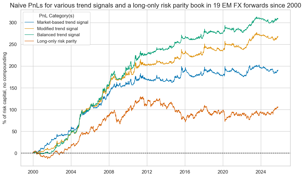
Finally, we assess the economic value of the various trend following signals by means of a naïve PnL simulation, in accordance with standard rules of the Macrosynergy posts. Naïve profit and loss series take positions in accordance with normalized signals and regular rebalancing. In the case of trend following, rebalancing is considered at a daily frequency, in accordance with signals at the end of the previous day, and allowing for a 1-day time-lapse for position adjustments. The trading signals need to be capped at a reasonable risk limit, which here has been set at three standard deviations on either the negative or positive side. Also, all positions are volatility targeted to avoid risk concentrations in the most volatile currencies and periods. A naïve PnL does not consider transaction costs or other risk management rules.
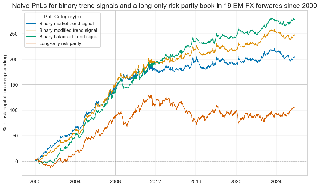
All trend following strategies outperformed a long-only (risk parity) EM FX forward portfolio since 2000. However, the standard market-based trend following strategy displayed extreme seasonality. After remarkable risk-adjusted returns in the 2000s, with Sharpe and Sortino ratios of 1.9 and 2.9, respectively, value generation almost ceased in the 2010s and 2020s, with Sharpe and Sortino ratios of 0.2 and 0.3. Roughly speaking, the market trend following strategy performed well when there was an actual strong return trend for the asset class and poorly when EMFX stopped trending.
The modified and, particularly, the balanced trend following signals reduced that seasonality and produced materially higher long-term value. The 26-year Sharpe and Sortino ratios of the market trend strategy were 0.7 and 1.0, respectively, with near-zero S&P500 correlation. The naïve PnL of the modified signals, which never changed the sign of position signals, already recorded higher ratios of 1.0 and 1.5. Meanwhile, the balanced trend following signal recorded a long-term Sharpe ratio of 1.2 and a Sortino ratio of 1.7, with less than 10% correlation with the S&P500 returns. Importantly, the balanced trend following signal continued to produce acceptable performance ratios also in the 2010s and 2020s, with an average Sharpe ratio of 0.7 and an average Sortino ratio of 1.0 before transaction costs.
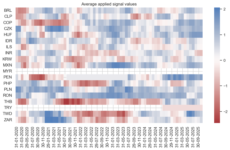
Although the trend-following strategy is rebalanced daily in principle, average daily trading volumes remain minimal due to the high autocorrelation of signals and the monthly frequency of volatility-targeting adjustments. The chart below illustrates the average monthly evolution of signals since 2020, underscoring this point. Long or short positions are typically maintained for three to six months, and in some cases, for several years.
However, one can make the strategy even more transaction cost-friendly by generating “binary signals” that primarily use the strength of trend metrics to manage position entry and exit barriers.
The below naïve PnL of a binary strategy uses the original signal and enters a long or short position if the signal value reaches one standard deviation. The position is kept, subject to vol-targeting adjustment, until the underlying signal falls below 0.25 standard deviation. Even for such binary strategies, the use of macro factors for modification and balancing has paid off handsomely, raising the long-term Sharpe and Sortino ratios from 0.8 and 1.1 for the market signal to 1.1 and 1.6, respectively, for the balanced signal.