Macro credit trades can be implemented through CDS indices. Due to obligors’ default option, long credit positions typically feature a positive mean and negative skew of returns. At the macro level, downside skew is reinforced by fragile liquidity and the potential for escalating credit crises. To enhance performance and create a chance to contain drawdowns, credit markets can be classified based on point-in-time macro factors, such as bank lending surveys, private credit dynamics, real estate price growth, business confidence dynamics, real interest rates, and credit spread dynamics. These factors support statistical learning processes that sequentially select and apply versions of four popular classification methods: naive Bayes, logistic regression, nearest neighbours, and random forest.
With only two decades and four liquid markets of CDS index trading, empirical results are still tentative. Yet they suggest that machine learning classification can detect the medium-term bias of returns and produce good monthly accuracy and balanced accuracy ratios. The random forest method stands out regarding predictive power and economic value generation.
Please quote as “Gholkar, Rushil and Sueppel, Ralph, ‘Classifying credit markets with macro factors,’ Macrosynergy research post, February 2025.”
A Jupyter notebook for audit and replication of the research results can be downloaded here. The notebook operation requires access to J.P. Morgan DataQuery to download data from JPMaQS. Everyone with DataQuery access can download data, except for the latest months. Moreover, J.P. Morgan offers free trials on the complete dataset for institutional clients. An academic support program sponsors data sets for research projects.
Macro credit risk
This post focuses on credit as a macro trade, i.e., on exposure to economy-wide default probabilities instead of exposure to a specific entity. Also, the intention is to take exposure to credit risk alone, as opposed to the term structure of risk-free interest rates. Corporate bonds typically depend on both. The closest tradable representation of macro credit risk positions are baskets or indices of credit default swaps (CDS). Generally, a single CDS is an over-the-counter derivative that provides insurance against the default of a specified entity. Being “long credit” through CDS markets means being a protection seller who receives periodic premia (CDS spreads) in exchange for compensation for default-related losses related to the specified obligor. No actual credit is being granted through this contract, but since it allows lenders to insure against default, credit conditions in the overall economy are still affected.
It is helpful to distinguish between default risk and credit risk:
- “A default risk is a possibility that a counterparty in a financial contract will not fulfil a contractual commitment… [By contrast] credit risk [is] risk associated with any kind of credit-linked events, such as changes in the credit quality (including downgrades or upgrades in credit ratings), variations of credit spreads, and the default event.” [Bielecki and Rutkowski]
- “Credit risk is defined as the degree of value fluctuations in debt instruments and derivatives due to changes in the underlying credit quality of borrowers and counterparties… Loss distributions are generally not symmetric. Since credit defaults or rating changes are not common events and since debt instruments have set payments that cap possible returns, the loss distribution is generally skewed toward zero with a long right-hand tail.” [Lopez and Saidenberg]
Indeed, insuring credit is akin to writing a call option on a borrower’s financial position. In the case of a corporation, the equivalent to the underlying price is the value of the creditor company, and the equivalent to the option’s strike price is the value of this company’s liabilities. When the liabilities of a company exceed its value, its shareholders should rationally opt to default. As Robert Merton pointed out in his seminal article on the pricing of corporate debt: “The [option pricing] approach could be applied to developing a pricing theory for corporate liabilities… The basic equation for the pricing of financial instruments is developed along Black-Scholes lines.”
At the macro level, default and credit risk can escalate into self-reinforcing crises. As credit risk increases, conditions for new credit deteriorate, and the resulting rise in borrowing costs makes defaults even more likely. Additionally, default risk in one sector of the economy can easily spread to banks, suppliers, and affiliated entities—a phenomenon often referred to as “contagion.” Containing such crises typically requires significant intervention by central banks and governments.
The nature and pricing of credit risk and limited liquidity in CDS markets suggest that the long-term distribution of macro credit risk returns has a positive mean with a negative skew. This means that long positions should post positive returns most of the time but large drawdowns in times of risk escalation.
CDS index markets
A CDS index is a derivative that gives exposure to the credit risk of a group of entities through a standardized basket of CDS. According to the main provider of these derivatives, IHS Markit, “a CDS index is an index whose underlying reference obligations are credit default swap instruments… CDS indices are among the most liquid instruments in the credit markets, enabling investors to efficiently access key market segments at low cost.” For the past two decades, the CDS index market has been dominated by two families of products. The CDX indices mainly cover North American entities, as well as emerging markets. The iTraxx indices focus more on Europe and Asia.
“Synthetic CDS indices originated in 2002 when JP Morgan launched the JECI and HYDI indices, which were later joined by Morgan Stanley’s Synthetic TRACERS. In 2003, both firms merged their indices to form the consolidated TRAC-X indices. During the same period, the index provider iBoxx also launched synthetic indices. While TRAC-X indices consisted of US names, iBoxx was active in the non-US credit derivatives market. In 2004, TRAC-X and iBoxx CDS indices merged to form the CDX indices in North America and the iTraxx indices in Europe and Asia. After being the administrator for CDX and calculation agent for iTraxx, IHS Markit (then ‘Markit’) acquired both families of indices in November 2007 and now owns the iTraxx and CDX indices, along with iTraxx SovX and MCDX Indices for derivatives and the iBoxx indices for cash bonds.” [IHS Markit]
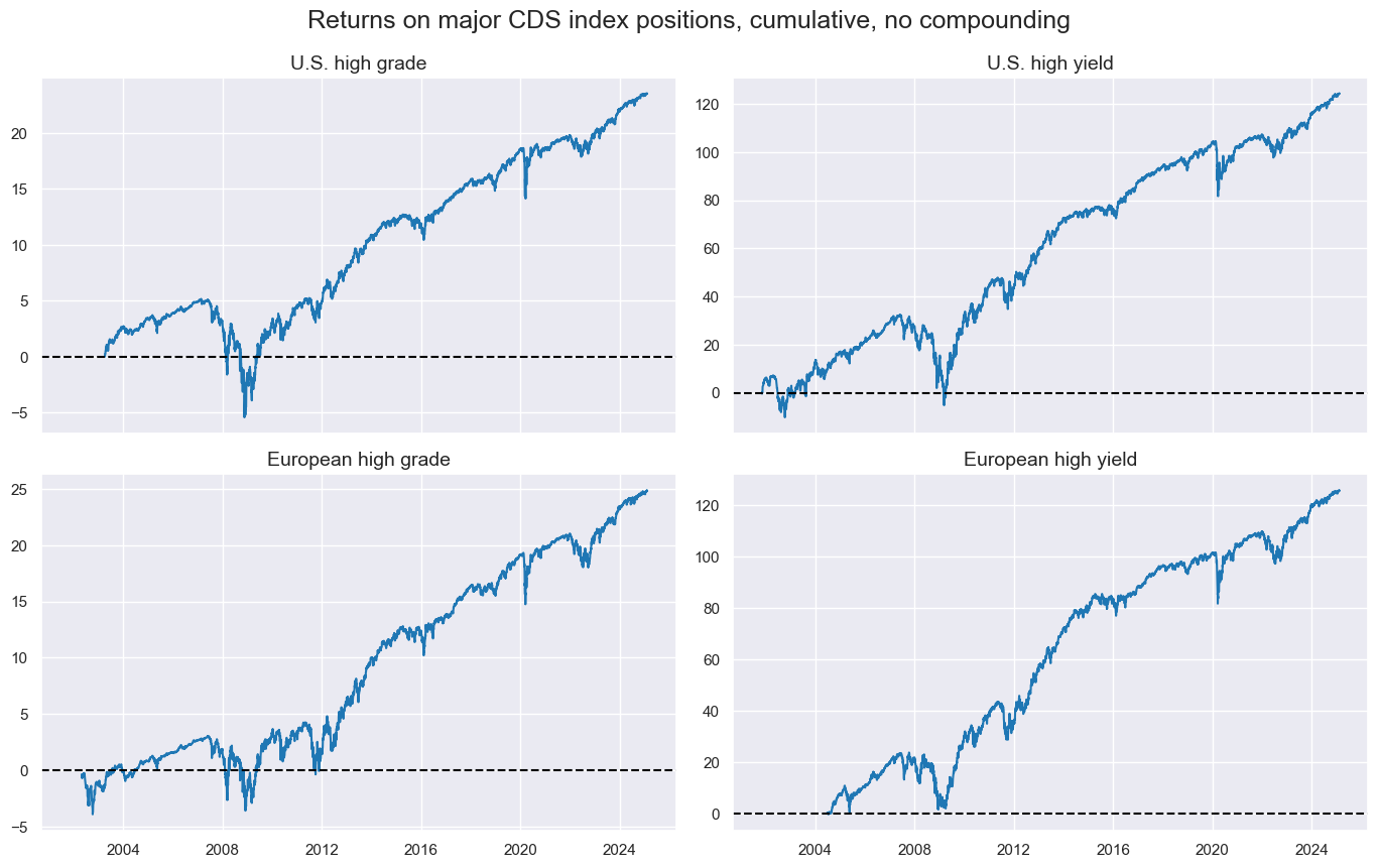
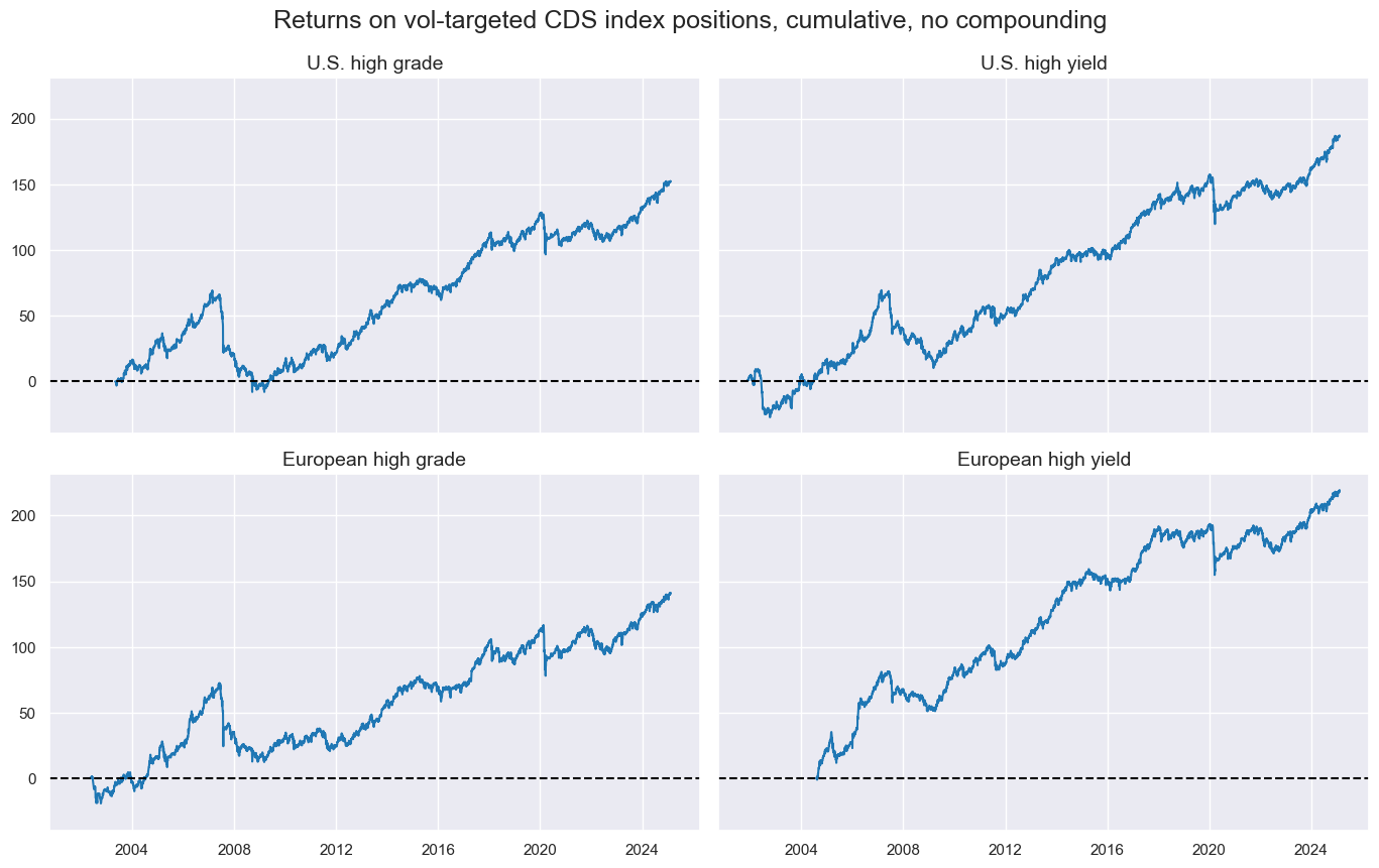
The empirical analysis in this post focuses on four popular contracts, two for the U.S. and two for Europe. These are the CDX U.S. investment grade index (UIG), the CDX U.S. high yield index (UHY), the iTraxx European investment grade index (EIG), and the iTraxx European crossover (high yield) index (EHY). A documentation of these indices can be found here. Generic returns for these have been taken as % of notional and for a 10% annualized volatility target from JPMaQS (view documentation).
Since inception, cumulative excess returns on these indices have displayed positive drifts, with occasional sharp drawdowns. Since 2002, the CDS index market has experienced one global systemic crisis (the Great Financial Crisis), one regional crisis (the euro area sovereign crisis), and one short-lived crash (related to the outbreak of the pandemic).
Vol-targeting, i.e., the scaling of positions across indices to a 10% annualized return standard deviation target, has reduced drawdowns in escalating crises but could not prevent sudden sharp drawdowns and also took a toll on post-crisis rebounds.
A macro-based classification strategy
The management of macro credit risk is challenging. The predominance and persistence of positive returns, i.e., the insurance premia for credit risk, discourages sustained short positions in active asset management. Meanwhile, the occasional appearance of credit crises threatens value preservation and the track record of active managers, particularly since the latter are easily stopped by escalating price dynamics and low liquidity. Trend following and volatility-targeting of credit derivatives positions can go some way in mitigating the effects of credit crises on portfolios. However, they fall short of information efficiency. None of these methods considers economic information related to the probability of an escalating crisis.
A natural enhancement of market timing strategies in credit markets is the consideration of macro factors that render negative returns more or less likely. In this post, we propose to do so through classification models that use relevant point-in-time macro information and that are trained and applied through sequential machine learning. The classification here is very simple, distinguishing merely between good and bad regimes for the credit market. A good regime is one where the expected credit return is positive. A bad regime is one where the expected credit return is negative. Since the former occurs more often than the latter, statistical learning is expected to set sufficiently high thresholds for short positions to render the overall strategy sustainable.
The main point of the macro credit classification approach is not to predict the inception of credit crises. These “trigger events” can come from many directions, such as political decisions and defaults of individual institutions and are hard to predict by macro information alone. However, macro-based classification offers two other benefits.
- Detecting escalation risk: Macro-quantamental indicators influence the probability of a credit crisis or recovery. For example, a confluence of rising credit spreads, deteriorating business sentiment, and obstacles to monetary policy support, such as inflationary pressure, would imply a high probability of self-reinforcing dynamics.
- Funding short positions: Not all negative returns in credit markets mark credit crises. There are occasional corrections without escalation potential, possibly reflecting monetary tightening, regulatory changes or modest economic downturns. Statistical learning with classification can detect these and thus build a rational basis for regular and affordable short positions.
For a meaningful analysis of the impact of economic conditions on credit markets, we use indicators of the J.P. Morgan Macrosynergy Quantamental System (“JPMaQS”). Quantamental indicators are point-in-time information states of the market and the public concerning meaningful economic indicators. They are suitable for testing predictive power and running backtesting related trading strategies. For this post, we use macro-quantamental indicators to represent six types of factors:
- Credit supply conditions: Credit supply conditions at banks affect companies’ access to funding and indicate the banks’ own funding position. We use loan supply condition scores of bank lending surveys and their seasonally adjusted changes, as 2-quarters over the previous two quarters (documentation here), as components of the factor.
- Private credit dynamics: This is another indicator of the availability of loans in the economy. A slowdown and contraction of private lending can indicate a credit crunch with increased risk to outstanding loans and bonds. The factor uses excess private credit growth, calculated as the difference between annual private credit growth (documentation here) and medium-term nominal GDP growth, and the change in annual credit growth (documentation here) over the past 12 months.
- Real estate price growth: With real estate being a major exposure and collateral of lenders, price dynamics in the sector should positively predict macro credit risk. The factor just takes an average between annual and 6 months over six months changes in residential real estate price growth (documentation here) relative to the effective inflation target of the central bank (documentation here).
- Business confidence dynamics: Changes in sentiment should plausibly reflect or predict changes in the financial position of companies, with a deterioration heralding rising credit risk. This factor is an average of short-term changes in seasonally adjusted business confidence in manufacturing (documentation here), construction (documentation here), and services (documentation here). The rates of change are three months over the previous three months and six months over the previous six months, all annualised.
- Expected real interest rates (negative): High real interest rates increase credit risk through their effects on funding costs and collateral valuation. The factor is based on 2-year and 5-year real interest rate swap rates (documentation here), subtracting either medium-term GDP growth or a constant. Then, we form an average and take the negative value.
- Credit spread dynamics (negative): Widening credit spreads imply tightening funding conditions and, hence, often indicate self-reinforcing dynamics. We calculate the proportionate widening of spreads in each of the four market segments (documentation here) based on two plausible measures: the change between the latest monthly average and the previous 3 months and the change between the latest 3 months and the previous six months. Both are divided by the base period spread to give a proportionate change.
Standard classification models for statistical learning
The objective is to classify the macroeconomic environment into favourable and unfavourable. Given the available history of credit derivative markets, this is a tall order for any classification method. Major credit indices return data are available from 2002-04. Since then, the world has experienced only two major macro credit crises, and only one of these has been truly global.
Here, statistical learning generates class predictions sequentially based on expanding time windows of “development data sets”. The process follows the basic principles explained in a previous post (“Optimizing macro trading signals – A practical introduction”).
- We specify model and hyperparameter grids containing all versions of a model type for predicting target returns based on factors. We do so separately for fundamentally different classification types to avoid excessive class variation from flipping between many different model versions over time.
- We set cross-validation parameters, i.e., rules for training and testing the different model versions within the development data sets. The main parameters are (1) the criterion according to which models are rated and (2) the cross-validation splitter that governs the partitions of the development data set into training and test sets. Here, the model evaluation criterion is the balanced accuracy score, and we use two different splitter types based on the Macrosynergy package classes ExpandingKFoldPanelSplit and RollingKFoldPanelSplit.
- Sequential hyperparameter selection and class predictions can be managed through the Macrosynergy package’s SignalOptimizer class. It uses scikit-learn model selection and cross-validation classes to produce return forecasts on monthly rebalancing dates, respecting the panel structure of the underlying data. Its calculate_predictions method governs the sequence of model selections, the optimal models’ parameter estimations, and the estimation of the classes.
We consider statistical learning processes with four types of classification models. The basic models are as follows.
Naïve Bayes classification
Naïve Bayes is a machine learning algorithm that categorizes items into predefined classes based on the historical probabilities of the feature values in an observed case occurring in a specific class. A naive Bayes classifier combines Bayes’ Theorem with the assumption that events are conditionally independent of each other. This makes the mathematics of classification easy and deals well with sparse data sets. However, it is a very strong assumption and explains why the method is called “naive.” The probability of a case belonging to a class can be calculated via Bayes’ rule:
P(y=i|X) = P(X|y=i) * P(y=i) / P(X)
where
- P(y=i|X) is the probability of the target variable (y) belonging to class i, given the observed feature set X,
- P(X|y=i) is the probability of the feature set X being observed when the target y belongs to class i,
- P(y=i) is the unconditional probability of the target variable y belonging to class i, and
- P(X) is the unconditional probability of the feature set X being observed.
The parameters of the probability functions are trained by maximizing the joint likelihood of target classes and features in the training sample. The assumption of events being independent makes the mathematics of classification easy and deals well with sparse data sets. However, in the case of credit returns and macro environment information states this is not the best approximation, as the macro information states are highly autocorrelated and cross-correlated.
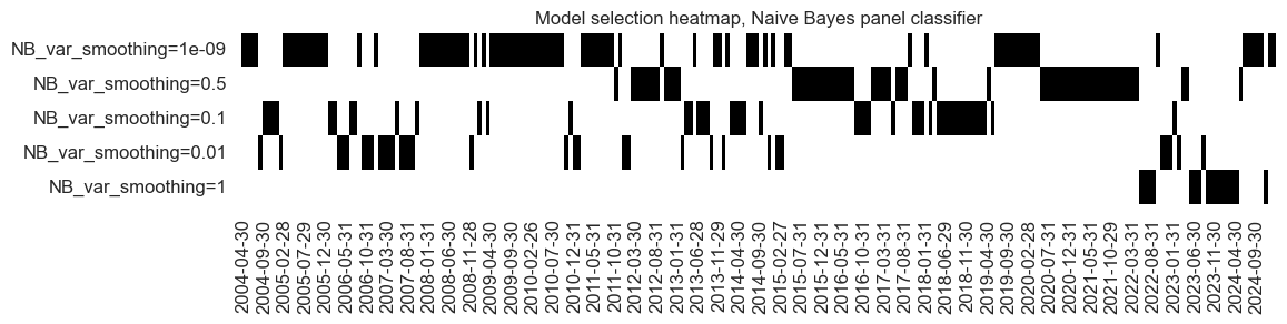
We implement Naïve Bayes by sequentially applying the GaussianNB class of the scikit-learn package to the expanding panel datasets. The only hyperparameter is variance smoothing the portion of the largest variance of all features that are added to variances for calculation stability, i.e., to prevent division by very small numbers. The hyperparameter has fluctuated over time and has failed to converge to date.
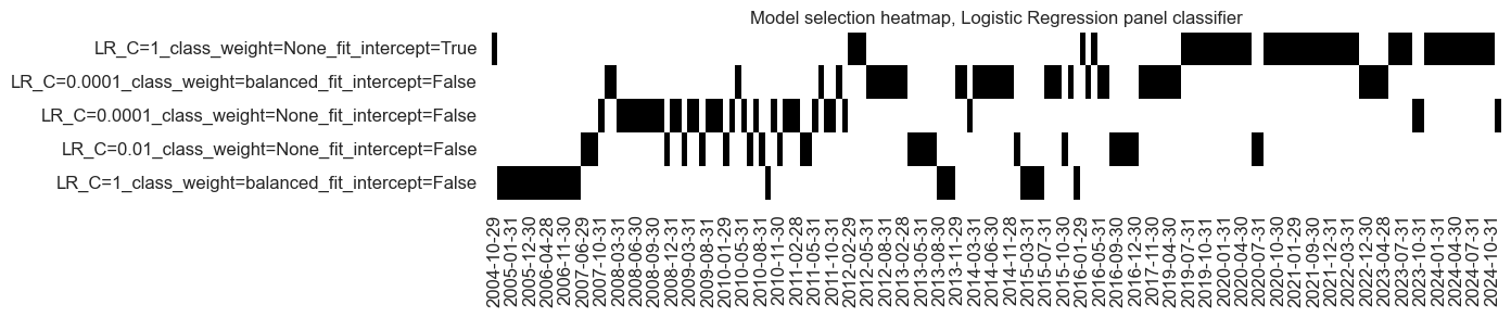
Logistic regression
Logistic regression is the classification counterpart of the linear regression model and uses the sigmoid function to transform a linear combination of inputs into a probability. Using a logistic function implicitly assumes a linear relationship between the features and the log odds of the positive class. The logistic regression becomes a classification method by setting a minimum probability threshold for positive classification, typically 50%.
A major limitation of this method is the implicit linear relation between macro environment variables and the odds ratios of the signs of credit returns. This obvious misspecification is plausibly a greater issue for credit than other markets due to the non-linear relation between credit returns and corporate asset values, as explained above.
We implement logistic regression for credit market classification by applying the LogisticRegression class of the scikit-learn package to the panel datasets. The hyperparameters are the inclusion of an intercept, which implies that neutral values of the factors are not really neutral, the class weight mode, which either gives all classes equal weight in the estimation or uses a balanced mode that weights inversely proportional to class frequency, and the regularization strength, i.e., the penalties imposed on large regression coefficients. There has been no clear model conversion over the sample period but a strong preference for the inclusion of the intercept and low regularization.
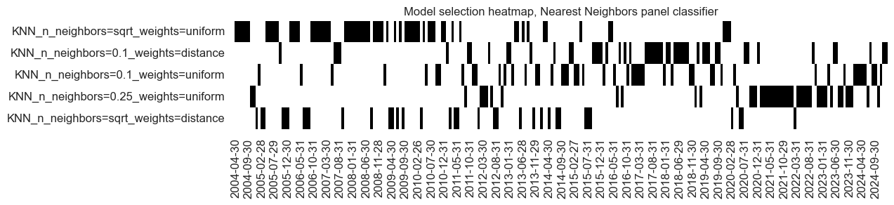
K-nearest neighbours classification
The K-nearest neighbours (KNN) algorithm is a particularly simple classification method. It uses a training set with known classifications and features (annotated observations) to predict the class of a new observation. The prediction is the class of the nearest annotated observations. The hyperparameter k gives the number of nearest neighbours considered. The value of k may be determined through hyperparameter tuning, but should also consider basic plausibility. For a small k, results can be distorted by outliers and are prone to instability. For a large k the method tends to simply allocated to the largest class. Like Naïve Bayes, KNN disregards temporal dependencies.
The neighbours’ classification has been implemented based on scikit-learn’s KNeighborsClassifier class. The main hyperparameters are the number of neighbours, here set as a share of the overall sample, and the weights applied to the neighbours for getting the class average, which can be either uniform or inverse to the distance of the predicted observation. There has been frequent model change over the past 20 years, but from late 2023, the learning process preferred a model with a small number of neighbours (10%) and uniform neighbour weights.
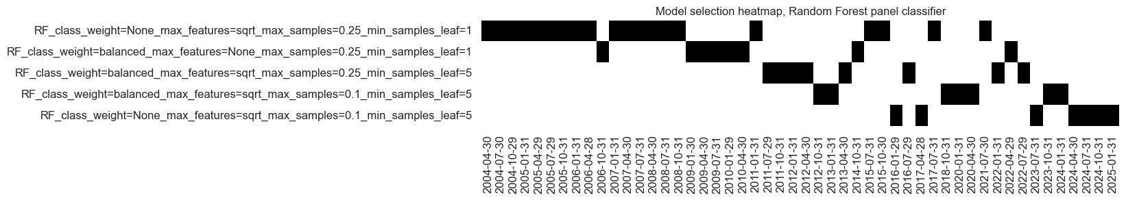
Random forest classification:
A Random Forest classifier is an ensemble machine learning algorithm that builds multiple decision trees and combines their predictions to improve accuracy and robustness. A decision tree formulates statements and makes decisions based on whether the statements are true or false. A decision tree that sorts into categories is a classification tree. Classification trees operate hierarchically from top to bottom until a classification is derived.
The top of a tree, i.e., the first statement to be evaluated, is called a root node. All lower evaluated statements are called internal nodes or branches. The ultimate classifications of the evaluations are called terminal nodes or leaves. The roots and internal nodes use feature values and thresholds to divide observations. The choice of features and threshold at each node is based on the predictive purity that is accomplished with respect to the targets. Pruning and minimum size requirements for leaves are critical to avoid overfitting. Exact parameters to that end can be derived through cross-validation.
Random forests seek a better bias-variance trade-off by harnessing a diversity of trees. Each tree is trained independently on a different “bootstrap sample” created by randomly drawing samples from an original dataset. Moreover, each node in a tree only considers a random subset of features for splitting the data. Classification returns the most frequent class predicted across trees.
The Random Forest classifier has been implemented through the RandomForestClassifier class of scikit-learn. The hyperparameters to be learnt are class weights, balancing classes or unweighted, the maximum ratio of features considered for a split and the maximum ratio of samples used for bootstrap. Model preference shifted as the sample expanded towards more diversity, i.e., smaller samples used for trees and a smaller number of considered features.
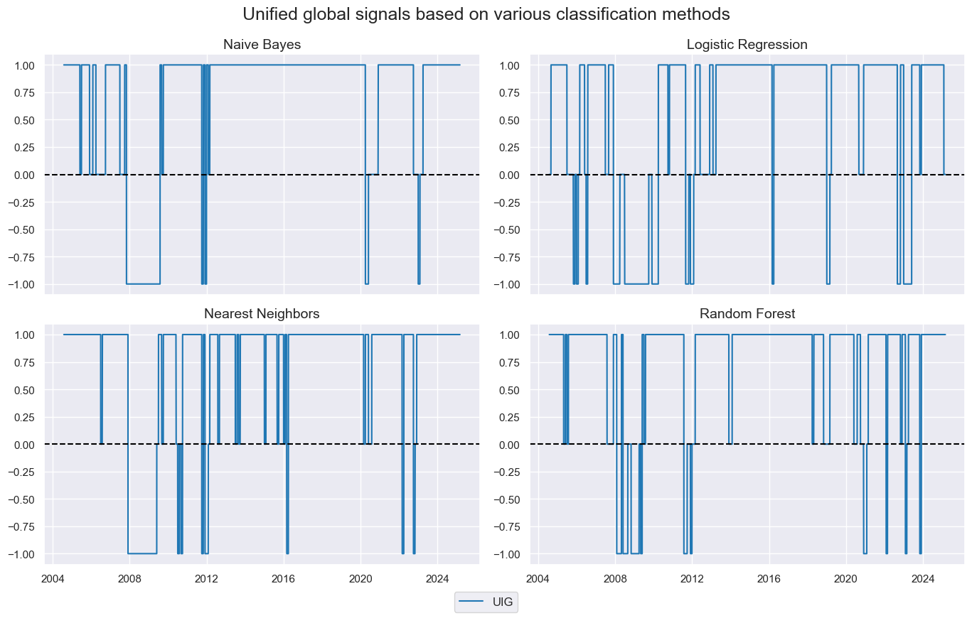
Each learning method is applied sequentially to expanding data sets of factors and subsequent returns for all four CDS index markets. This means it is based on expanding data panels, seeking to learn from global and market-specific experiences. While there is a common model applied to all markets, the differences in country- and market-specific parameters imply that, principally, the classes are estimated separately for each market. Classification results are naturally highly correlated across the four segments. However, they may occasionally differ, and to prevent class signals from producing relative cross-market trades, we calculated a single global signal by majority vote, with values of zero used when the vote is a tie. We call the results unified global signals.
Empirical results: the random forest supremacy
We evaluate the effectiveness of macro-based classification through accuracy statistics and various types of naïve backtested PnLs. This means that we test the out-of-sample forward classification success and economic value generation of the unified global signals.
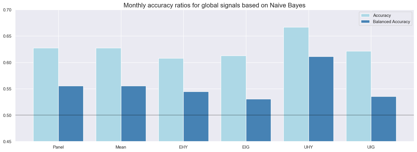
Monthly accuracy measures the ratio of correctly predicted signs of monthly returns based on the previous month’s signal. Balanced accuracy measures the average ratio of correctly predicted positive and negative monthly returns. The latter is more meaningful if the distribution of the return sign is temporarily unbalanced. In the case of CDS index returns since the early 2000s, about two-thirds of all monthly returns have been positive. Given the theory behind credit returns, this imbalance is likely to be a structural feature and, hence, both standard and balanced accuracy matter.
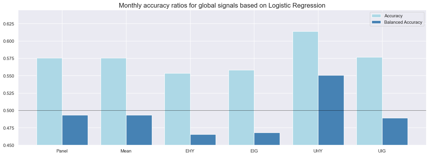
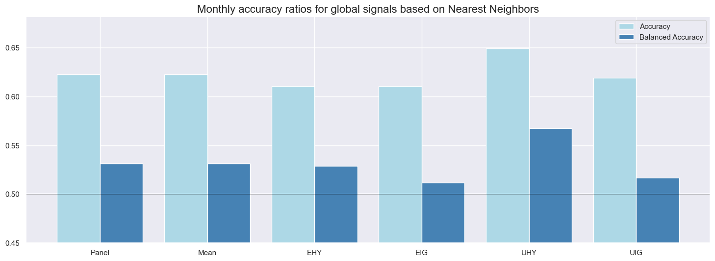
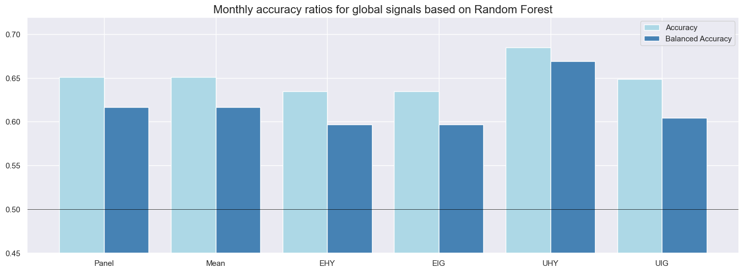
Average standard accuracy ratios at monthly frequency have been well above 50% for all classification methods. Across the panel of markets, the highest ratio (65%) was accomplished by the random forest model and the lowest (58%) by logistic regression. These high accuracy rates reflect a strong long bias in signals (between 81% and 91%), which afforded a high proportion of correctly predicted positive returns (62-66%) and, in conjunction with the predominance of positive returns, produced a high overall correct prediction rate. Note that the long bias in signals results from the learning process and has not been imposed by the methods or factors. By contrast, the specificity (proportion of correctly predicted negative returns) was mixed, between 35 and 58%, and only the random forest also did very well in predicting drawdowns.
Balanced accuracy has been between 49% and 62% for the full panel of markets. Again, the random forest method excelled, while logistic regression was the only method whose ratio slipped below 50%. Across markets, accuracy ratios were highest for the U.S. high-yield segment and lowest for European investment grade names, possibly reflecting differences in liquidity of the underlying CDS.
Naïve PnLs are calculated according to standardized rules across different Macrosynergy posts. Here, they use the unified global signals, which have values of -1, 0, and 1, at the end of each month as positioning signals for positions over the next month, subject to a one-day slippage for trading. The naïve PnLs do not consider transaction costs, risk management, or compounding.
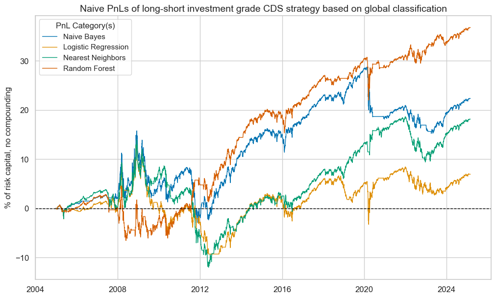
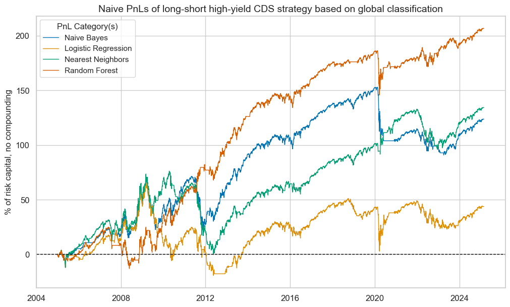
Long-short nominal CDS index PnLs
Here, the PnLs of the investment grade and high-yield segments should be viewed separately, as for similar positions, the high-yield portfolio PnL eclipses the investment-grade returns. We first look at conceptually balanced long-short strategies that simply take positions in accordance with the sign of the signal.
All classification methods have produced positive long-term PnLs for all market segments. However, differences in risk-adjusted returns were huge. The random forest signals produced long-term Sharpe ratios of 0.5-0.8 and Sortino ratios of 0.7-1.1, with S&P 500 correlation around 30%. The Naïve Bayes and nearest neighbours methods only recorded Sharpe ratios of 0.2-0.4 and Sortino ratios of 0.3-0.7, albeit with lower roughly 10-20% equity market correlation. The logistic regression signal only accumulated marginal risk-adjusted returns.
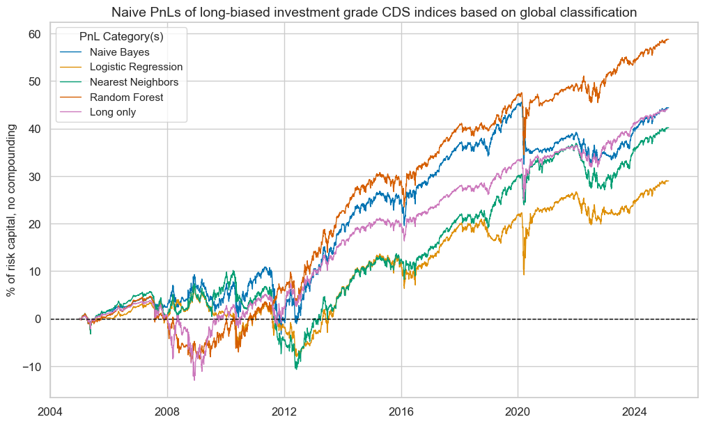
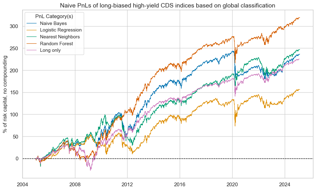
Long-biased nominal CDS index PnLs
A different way of looking at the value generated by classification signals is to add an explicit long bias and compare performance with a simple long-only portfolio. We introduce a long bias by adding a value of 0.5 to the unit signals, which means that positions will have notional amounts of -0.5 and 1.5 rather than -1 and 1. Then, we compare the PnL with a “long-only” book that always uses a positioning signal of 1.
Only the random forest classifier clearly outperformed the long-only PnL, both in terms of absolute and risk-adjusted returns. The naïve Bayes and nearest neighbours methods performed roughly at par with the long-only book, although with a lower correlation with the U.S. equity market. Logistic regression underperformed.
Most classification methods outperformed the “long-only” book during the great financial crisis, but none was any help during the outbreak of the COVID-19 pandemic. When drawdowns are unrelated to the macro factors we monitor, no classification method can prevent them.
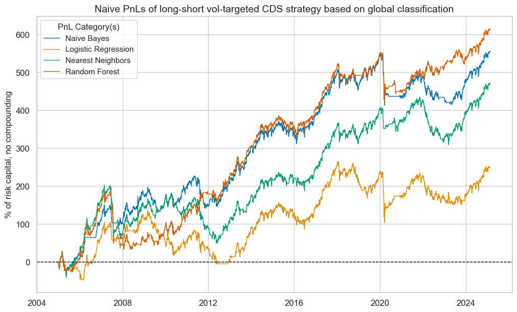
Long-short vol-targeted CDS index PnLs
Applying classification signals to volatility-targeted CDS index positions across market signals can facilitate risk management and increase long-term risk-adjusted returns. Here, this means that for each unit signal, we take a position with an expected annualized standard deviation of 10% of the risk capital based on lookback windows with exponentially decaying weights. Volatility targeting is not without drawbacks, however. In the case of sudden short-lived drawdowns the PnL suffers from the market decline and the increase in volatility at the same time while it does not receive the full benefit of the recovery if positions have been adjusted to increased volatility in the meantime. This has been exemplified by the behaviour of vol-targeted PnLs in the early months of the COVID-19 pandemic.
Over the past decades all classification strategies produced positive vol-targeted PnLs. The random forest and naïve Bayes methods recorded long-term Sharpe ratios of 0.7 and Sortino ratios of 0.9-1. The ratios for the nearest neighbours methods were slightly lower, and the logistic regression clearly underperformed.
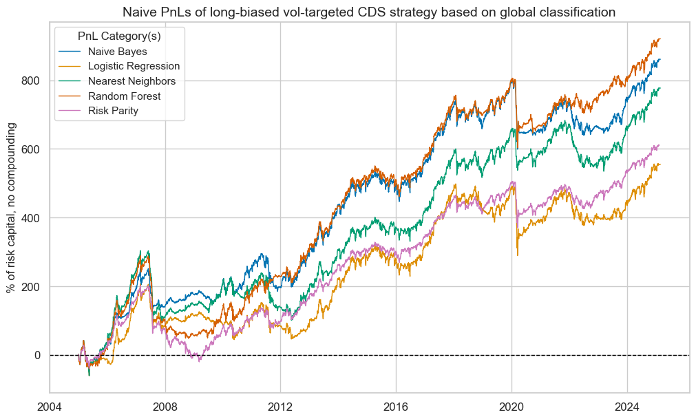
Long-biased vol-targeted CDS index PnLs
As before, we compare long-biased strategies based on the classification signals with a long-only book. However, here, long only also means volatility-targeted positions and hence, it is effectively a risk parity book across the four CDS indices.
Three of the four classification signals have outperformed the risk parity book over the past two decades. Again, the top performer has been the random forest classification, and the lowest risk-adjusted returns were recorded for the logistic regression method.