Classifying credit markets with macro factors #
Get packages and JPMaQS data #
import os
import numpy as np
import pandas as pd

from sklearn.pipeline import Pipeline
from sklearn.linear_model import LogisticRegression
from sklearn.ensemble import RandomForestClassifier
from sklearn.naive_bayes import GaussianNB

from sklearn.metrics import make_scorer, balanced_accuracy_score

import macrosynergy.management as msm
import macrosynergy.panel as msp
import macrosynergy.pnl as msn
import macrosynergy.signal as mss
import macrosynergy.learning as msl
import macrosynergy.visuals as msv

from macrosynergy.download import JPMaQSDownload

import warnings

warnings.simplefilter("ignore")
# Cross-sections
cids_dm = ["USD", "EUR"]
cids_ig = ["UIG", "EIG"]
cids_hy = ["UHY", "EHY"]
cids_cr = ["UIG", "UHY", "EIG", "EHY"]

cids = cids_cr + cids_dm
# Indicator categories
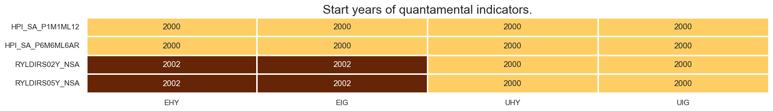
rates = [
"RYLDIRS02Y_NSA",
"RYLDIRS05Y_NSA",
]
hpi = [
"HPI_SA_P6M6ML6AR",
"HPI_SA_P2Q2QL2AR",
"HPI_SA_P1M1ML12",
"HPI_SA_P1Q1QL4",
]
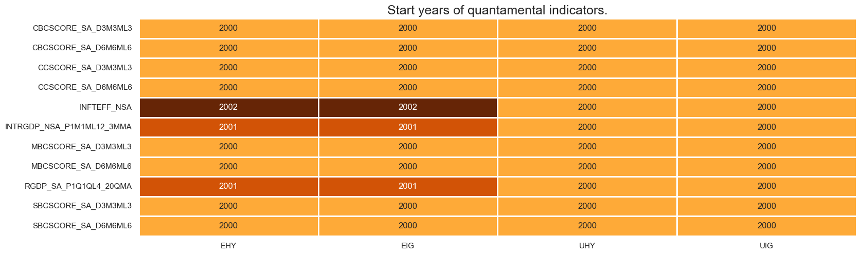
bsurv_changes = [
# Construction confidence
"CBCSCORE_SA_D6M6ML6",
"CBCSCORE_SA_D3M3ML3",
# Manufacturing confidence
"MBCSCORE_SA_D6M6ML6",
"MBCSCORE_SA_D3M3ML3",
# Services confidence
"SBCSCORE_SA_D6M6ML6",
"SBCSCORE_SA_D3M3ML3",
]
csurv_changes = [
"CCSCORE_SA_D6M6ML6",
"CCSCORE_SA_D3M3ML3",
]
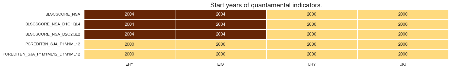
bank_lending = [
"BLSCSCORE_NSA",
"BLSCSCORE_NSA_D2Q2QL2",
"BLSCSCORE_NSA_D1Q1QL4",
]
credit = [
"PCREDITBN_SJA_P1M1ML12",
"PCREDITBN_SJA_P1M1ML12_D1M1ML12",
]
main = rates + hpi + bsurv_changes + csurv_changes + bank_lending + credit
econ = [
"INFTEFF_NSA",
"INTRGDP_NSA_P1M1ML12_3MMA",
"RGDP_SA_P1Q1QL4_20QMA",
]
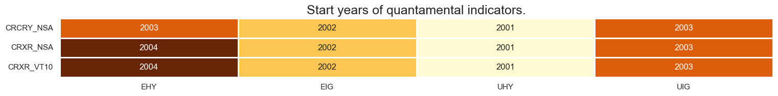
mark = [
"CRXR_VT10",
"CRXR_NSA",
"CRCRY_NSA",
]
xcats = main + econ + mark
# Tickers for download

single_tix = ["USD_GB10YXR_NSA", "USD_EQXR_NSA"]
tickers = (
    [cid + "_" + xcat for cid in cids_dm for xcat in main + econ]
    + [cid + "_" + xcat for cid in cids_cr for xcat in mark]
    + single_tix
)
# Download series from J.P. Morgan DataQuery by tickers

start_date = "2000-01-01"
end_date = None

# Retrieve credentials

oauth_id = os.getenv("DQ_CLIENT_ID")  # Replace with own client ID
oauth_secret = os.getenv("DQ_CLIENT_SECRET")  # Replace with own secret

# Download from DataQuery

downloader = JPMaQSDownload(client_id=oauth_id, client_secret=oauth_secret)
df = downloader.download(
    tickers=tickers,
    start_date=start_date,
    end_date=end_date,
    metrics=["value"],
    suppress_warning=True,
    show_progress=True,
)

dfd = df.copy()
dfd.info()
Downloading data from JPMaQS.
Timestamp UTC:  2025-02-14 15:28:31
Connection successful!
Requesting data: 100%|███████████████████████████████████████████████████████████████████| 3/3 [00:00<00:00,  4.66it/s]
Downloading data: 100%|██████████████████████████████████████████████████████████████████| 3/3 [00:17<00:00,  5.93s/it]
Some expressions are missing from the downloaded data. Check logger output for complete list.
4 out of 58 expressions are missing. To download the catalogue of all available expressions and filter the unavailable expressions, set `get_catalogue=True` in the call to `JPMaQSDownload.download()`.
Some dates are missing from the downloaded data.
2 out of 6557 dates are missing.
<class 'pandas.core.frame.DataFrame'>
RangeIndex: 338824 entries, 0 to 338823
Data columns (total 4 columns):
 #   Column     Non-Null Count   Dtype
---  ------     --------------   -----
 0   real_date  338824 non-null  datetime64[ns]
 1   cid        338824 non-null  object
 2   xcat       338824 non-null  object
 3   value      338824 non-null  float64
dtypes: datetime64[ns](1), float64(1), object(2)
memory usage: 10.3+ MB
Availability #
Renaming #
# Rename quarterly tickers to roughly equivalent monthly tickers

dict_repl = {
    "HPI_SA_P1Q1QL4": "HPI_SA_P1M1ML12",
    "HPI_SA_P2Q2QL2AR": "HPI_SA_P6M6ML6AR",
}

for key, value in dict_repl.items():
    dfd["xcat"] = dfd["xcat"].str.replace(key, value)
# Rename and duplicate economic area tickers in accordance with credit market tickers

dfa = dfd[
    (dfd["cid"].isin(["EUR", "USD"])) & ~(dfd["xcat"].isin(["EQXR_NSA", "GB10YXR_NSA"]))
]

dfa_ig = dfa.replace({"^EUR": "EIG", "^USD": "UIG"}, regex=True)
dfa_hy = dfa.replace({"^EUR": "EHY", "^USD": "UHY"}, regex=True)

dfx = pd.concat([dfd, dfa_ig, dfa_hy])
Check availability #
xcatx = rates + hpi
cidx = cids_cr

msm.check_availability(df=dfx, xcats=xcatx, cids=cidx, missing_recent=False)
xcatx = bsurv_changes + csurv_changes + econ
cidx = cids_cr

msm.check_availability(df=dfx, xcats=xcatx, cids=cidx, missing_recent=False)
xcatx = bank_lending + credit
cidx = cids_cr

msm.check_availability(df=dfx, xcats=xcatx, cids=cidx, missing_recent=False)
xcatx = mark
cidx = cids_cr

msm.check_availability(df=dfx, xcats=xcatx, cids=cidx, missing_recent=False)
Factor computation and checks #
Single-concept calculations #
factors = []
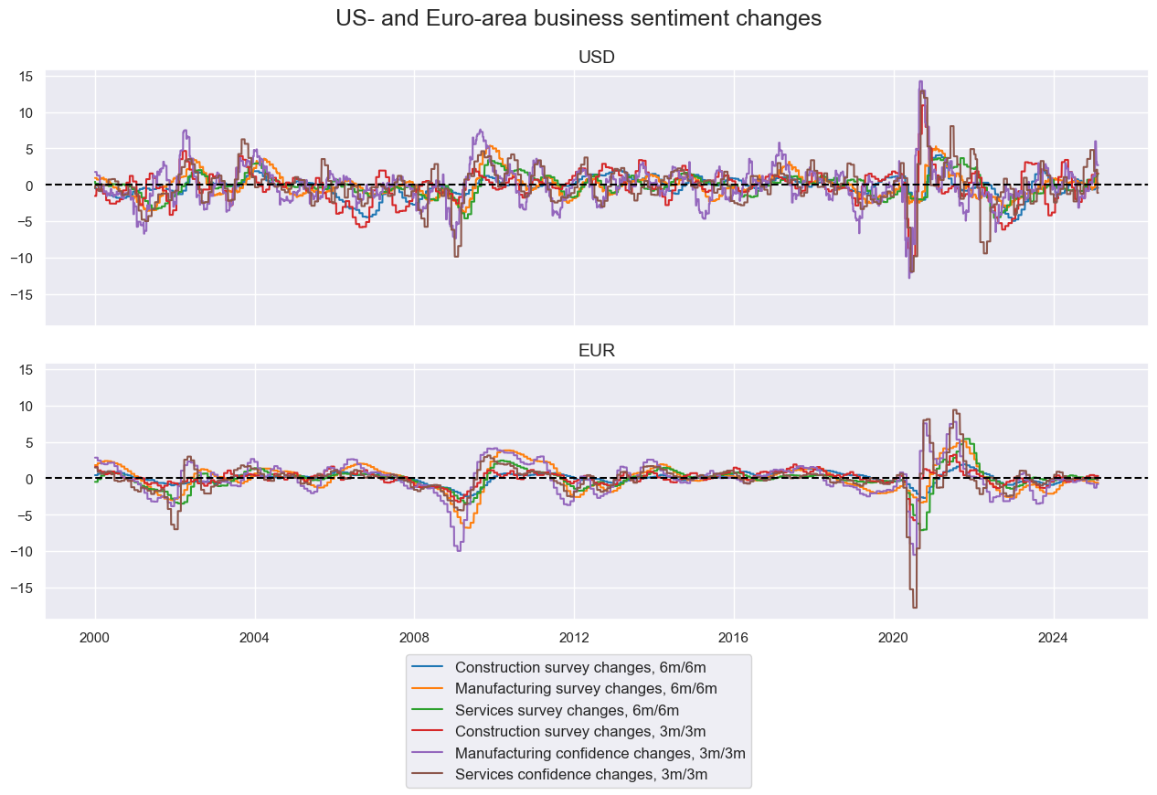
Business sentiment dynamics #
# Annualize sentiment score changes

cidx = cids_cr
calcs = []

bss = ["CBCSCORE_SA", "MBCSCORE_SA", "SBCSCORE_SA"]
for bs in bss:
    calcs.append(f"{bs}_D6M6ML6AR = {bs}_D6M6ML6 * 2")
    calcs.append(f"{bs}_D3M3ML3AR = {bs}_D3M3ML3 * 4")

dfa = msp.panel_calculator(df=dfx, calcs=calcs, cids=cidx)
dfx = msm.update_df(dfx, dfa)

bsar = [f"{bs}_D6M6ML6AR" for bs in bss] + [f"{bs}_D3M3ML3AR" for bs in bss]
cidx = ["UIG", "EIG"]
xcatx = bsar

msp.view_timelines(
    df=dfx,
    xcats=xcatx,
    cids=cidx,
    ncol=1,
    same_y=True,
    aspect=3,
    title="US- and Euro-area business sentiment changes",
    xcat_labels=[
        "Construction survey changes, 6m/6m",
        "Manufacturing survey changes, 6m/6m",
        "Services survey changes, 6m/6m",
        "Construction survey changes, 3m/3m",
        "Manufacturing confidence changes, 3m/3m",
        "Services confidence changes, 3m/3m",
    ],
    cid_labels=["USD", "EUR"],
)
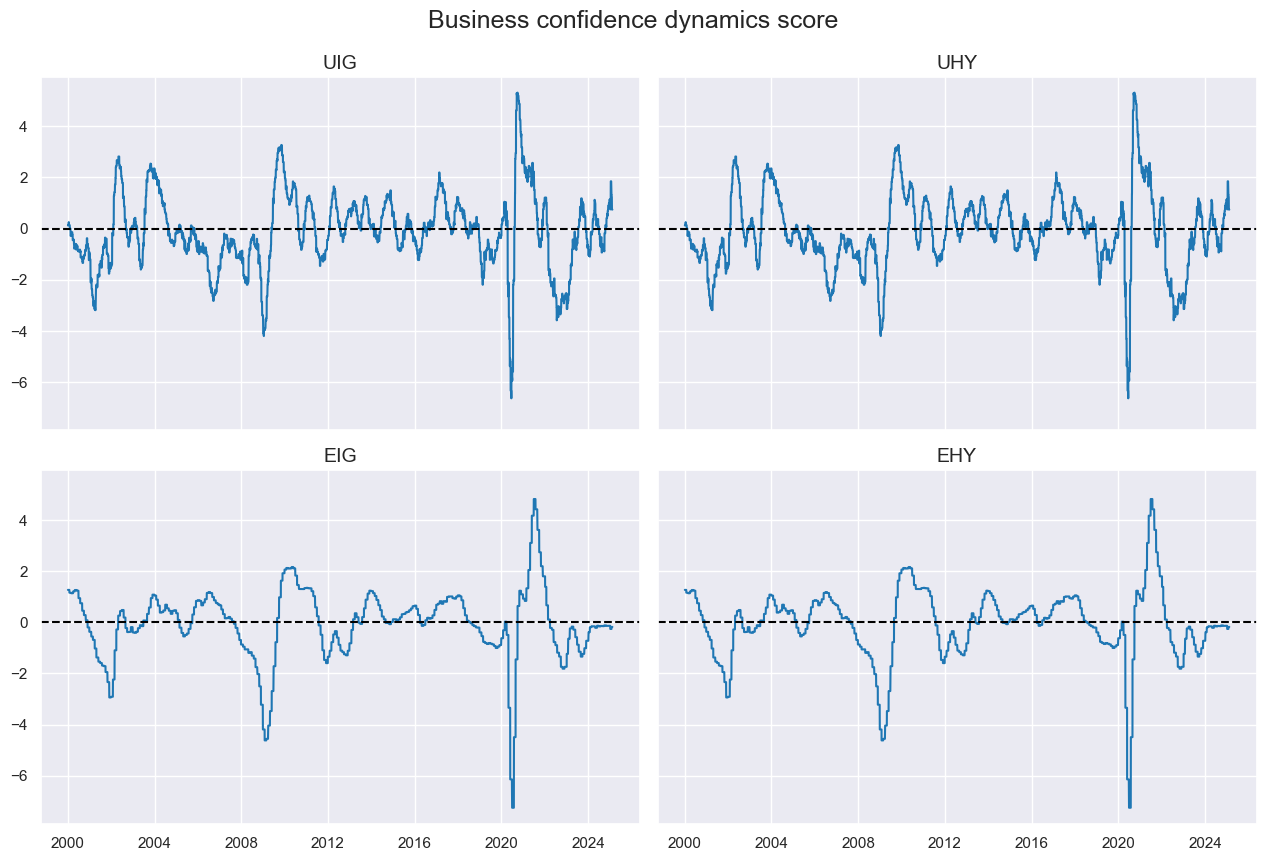
# Single business sentiment change
cidx = cids_cr
xcatx = bsar

dfa = msp.linear_composite(df=dfx, xcats=xcatx, cids=cids_cr, new_xcat="BCONFCHG")
dfx = msm.update_df(dfx, dfa)
cidx = cids_cr
xcatx = ["BCONFCHG"]

msp.view_timelines(
    df=dfx,
    xcats=xcatx,
    cids=cidx,
    title="Business confidence dynamics score",
    ncol=2,
    same_y=True,
    aspect=1.5,
)
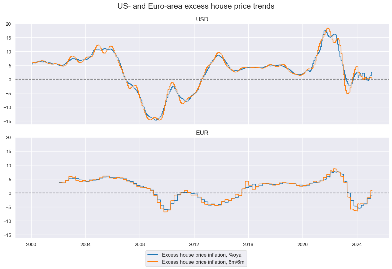
Excess house price trends #
# Excess house price growth

cidx = cids_cr
calcs = []

calcs.append(f"XHPI_SA_P1M1ML12 = HPI_SA_P1M1ML12 - INFTEFF_NSA")
calcs.append(f"XHPI_SA_P6M6ML6AR = HPI_SA_P6M6ML6AR - INFTEFF_NSA")

dfa = msp.panel_calculator(df=dfx, calcs=calcs, cids=cidx)
dfx = msm.update_df(dfx, dfa)

xhpi = ["XHPI_SA_P1M1ML12", "XHPI_SA_P6M6ML6AR"]
cidx = ["UIG", "EIG"]
xcatx = xhpi

msp.view_timelines(
    df=dfx,
    xcats=xcatx,
    cids=cidx,
    title="US- and Euro-area excess house price trends",
    ncol=1,
    same_y=True,
    aspect=3,
    xcat_labels=[
        "Excess house price inflation, %oya",
        "Excess house price inflation, 6m/6m",
    ],
    cid_labels=["USD", "EUR"],
)
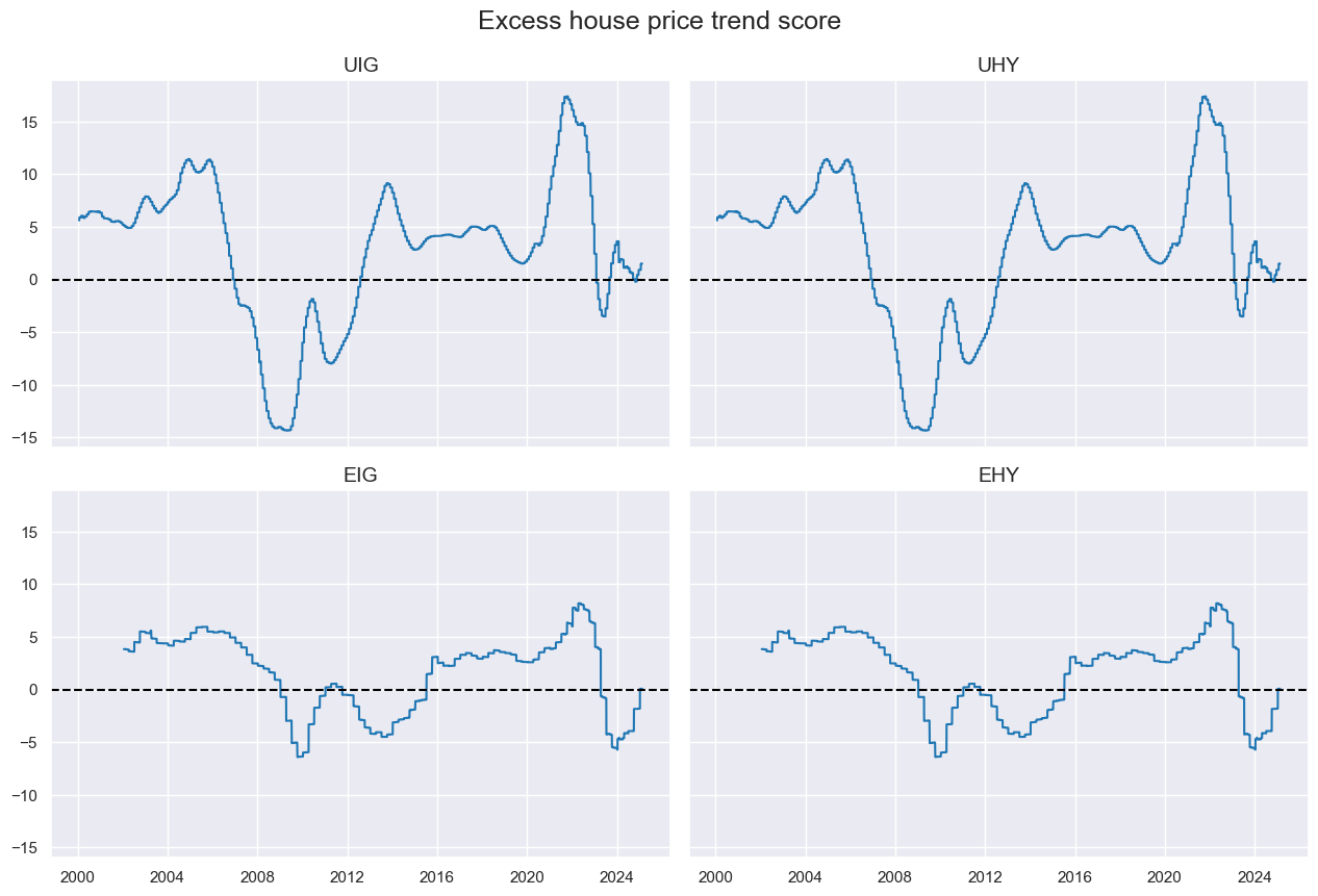
xcatx = xhpi
cidx = cids_cr

dfa = msp.linear_composite(df=dfx, xcats=xcatx, cids=cidx, new_xcat="XHPI")
dfx = msm.update_df(dfx, dfa)
cidx = cids_cr
xcatx = ["XHPI"]

msp.view_timelines(
    df=dfx,
    xcats=xcatx,
    cids=cidx,
    title="Excess house price trend score",
    ncol=2,
    same_y=True,
    aspect=1.5,
)
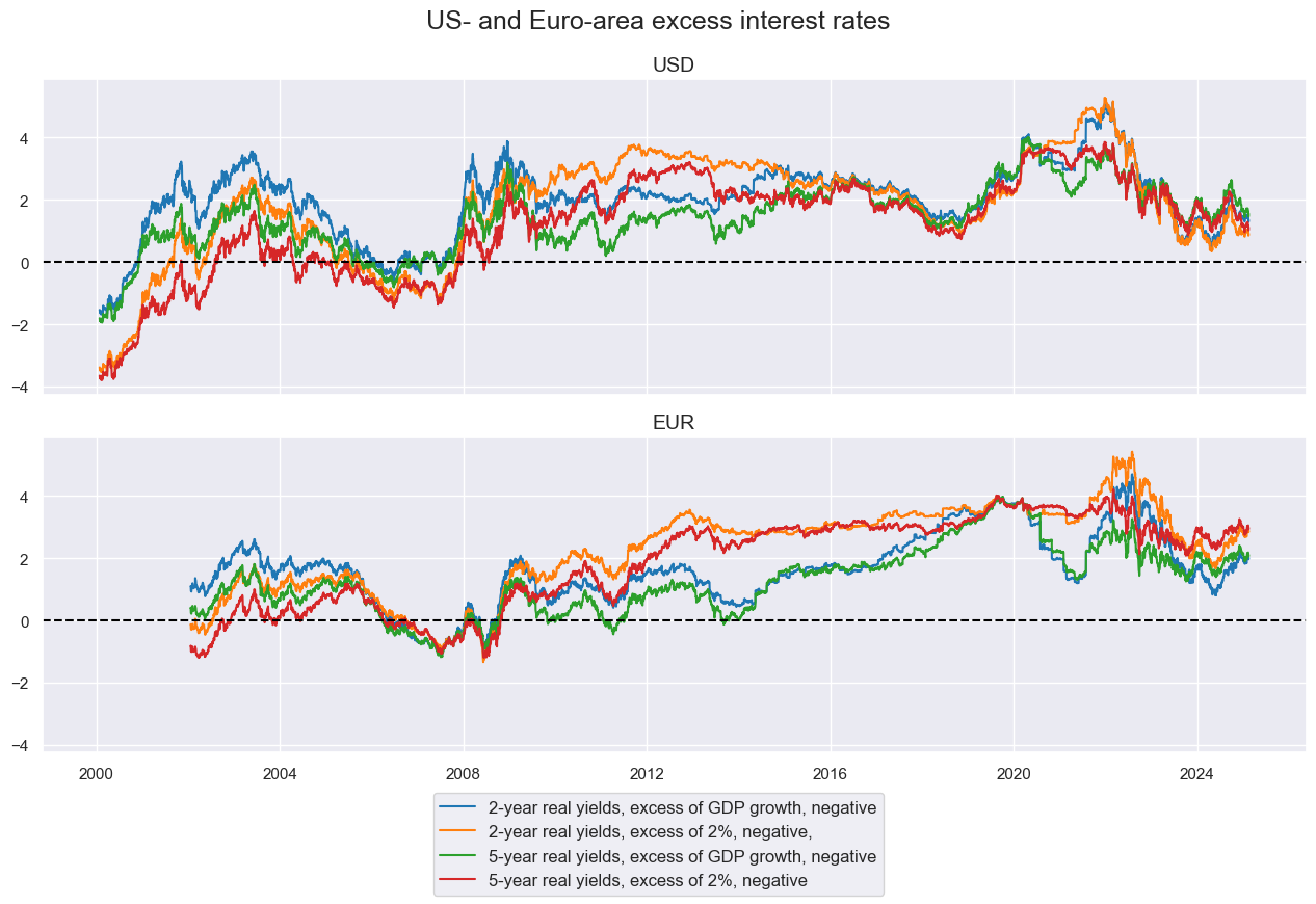
Real interest rate conditions #
# Real rates versus 3-year averages

cidx = cids_cr
calcs = []

for rate in rates:
    calcs.append(f"X{rate}_NEG = - {rate} + RGDP_SA_P1Q1QL4_20QMA")
    calcs.append(f"XX{rate}_NEG = - {rate} + 2")

dfa = msp.panel_calculator(df=dfx, calcs=calcs, cids=cidx)
dfx = msm.update_df(dfx, dfa)

xratns = [f"{x}{rate}_NEG" for rate in rates for x in ["X", "XX"]]
cidx = ["UIG", "EIG"]
xcatx = xratns

msp.view_timelines(
    df=dfx,
    xcats=xcatx,
    cids=cidx,
    title="US- and Euro-area excess interest rates",
    ncol=1,
    same_y=True,
    aspect=3,
    xcat_labels=[
        "2-year real yields, excess of GDP growth, negative",
        "2-year real yields, excess of 2%, negative,",
        "5-year real yields, excess of GDP growth, negative",
        "5-year real yields, excess of 2%, negative",
    ],
    cid_labels=["USD", "EUR"],
)
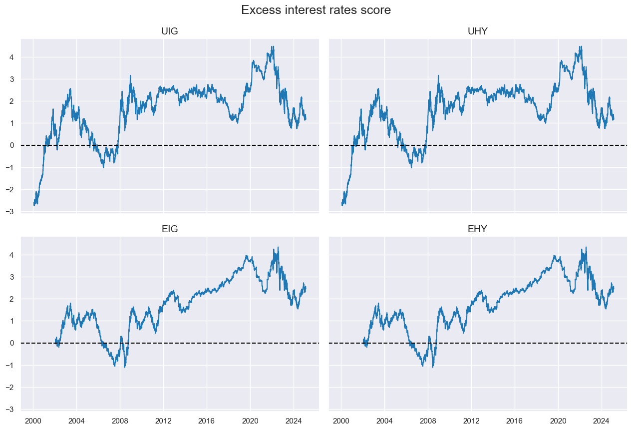
# Composite excess real interest rate measure

xcatx = xratns
cidx = cids_cr

dfa = msp.linear_composite(df=dfx, xcats=xcatx, cids=cidx, new_xcat="XRATES_NEG")
dfx = msm.update_df(dfx, dfa)
cidx = cids_cr
xcatx = ["XRATES_NEG"]

msp.view_timelines(
    df=dfx,
    xcats=xcatx,
    cids=cidx,
    title="Excess interest rates score",
    ncol=2,
    same_y=True,
    aspect=1.5,
)
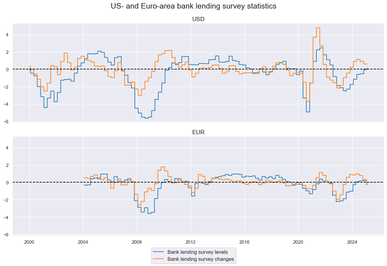
Bank lending surveys #
bls = ["BLSCSCORE_NSA", "BLSCSCORE_NSA_D2Q2QL2"]

cidx = ["UIG", "EIG"]
xcatx = bls

msp.view_timelines(
    df=dfx,
    xcats=xcatx,
    cids=cidx,
    title="US- and Euro-area bank lending survey statistics",
    ncol=1,
    same_y=True,
    aspect=3,
    xcat_labels=["Bank lending survey levels", "Bank lending survey changes"],
    cid_labels=["USD", "EUR"],
)
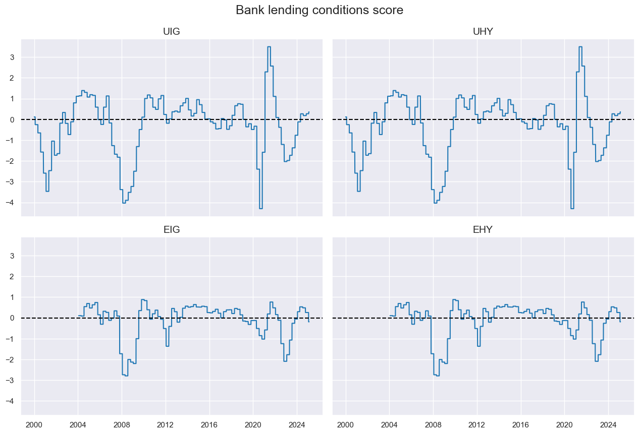
# Composite bank lending supply score
cidx = cids_cr
xcatx = bls

dfa = msp.linear_composite(df=dfx, xcats=xcatx, cids=cids_cr, new_xcat="BLSCOND")
dfx = msm.update_df(dfx, dfa)
cidx = cids_cr
xcatx = ["BLSCOND"]

msp.view_timelines(
    df=dfx,
    xcats=xcatx,
    cids=cidx,
    title="Bank lending conditions score",
    ncol=2,
    same_y=True,
    aspect=1.5,
)
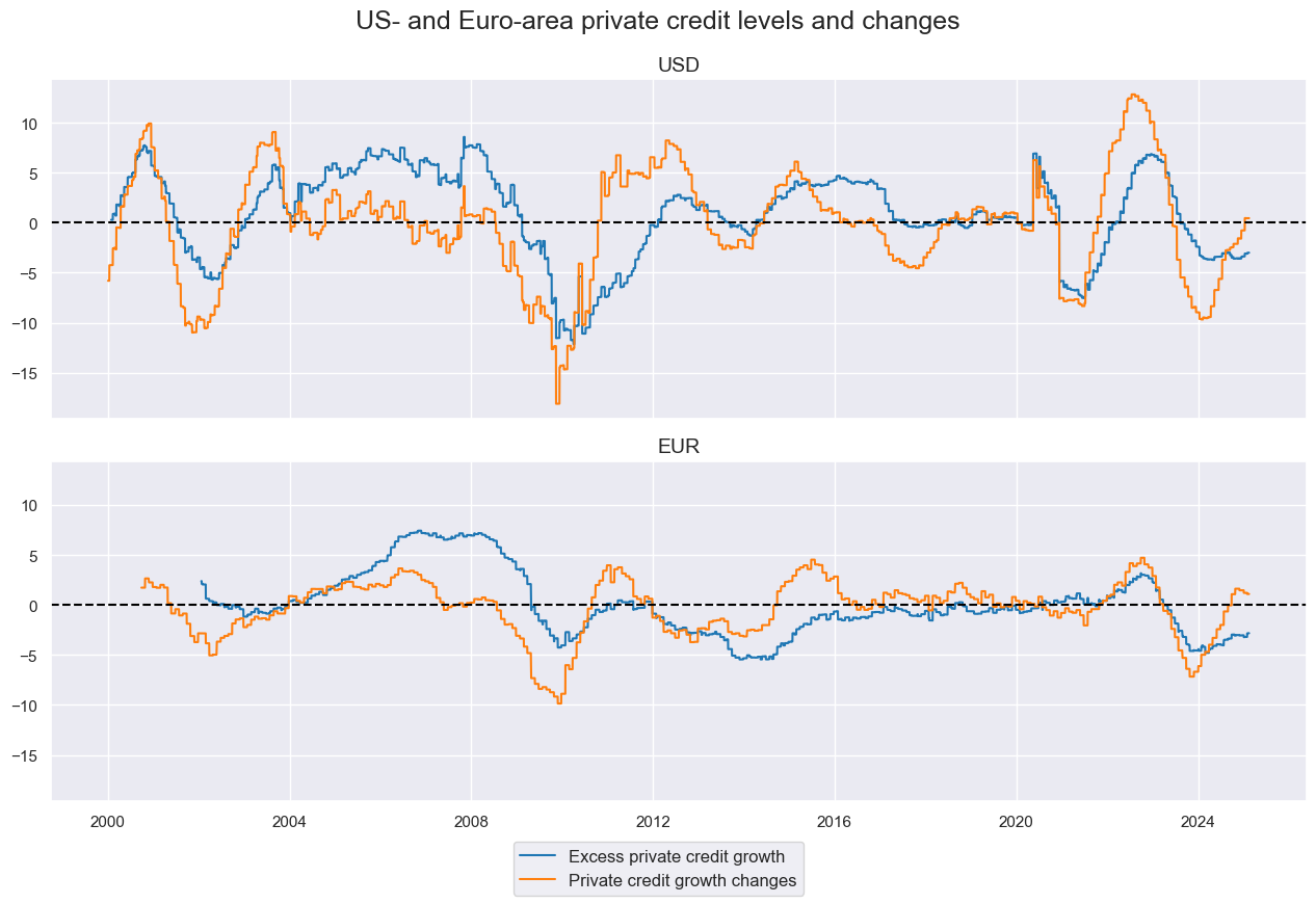
Private credit growth #
# Credit acceleration category

cidx = cids_cr
calcs = []

calcs.append("PCG_DOYA = PCREDITBN_SJA_P1M1ML12_D1M1ML12")
calcs.append("XPCG = PCREDITBN_SJA_P1M1ML12 - INFTEFF_NSA - RGDP_SA_P1Q1QL4_20QMA")

dfa = msp.panel_calculator(df=dfx, calcs=calcs, cids=cidx)
dfx = msm.update_df(dfx, dfa)

xpcgd = ["XPCG", "PCG_DOYA"]
cidx = ["UIG", "EIG"]
xcatx = xpcgd

msp.view_timelines(
    df=dfx,
    xcats=xcatx,
    cids=cidx,
    title="US- and Euro-area private credit levels and changes",
    ncol=1,
    same_y=True,
    aspect=3,
    xcat_labels=["Excess private credit growth", "Private credit growth changes"],
    cid_labels=["USD", "EUR"],
)
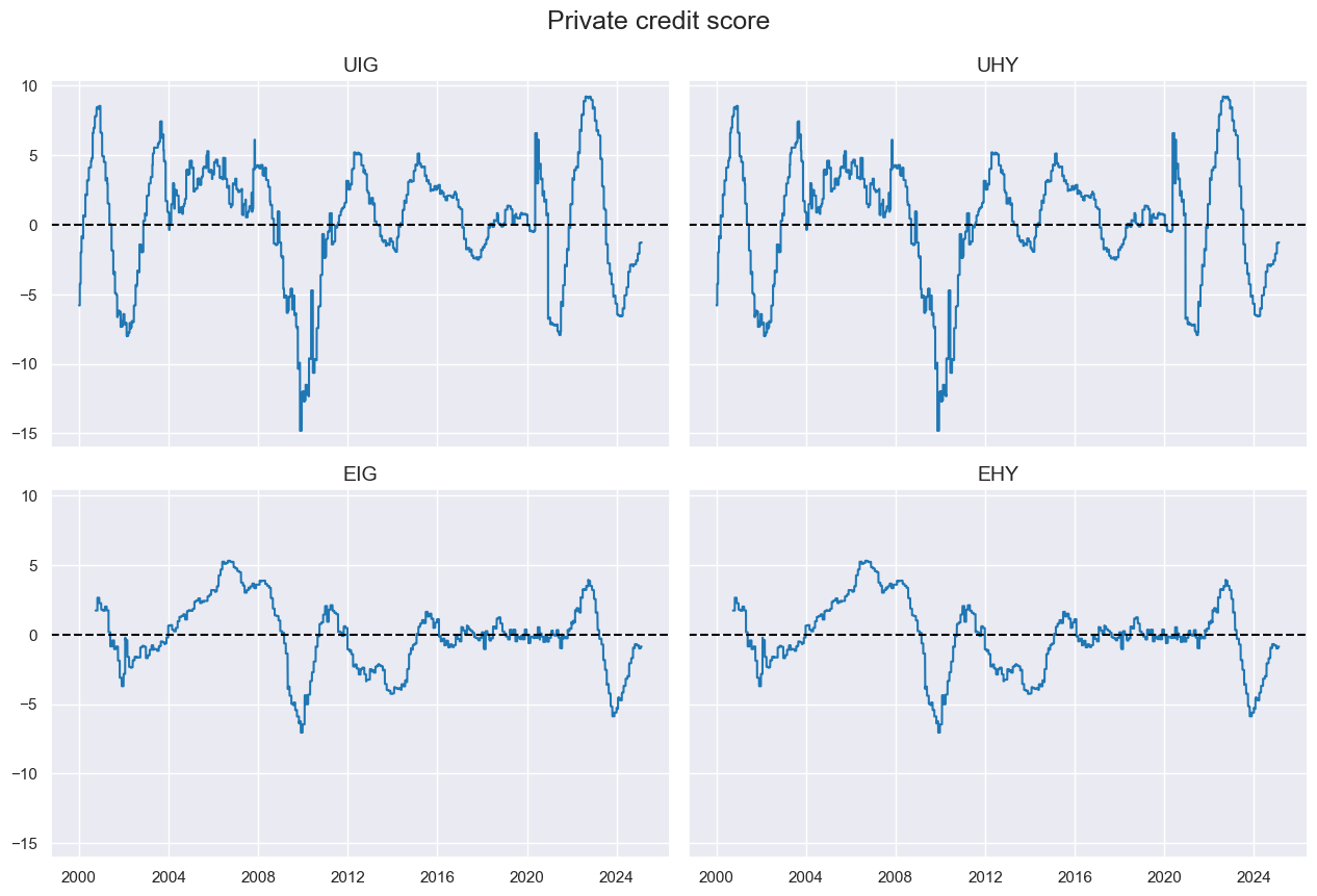
# Single credit expansion category
cidx = cids_cr
xcatx = xpcgd

dfa = msp.linear_composite(df=dfx, xcats=xcatx, cids=cids_cr, new_xcat="XPCREDIT")
dfx = msm.update_df(dfx, dfa)
cidx = cids_cr
xcatx = ["XPCREDIT"]

msp.view_timelines(
    df=dfx,
    xcats=xcatx,
    cids=cidx,
    title="Private credit score",
    ncol=2,
    same_y=True,
    aspect=1.5,
)
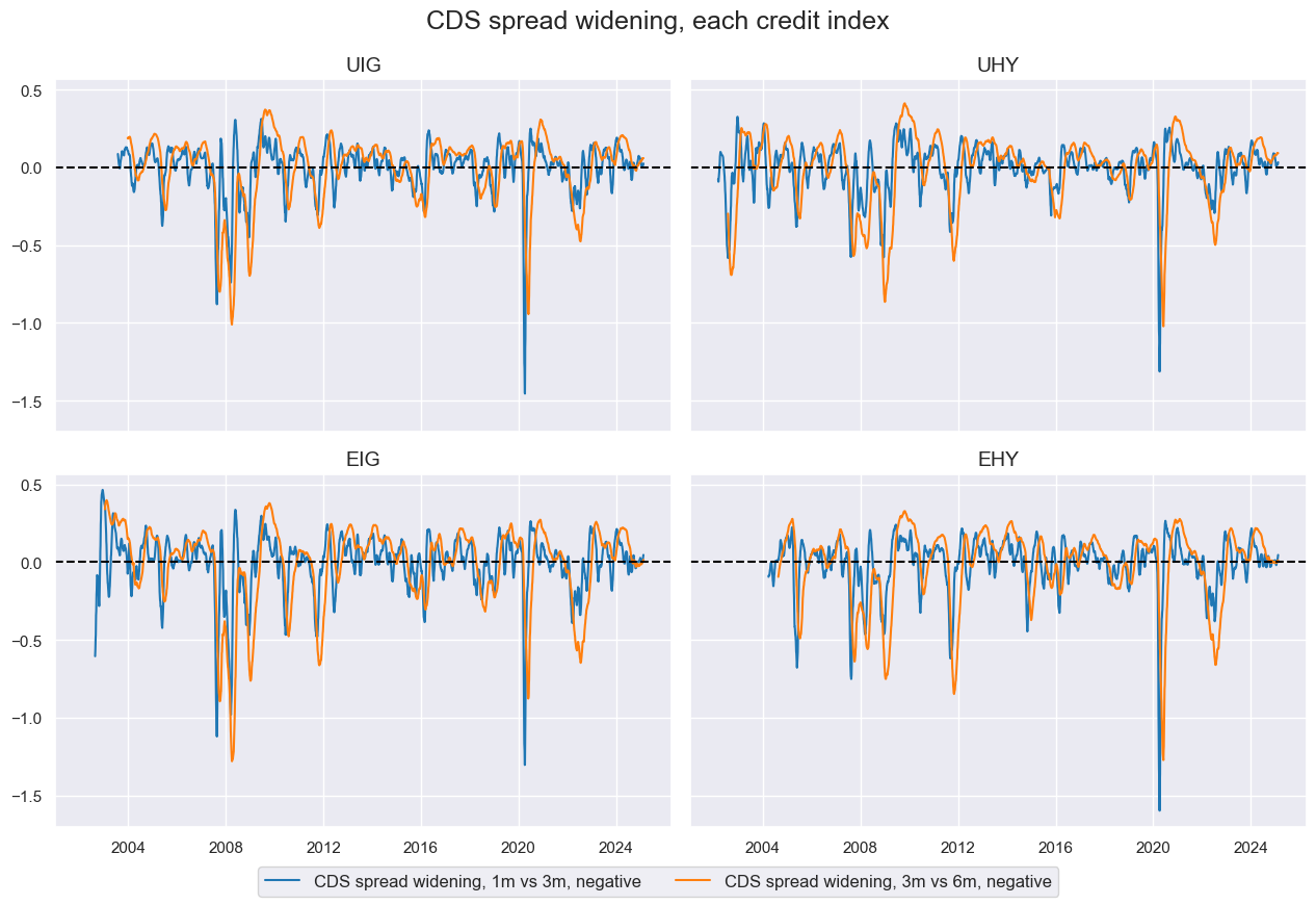
CDS spread widening #
# Credit acceleration category (temp proxy)

cidx = cids_cr
calcs = []

calcs.append("CSPREAD_1MMA = CRCRY_NSA.rolling(21).mean()")
calcs.append("CSPREAD_3MMA = CRCRY_NSA.rolling(21*3).mean()")
calcs.append("CSPREAD_6MMA = CRCRY_NSA.rolling(21*6).mean()")
calcs.append("CSPREAD_3MMA_L1M = CSPREAD_3MMA.shift(21)")
calcs.append("CSPREAD_6MMA_L3M = CSPREAD_6MMA.shift(21*3)")
calcs.append(
    "CSPREAD_P1Mv3M_NEG = - ( CSPREAD_1MMA - CSPREAD_3MMA_L1M ) / CSPREAD_3MMA_L1M"
)
calcs.append(
    "CSPREAD_P3Mv6M_NEG = - ( CSPREAD_3MMA - CSPREAD_6MMA_L3M ) / CSPREAD_6MMA_L3M"
)

dfa = msp.panel_calculator(df=dfx, calcs=calcs, cids=cidx)
dfx = msm.update_df(dfx, dfa)

csp = ["CSPREAD_P1Mv3M_NEG", "CSPREAD_P3Mv6M_NEG"]
cidx = cids_cr
xcatx = csp

msp.view_timelines(
    df=dfx,
    xcats=xcatx,
    cids=cidx,
    title="CDS spread widening, each credit index",
    ncol=2,
    same_y=True,
    aspect=1.5,
    xcat_labels=[
        "CDS spread widening, 1m vs 3m, negative",
        "CDS spread widening, 3m vs 6m, negative",
    ],
)
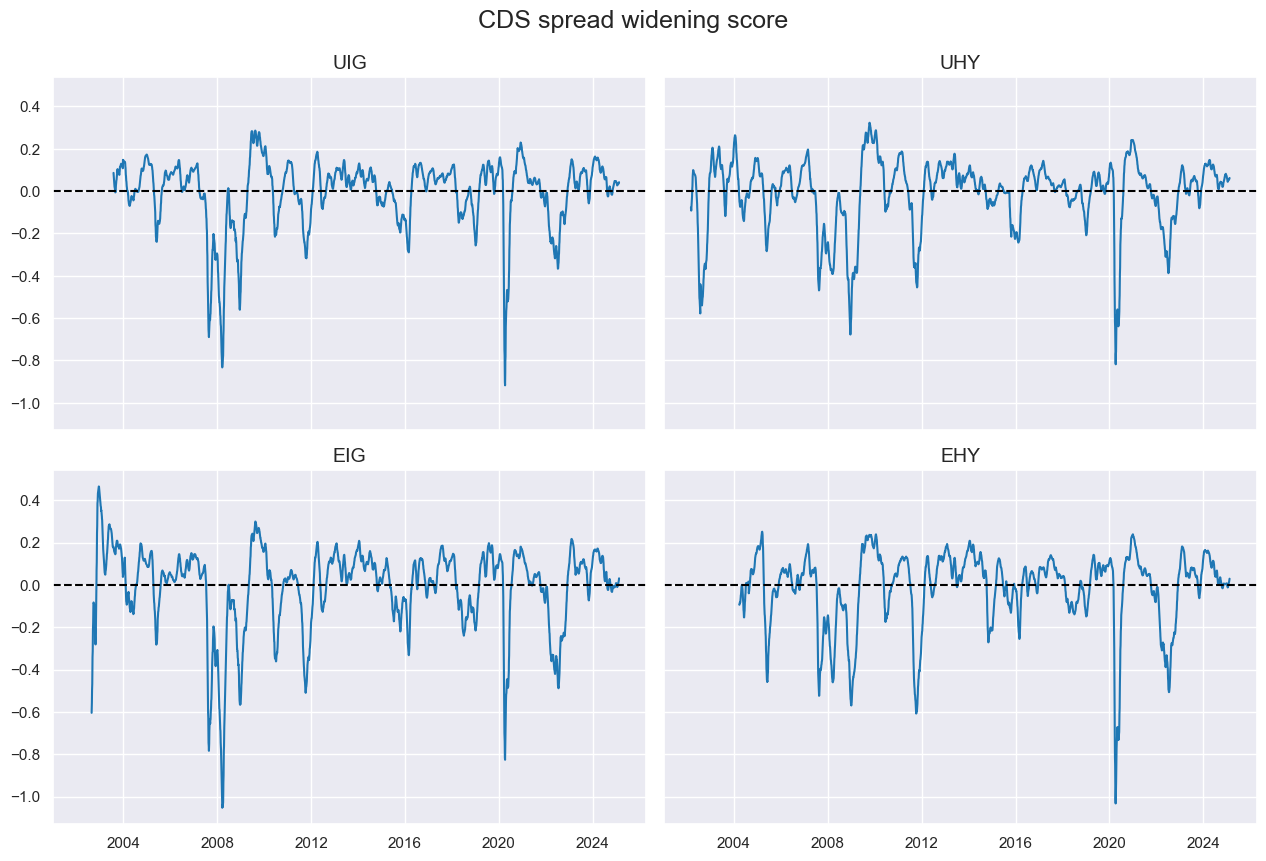
# Single credit expansion category
cidx = cids_cr
xcatx = csp

dfa = msp.linear_composite(
    df=dfx, xcats=xcatx, cids=cids_cr, new_xcat="CSPRWIDE_NEG", start="2002-01-01"
)
dfx = msm.update_df(dfx, dfa)
cidx = cids_cr
xcatx = ["CSPRWIDE_NEG"]

msp.view_timelines(
    df=dfx,
    xcats=xcatx,
    cids=cidx,
    title="CDS spread widening score",
    ncol=2,
    same_y=True,
    aspect=1.5,
)
Transformations and visualizations #
factors = ["BCONFCHG", "XHPI", "XRATES_NEG", "BLSCOND", "XPCREDIT", "CSPRWIDE_NEG"]
Normalization #
# Zn-scores

xcatx = factors
cidx = cids_cr

dfa = pd.DataFrame(columns=list(dfx.columns))

for xc in xcatx:
    dfaa = msp.make_zn_scores(
        dfx,
        xcat=xc,
        cids=cidx,
        sequential=True,
        min_obs=261 * 3,
        neutral="zero",
        pan_weight=0,
        thresh=3,
        postfix="_ZN",
        est_freq="m",
    )
    dfa = msm.update_df(dfa, dfaa)

dfx = msm.update_df(dfx, dfa)

# Modified factor dictionary

factorz = [xcat + "_ZN" for xcat in factors]
Visual checks #
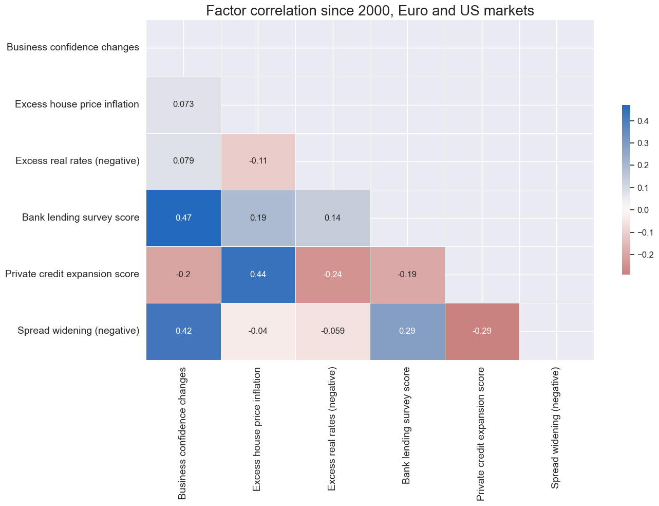
xcatx = factorz
cidx = cids_cr

sdate = "2000-01-01"

renaming_dict = {
    "BCONFCHG_ZN": "Business confidence changes",
    "XHPI_ZN": "Excess house price inflation",
    "XRATES_NEG_ZN": "Excess real rates (negative)",
    "BLSCOND_ZN": "Bank lending survey score",
    "XPCREDIT_ZN": "Private credit expansion score",
    "CSPRWIDE_NEG_ZN": "Spread widening (negative)",
}

msp.correl_matrix(
    dfx,
    xcat_labels=renaming_dict,
    xcats=xcatx,
    cids=cidx,
    start=sdate,
    freq="M",
    title="Factor correlation since 2000, Euro and US markets",
    size=(14, 10),
    annot=True,
)
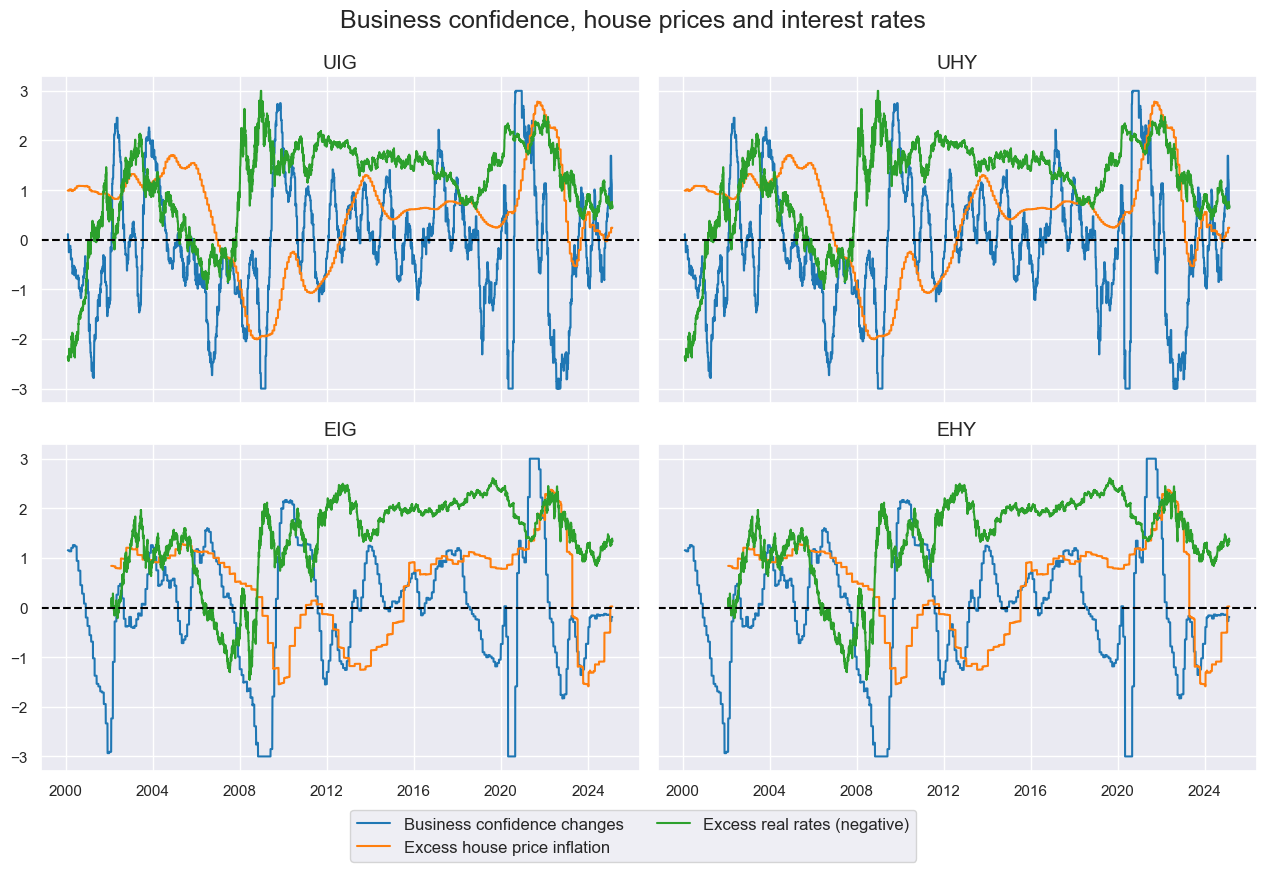
cidx = cids_cr
xcatx = factorz[:3]

msp.view_timelines(
    df=dfx,
    xcats=xcatx,
    cids=cidx,
    title="Business confidence, house prices and interest rates",
    xcat_labels=list(renaming_dict.values())[:3],
    ncol=2,
    same_y=True,
    aspect=1.5,
)
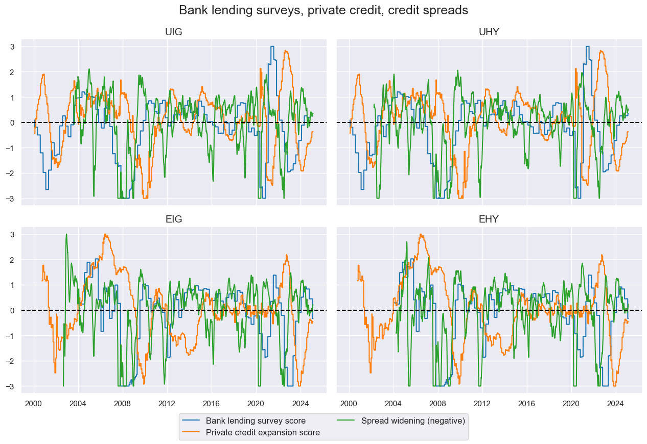
cidx = cids_cr
xcatx = factorz[3:]

msp.view_timelines(
    df=dfx,
    xcats=xcatx,
    cids=cidx,
    title="Bank lending surveys, private credit, credit spreads",
    xcat_labels=list(renaming_dict.values())[3:6],
    ncol=2,
    same_y=True,
    aspect=1.5,
)
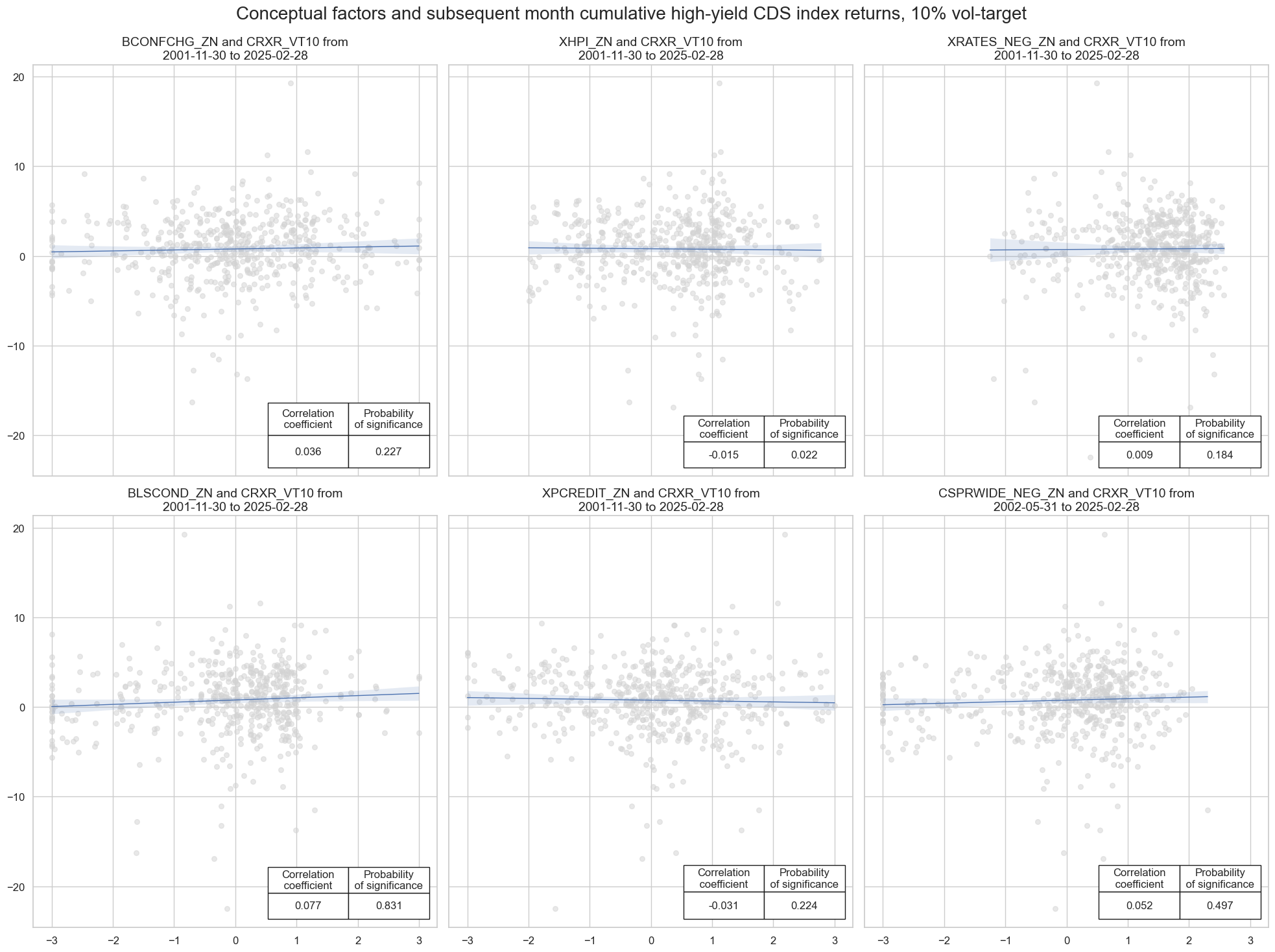
crs = []

for xcat in factorz:
    cr = msp.CategoryRelations(
        df=dfx,
        xcats=[xcat, "CRXR_VT10"],
        cids=cids_hy,
        freq="M",
        lag=1,
        xcat_aggs=["last", "sum"],
        slip=1,
    )
    crs.append(cr)


msv.multiple_reg_scatter(
    cat_rels=crs,
    ncol=3,
    nrow=2,
    coef_box="lower right",
    prob_est="map",
    title="Conceptual factors and subsequent month cumulative high-yield CDS index returns, 10% vol-target",
)
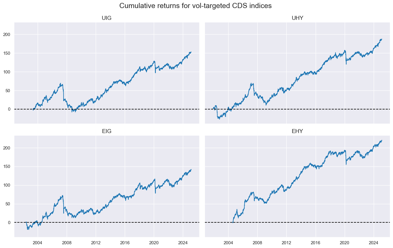
Target return checks #
xcatx = ["CRXR_VT10"]
cidx = cids_cr

msp.view_timelines(
    df=dfx,
    xcats=xcatx,
    cids=cidx,
    cumsum=True,
    title="Cumulative returns for vol-targeted CDS indices ",
    ncol=2,
)
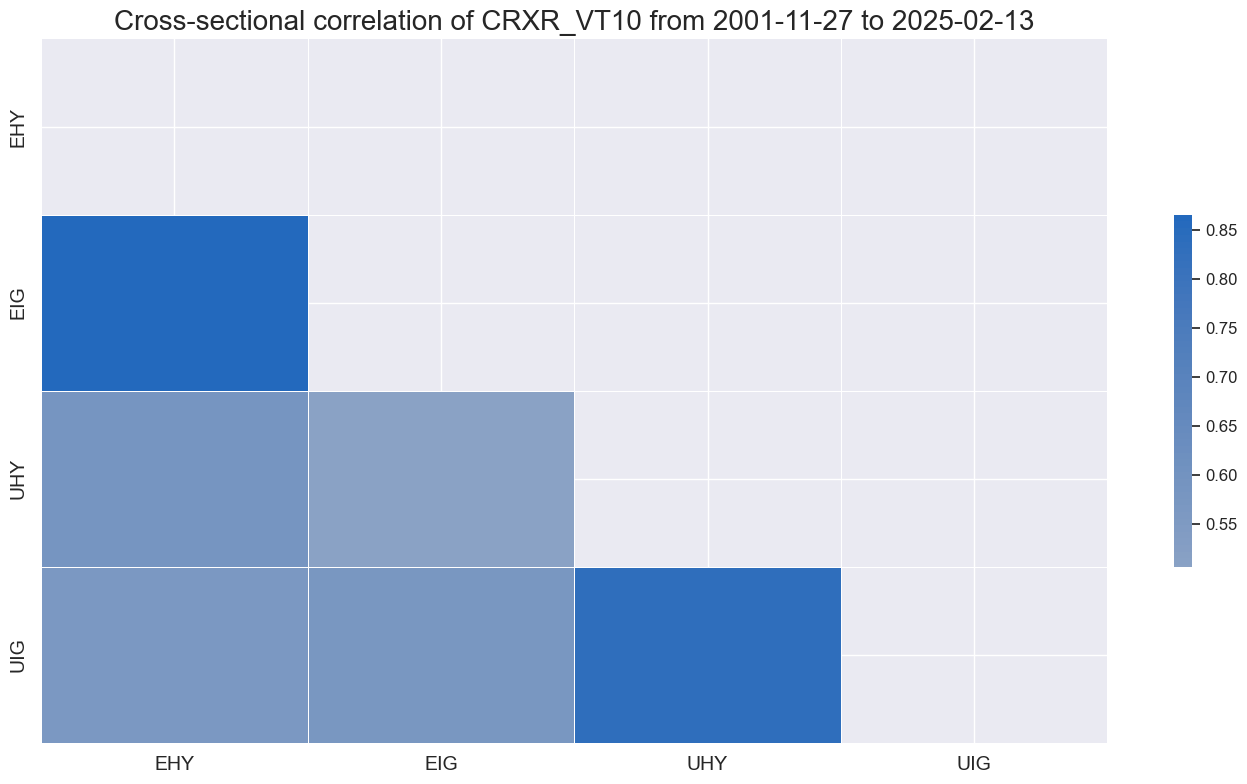
xcatx = ["CRXR_VT10"]
cidx = cids_cr

msp.correl_matrix(df=dfx, xcats=xcatx, cids=cidx, cluster=True)
Preparations for statistical learning #
Convert data to scikit-learn format (redundant) #
cidx = cids_cr
targ = "CRXR_VT10"
xcatx = factorz + [targ]

# Downsample from daily to monthly frequency (features as last and target as sum)
dfw = msm.categories_df(
    df=dfx,
    xcats=xcatx,
    cids=cidx,
    freq="M",
    lag=1,
    xcat_aggs=["last", "sum"],
)

# Drop rows with missing values and assign features and target
dfw.dropna(inplace=True)
X_cr = dfw.iloc[:, :-1]
y_cr = dfw.iloc[:, -1]
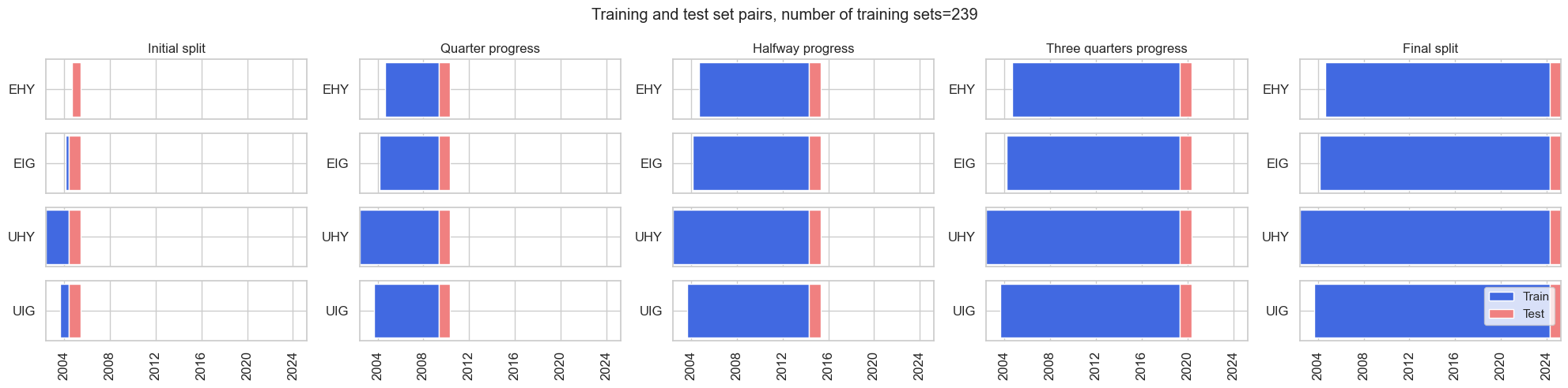
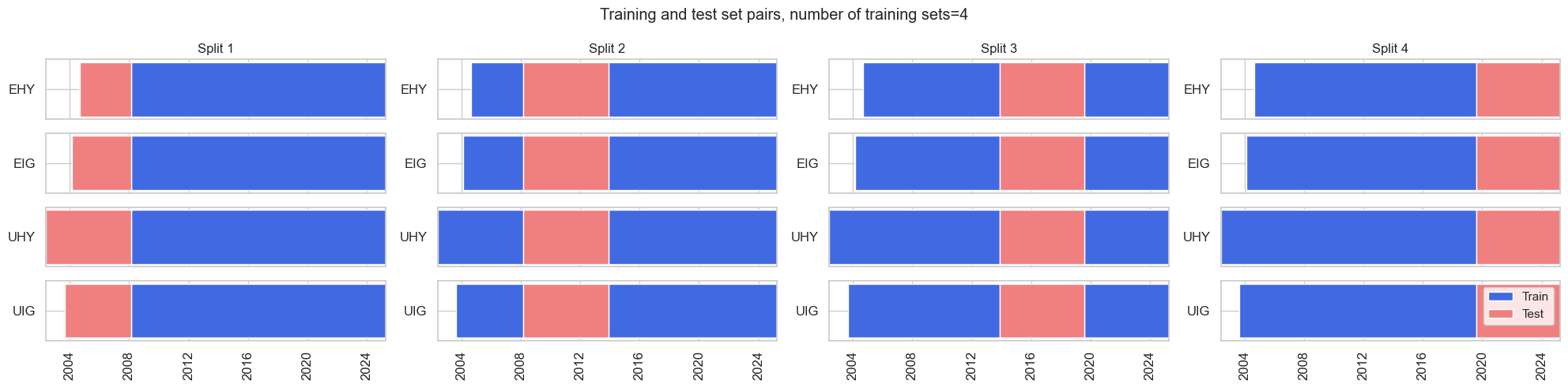
Define cross-validation dynamics #
Visualize back test dynamics (with a one year forward window for visualization purposes).
-
The first set comprises the first 2 years of the panel.
-
A one month forward forecast is made.
Noting longer training times for random forests, that particular model is retrained every quarter.
# Initial split dynamics
min_cids = 1
min_periods = 12 * 2
test_size = 1

# Visualize back test pipeline
msl.ExpandingIncrementPanelSplit(
    train_intervals=test_size,
    test_size=12,
    min_cids=min_cids,
    min_periods=min_periods,
).visualise_splits(X_cr, y_cr)
# Cross-validation dynamics
splitters = {
    "Expanding": msl.ExpandingKFoldPanelSplit(4),
    "Rolling": msl.RollingKFoldPanelSplit(4),
}

split_functions = None
scorers = {"BAC": make_scorer(balanced_accuracy_score)}
cv_summary = "median"
splitters["Expanding"].visualise_splits(X_cr, y_cr)
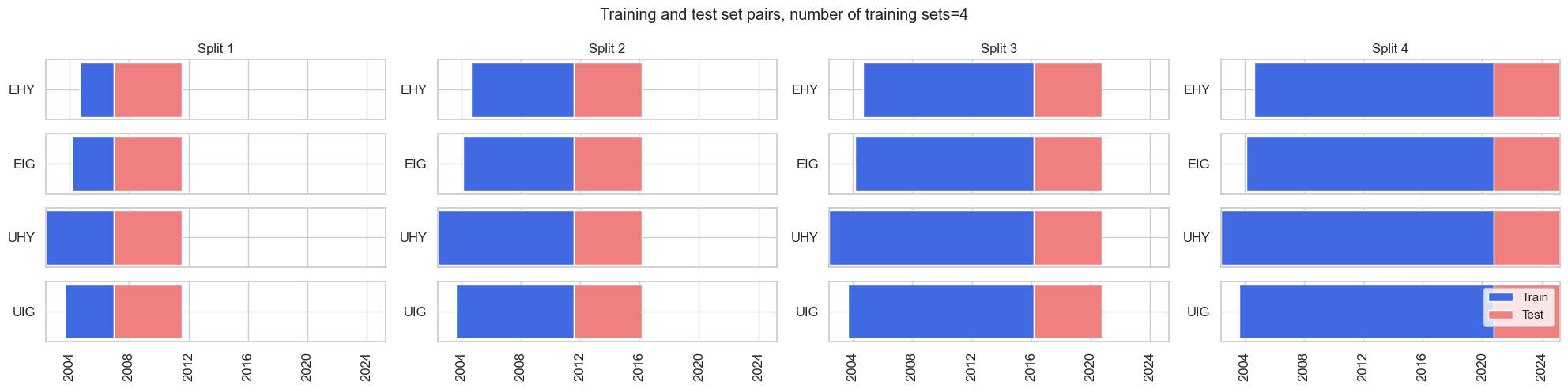
splitters["Rolling"].visualise_splits(X_cr, y_cr)
Signal generation #
Pooled panel models #
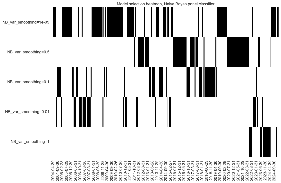
Naive Bayes #
so_nb = msl.SignalOptimizer(
df=dfx,
xcats=factorz + ["CRXR_VT10"],
cids=cids_cr,
freq="M",
lag=1,
xcat_aggs=["last", "sum"],
generate_labels=lambda x: 1 if x >= 0 else -1,
)
so_nb.calculate_predictions(
name="NB",
models={"NB": GaussianNB()},
hyperparameters={
"NB": {
"var_smoothing": [1e-9, 1e-2, 1e-1, 5e-1, 1],
},
},
scorers=scorers,
inner_splitters=splitters,
min_cids=min_cids,
min_periods=min_periods,
test_size=test_size,
n_jobs_outer=-1,
cv_summary=cv_summary,
split_functions=split_functions,
)
so_nb.models_heatmap(
"NB", title="Model selection heatmap, Naive Bayes panel classifier"
)
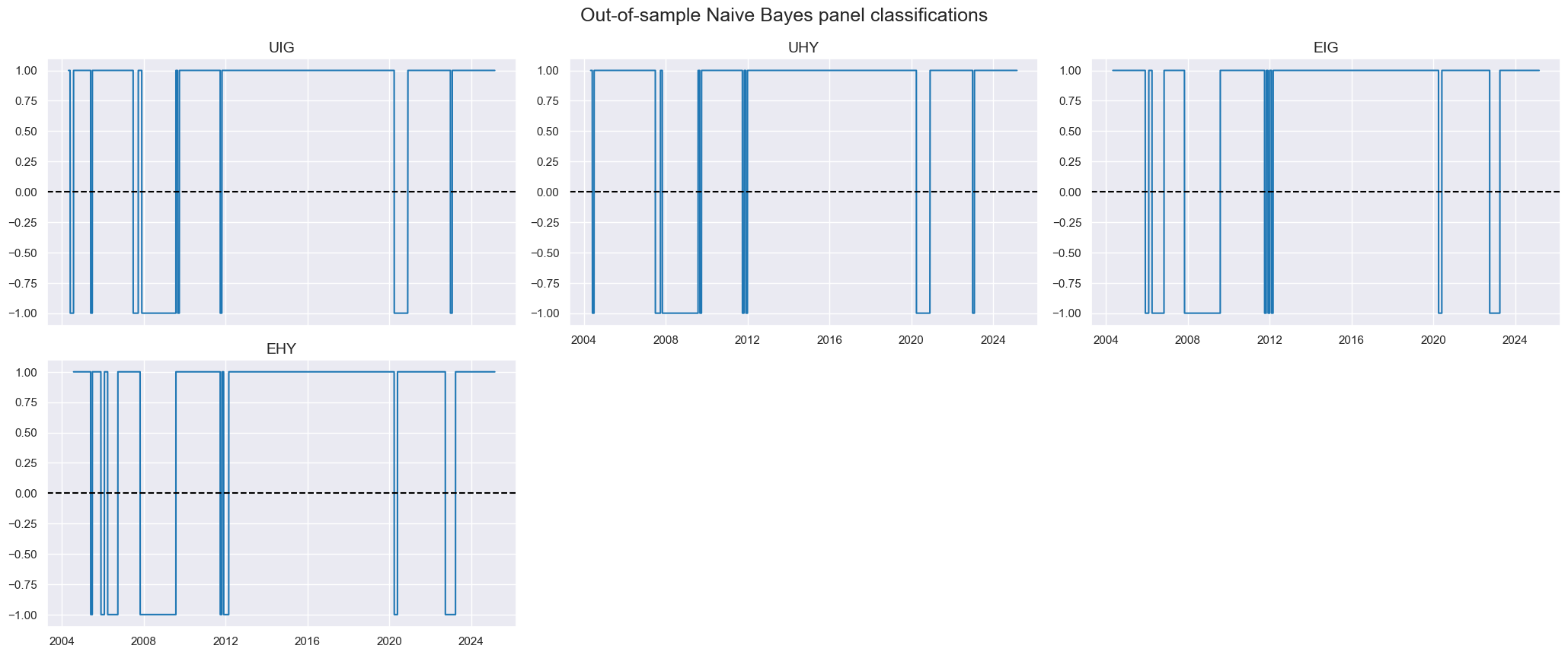
dfa = so_nb.get_optimized_signals("NB")
dfx = msm.update_df(dfx, dfa)
msp.view_timelines(
    df=dfx,
    xcats=["NB"],
    cids=cids_cr,
    title="Out-of-sample Naive Bayes panel classifications",
    same_y=False,
)
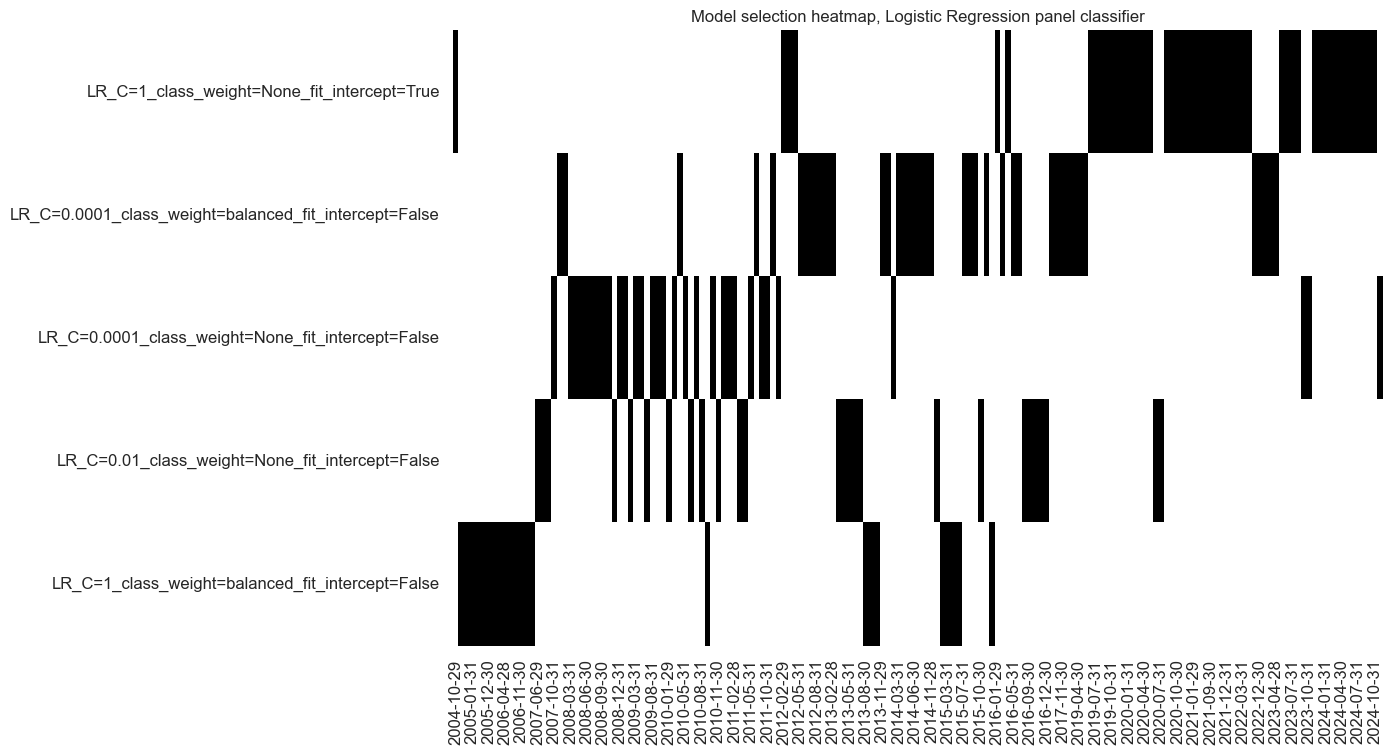
Logistic regression #
so_lr = msl.SignalOptimizer(
    df=dfx,
    xcats=factorz + ["CRXR_VT10"],
    cids=cids_cr,
    freq="M",
    lag=1,
    xcat_aggs=["last", "sum"],
    generate_labels=lambda x: 1 if x >= 0 else -1,
)

so_lr.calculate_predictions(
    name="LR",
    models={
        "LR": LogisticRegression(random_state=42),
    },
    hyperparameters={
        "LR": {
            "class_weight": ["balanced", None],
            "C": [1, 1e-2, 1e-4, 1e-6, 1e-8],
            "fit_intercept": [True, False],
        },
    },
    scorers=scorers,
    inner_splitters=splitters,
    min_cids=min_cids,
    min_periods=min_periods,
    cv_summary=cv_summary,
    test_size=test_size,
    n_jobs_outer=-1,
    split_functions=split_functions,
)

so_lr.models_heatmap(
    "LR", title="Model selection heatmap, Logistic Regression panel classifier"
)

dfa = so_lr.get_optimized_signals("LR")
dfx = msm.update_df(dfx, dfa)
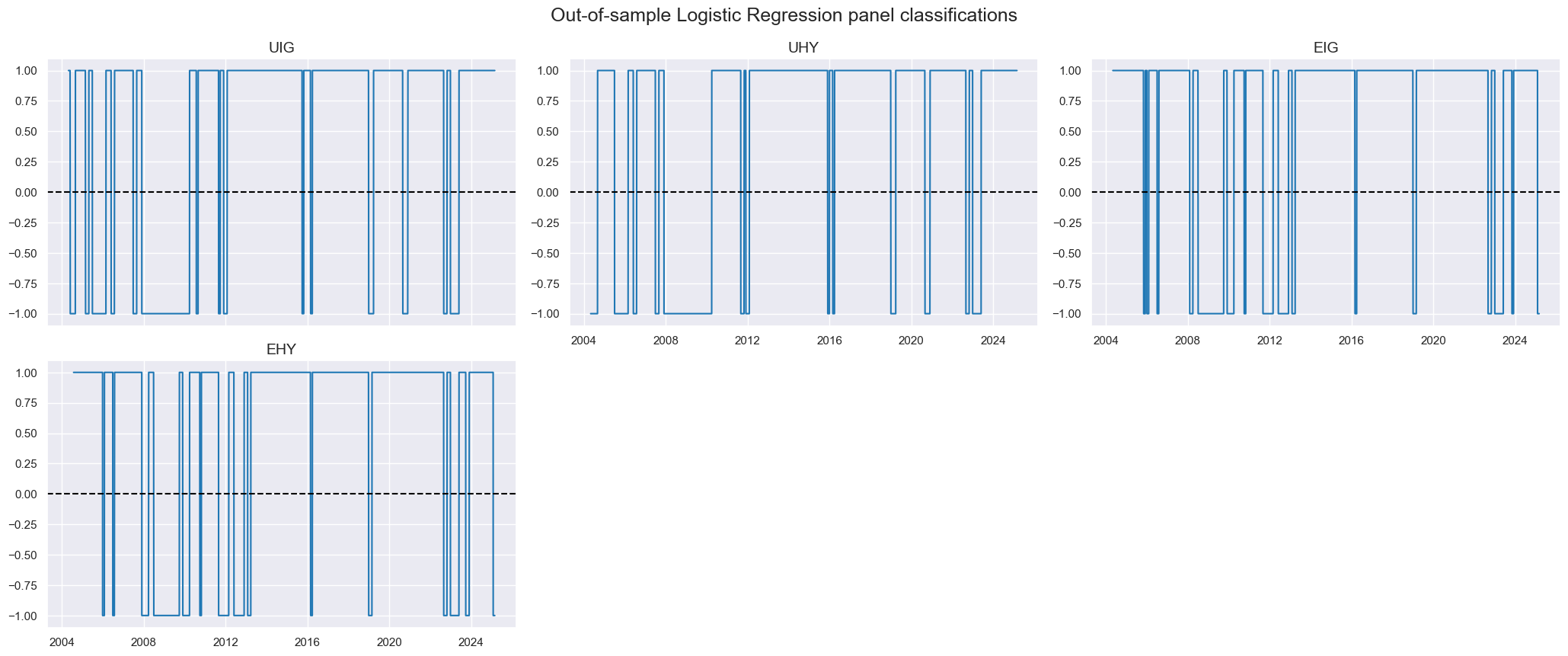
msp.view_timelines(
    df=dfx,
    xcats=["LR"],
    cids=cids_cr,
    title="Out-of-sample Logistic Regression panel classifications",
    same_y=False,
)
K Nearest Neighbors #
so_knn = msl.SignalOptimizer(
df=dfx,
xcats=factorz + ["CRXR_VT10"],
cids=cids_cr,
freq="M",
lag=1,
xcat_aggs=["last", "sum"],
generate_labels=lambda x: 1 if x >= 0 else -1,
)
so_knn.calculate_predictions(
name="KNN",
models={
"KNN": msl.KNNClassifier(),
},
hyperparameters={
"KNN": {
"n_neighbors": ["sqrt", 0.1, 0.25],
"weights": ["uniform", "distance"],
},
},
scorers=scorers,
inner_splitters=splitters,
min_cids=min_cids,
min_periods=min_periods, # 2 years
test_size=test_size,
n_jobs_outer=-1,
cv_summary=cv_summary,
)
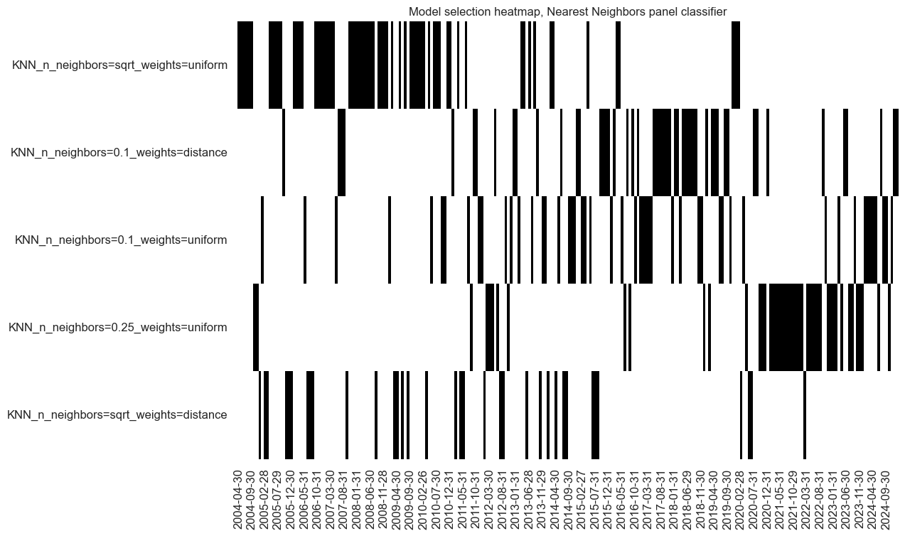
so_knn.models_heatmap(
"KNN", title="Model selection heatmap, Nearest Neighbors panel classifier"
)
dfa = so_knn.get_optimized_signals("KNN")
dfx = msm.update_df(dfx, dfa)
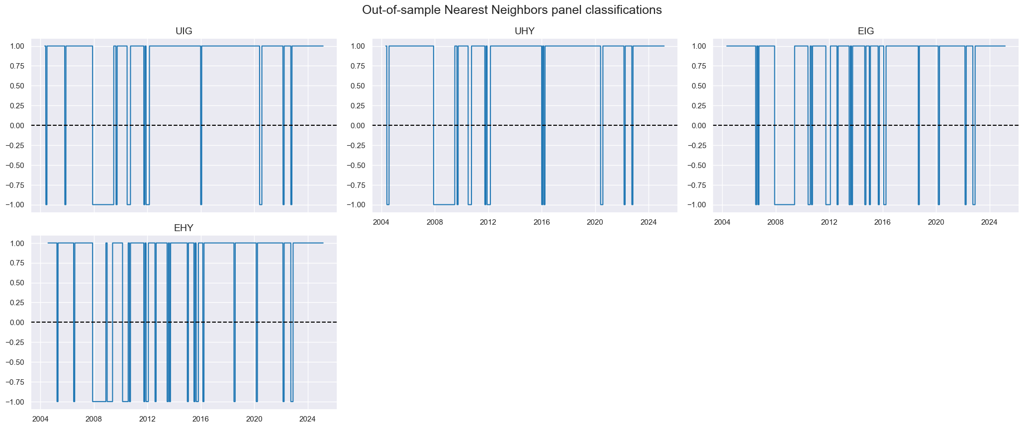
msp.view_timelines(
    df=dfx,
    title="Out-of-sample Nearest Neighbors panel classifications",
    xcats=["KNN"],
    cids=cids_cr,
    same_y=False,
)
Random forest #
so_rf = msl.SignalOptimizer(
df=dfx,
xcats=factorz + ["CRXR_VT10"],
cids=cids_cr,
freq="M",
lag=1,
xcat_aggs=["last", "sum"],
generate_labels=lambda x: 1 if x >= 0 else -1,
)
so_rf.calculate_predictions(
name="RF",
models={
"RF": RandomForestClassifier(
random_state=42,
n_estimators=500,
),
},
hyperparameters={
"RF": {
"class_weight": [None, "balanced"],
"max_features": ["sqrt", None],
"max_samples": [0.25, 0.1],
"min_samples_leaf": [1, 5],
},
},
scorers=scorers,
inner_splitters=splitters,
cv_summary=cv_summary,
min_cids=min_cids,
min_periods=min_periods, # 2 years
test_size=3,
split_functions=split_functions,
n_jobs_outer=-1,
)
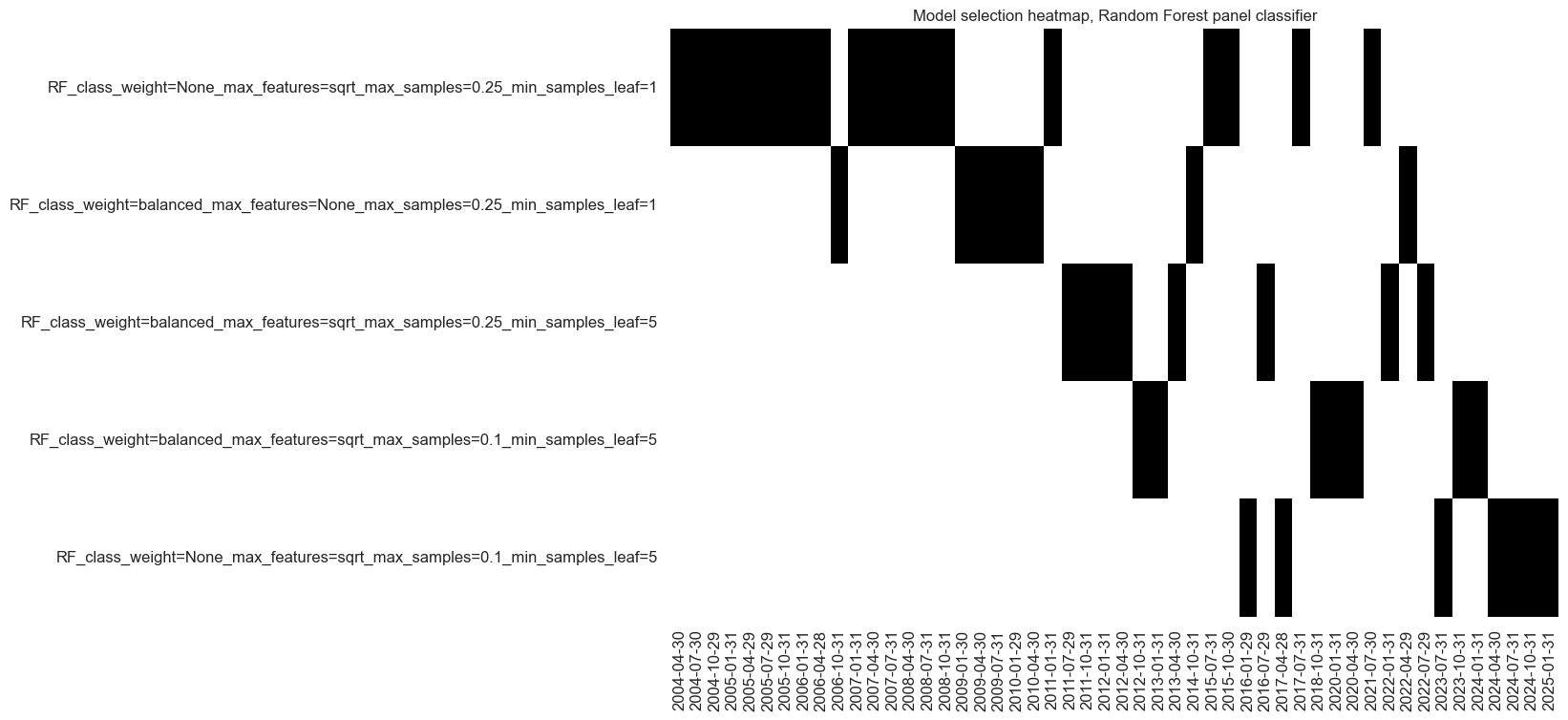
so_rf.models_heatmap(
"RF", title="Model selection heatmap, Random Forest panel classifier"
)
dfa = so_rf.get_optimized_signals("RF")
dfx = msm.update_df(dfx, dfa)
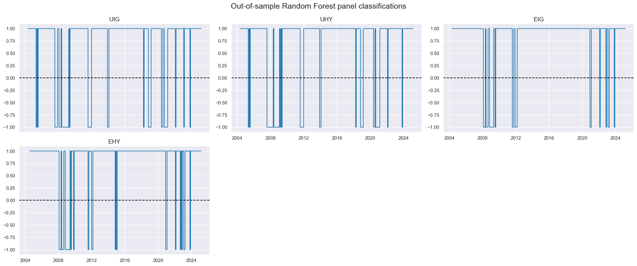
msp.view_timelines(
    df=dfx,
    title="Out-of-sample Random Forest panel classifications",
    xcats=["RF"],
    cids=cids_cr,
    same_y=False,
)
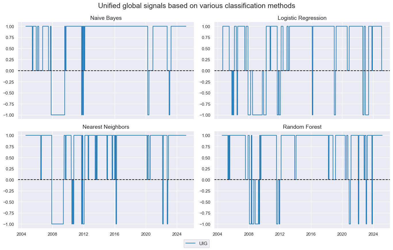
Global signal #
For each of the signals previously calculated, we use majority voting to determine a single global signal that is applied to all cross-sections.
mods = ["NB", "LR", "KNN", "RF"]

for mod in mods:
    dfa = msp.panel_calculator(
        df=dfx,
        calcs=[f"{mod}_GLB = iEIG_{mod} + iEHY_{mod} + iUIG_{mod} + iUHY_{mod}"],
        cids=cids_cr,
    ).dropna()
    dfa["value"] = dfa["value"].apply(lambda x: 1 if x > 0 else -1 if x < 0 else 0)
    dfx = msm.update_df(dfx, dfa)

cidx = ["UIG"]
xcatx = [mod + "_GLB" for mod in mods]
msp.view_timelines(
    df=dfx,
    cids=cidx,
    xcats=xcatx,
    same_y=False,
    ncol=2,
    xcat_grid=True,
    title="Unified global signals based on various classification methods",
    xcat_labels=["Naive Bayes", "Logistic Regression", "Nearest Neighbors", "Random Forest"]
)
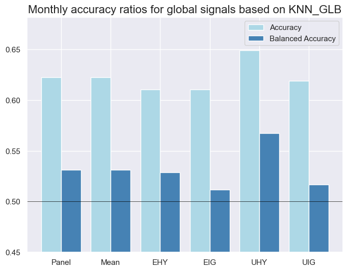
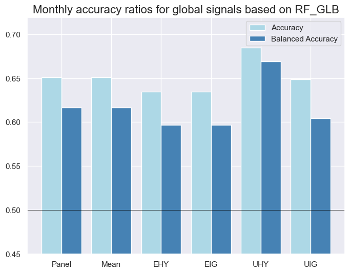
Signal value checks #
Global signal #
Accuracy check #
## Compare optimized signals with simple average z-scores

srr = mss.SignalReturnRelations(
    df=dfx,
    rets=["CRXR_VT10"],
    sigs=["NB_GLB", "LR_GLB", "KNN_GLB", "RF_GLB"],
    cids=cids_cr,
    cosp=True,
    freqs=["M"],
    agg_sigs=["last"],
    start="2002-12-31",
    slip=1,
)

selcols = [
    "accuracy",
    "bal_accuracy",
    "pos_sigr",  # In the regime classification setting, this is less relevant
    "pos_retr",
]

srr.multiple_relations_table().round(3)  # [selcols]
| accuracy | bal_accuracy | pos_sigr | pos_retr | pos_prec | neg_prec | pearson | pearson_pval | kendall | kendall_pval | auc | ||||
|---|---|---|---|---|---|---|---|---|---|---|---|---|---|---|
| Return | Signal | Frequency | Aggregation | |||||||||||
| CRXR_VT10 | KNN_GLB | M | last | 0.622 | 0.531 | 0.887 | 0.642 | 0.649 | 0.413 | 0.020 | 0.532 | 0.015 | 0.561 | 0.514 |
| LR_GLB | M | last | 0.576 | 0.493 | 0.814 | 0.627 | 0.624 | 0.362 | -0.025 | 0.427 | -0.036 | 0.149 | 0.496 | |
| NB_GLB | M | last | 0.627 | 0.555 | 0.883 | 0.636 | 0.649 | 0.462 | 0.064 | 0.043 | 0.035 | 0.166 | 0.525 | |
| RF_GLB | M | last | 0.651 | 0.617 | 0.909 | 0.637 | 0.658 | 0.575 | 0.085 | 0.007 | 0.055 | 0.031 | 0.542 |
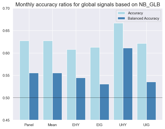
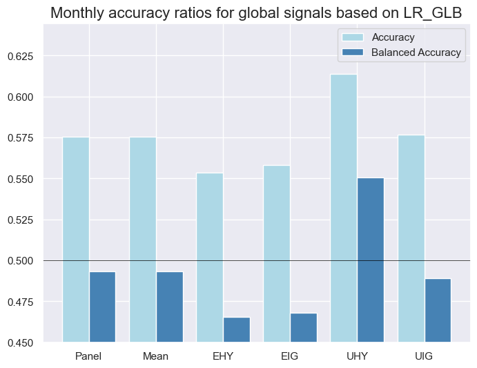
xcatx = ["NB_GLB", "LR_GLB", "KNN_GLB", "RF_GLB"]
for xcat in xcatx:
    srr.accuracy_bars(
        ret="CRXR_VT10",
        sigs=xcat,
        title=f"Monthly accuracy ratios for global signals based on {xcat}",
    )
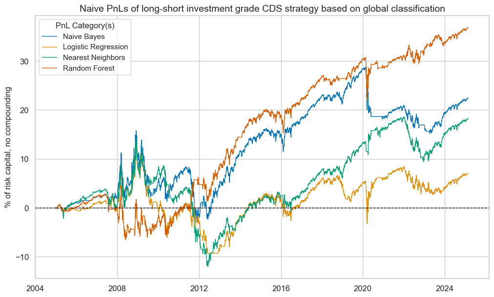
Naive PnL #
Simple notional positions #
sigx = ["NB_GLB", "LR_GLB", "KNN_GLB", "RF_GLB"]
cidx = cids_ig

pnls = msn.NaivePnL(
    df=dfx,
    ret="CRXR_NSA",
    sigs=sigx,
    cids=cidx,
    start="2004-12-31",
    bms=["USD_GB10YXR_NSA", "USD_EQXR_NSA"],
)
for sig in sigx:
    pnls.make_pnl(
        sig=sig,
        sig_op="raw",
        sig_add=0,
        sig_mult=1,
        rebal_freq="monthly",
        rebal_slip=1,
        # vol_scale=10,
    )

pnls.plot_pnls(
    title="Naive PnLs of long-short investment grade CDS strategy based on global classification",
    xcat_labels=[
        "Naive Bayes",
        "Logistic Regression",
        "Nearest Neighbors",
        "Random Forest",
    ],
    title_fontsize=14,
)
pnls.evaluate_pnls(pnl_cats=["PNL_" + sig for sig in sigx])
| xcat | PNL_NB_GLB | PNL_LR_GLB | PNL_KNN_GLB | PNL_RF_GLB |
|---|---|---|---|---|
| Return % | 1.1135 | 0.34396 | 0.90514 | 1.828387 |
| St. Dev. % | 3.923994 | 3.811226 | 3.74399 | 3.604658 |
| Sharpe Ratio | 0.283767 | 0.090249 | 0.241758 | 0.507229 |
| Sortino Ratio | 0.394816 | 0.12678 | 0.341422 | 0.72707 |
| Max 21-Day Draw % | -8.675489 | -8.675489 | -6.362013 | -8.675489 |
| Max 6-Month Draw % | -11.285529 | -10.279486 | -11.152464 | -8.985967 |
| Peak to Trough Draw % | -18.698017 | -22.894696 | -25.831003 | -11.118991 |
| Top 5% Monthly PnL Share | 1.422803 | 4.468367 | 1.781921 | 0.840486 |
| USD_GB10YXR_NSA correl | -0.040796 | 0.010483 | -0.040389 | -0.088499 |
| USD_EQXR_NSA correl | 0.137493 | 0.095487 | 0.110031 | 0.236717 |
| Traded Months | 243 | 243 | 243 | 243 |
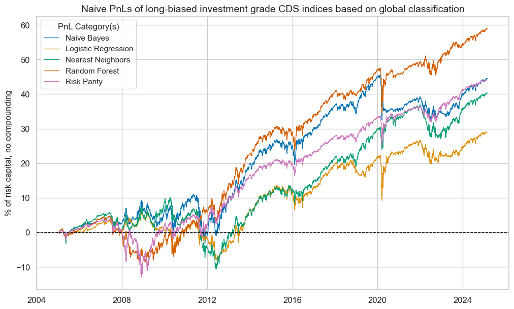
sigx = ["NB_GLB", "LR_GLB", "KNN_GLB", "RF_GLB"]
cidx = cids_ig

pnls = msn.NaivePnL(
    df=dfx,
    ret="CRXR_NSA",
    sigs=sigx,
    cids=cidx,
    start="2004-12-31",
    bms=["USD_GB10YXR_NSA", "USD_EQXR_NSA"],
)
for sig in sigx:
    pnls.make_pnl(
        sig=sig,
        sig_op="raw",
        sig_add=0.5,
        sig_mult=1,
        rebal_freq="monthly",
        neutral="zero",
        rebal_slip=1,
        # vol_scale=10,
    )

pnls.make_long_pnl(vol_scale=None, label="Long only")

pnls.plot_pnls(
    title="Naive PnLs of long-biased investment grade CDS indices based on global classification",
    xcat_labels=[
        "Naive Bayes",
        "Logistic Regression",
        "Nearest Neighbors",
        "Random Forest",
        "Risk Parity",
    ],
    title_fontsize=14,
)
pnls.evaluate_pnls(pnl_cats=["PNL_" + sig for sig in sigx] + ["Long only"])
| xcat | PNL_NB_GLB | PNL_LR_GLB | PNL_KNN_GLB | PNL_RF_GLB | Long only |
|---|---|---|---|---|---|
| Return % | 2.210535 | 1.440864 | 2.002175 | 2.925422 | 2.197246 |
| St. Dev. % | 4.613926 | 4.375357 | 4.38808 | 4.626966 | 4.062352 |
| Sharpe Ratio | 0.479101 | 0.329313 | 0.456276 | 0.632255 | 0.54088 |
| Sortino Ratio | 0.671469 | 0.463916 | 0.653023 | 0.904603 | 0.772765 |
| Max 21-Day Draw % | -13.013234 | -13.013234 | -6.403795 | -13.013234 | -8.675489 |
| Max 6-Month Draw % | -13.878189 | -10.181213 | -13.878189 | -10.181212 | -11.587299 |
| Peak to Trough Draw % | -14.194191 | -15.090157 | -20.853717 | -13.804806 | -16.774382 |
| Top 5% Monthly PnL Share | 0.84618 | 1.168736 | 0.920672 | 0.635319 | 0.750353 |
| USD_GB10YXR_NSA correl | -0.159647 | -0.122637 | -0.165843 | -0.193545 | -0.284131 |
| USD_EQXR_NSA correl | 0.40958 | 0.391762 | 0.40159 | 0.476238 | 0.66547 |
| Traded Months | 243 | 243 | 243 | 243 | 243 |
sigx = ["NB_GLB", "LR_GLB", "KNN_GLB", "RF_GLB"]
cidx = cids_hy
pnls = msn.NaivePnL(
df=dfx,
ret="CRXR_NSA",
sigs=sigx,
cids=cidx,
start="2004-12-31",
bms=["USD_GB10YXR_NSA", "USD_EQXR_NSA"],
)
for sig in sigx:
pnls.make_pnl(
sig=sig,
sig_op="raw",
sig_add=0,
sig_mult=1,
rebal_freq="monthly",
rebal_slip=1,
# vol_scale=10,
)
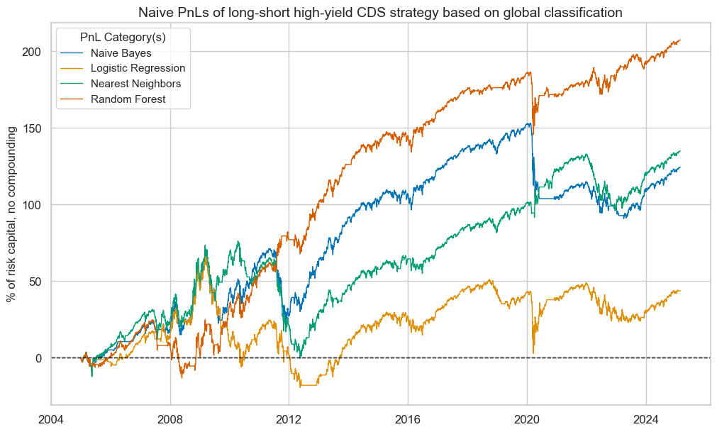
pnls.plot_pnls(
title="Naive PnLs of long-short high-yield CDS strategy based on global classification",
xcat_labels=[
"Naive Bayes",
"Logistic Regression",
"Nearest Neighbors",
"Random Forest",
],
title_fontsize=14,
)
pnls.evaluate_pnls(pnl_cats=["PNL_" + sig for sig in sigx])
| xcat | PNL_NB_GLB | PNL_LR_GLB | PNL_KNN_GLB | PNL_RF_GLB |
|---|---|---|---|---|
| Return % | 6.16179 | 2.167904 | 6.687169 | 10.28211 |
| St. Dev. % | 14.211154 | 14.073087 | 13.542657 | 13.495598 |
| Sharpe Ratio | 0.433588 | 0.154046 | 0.493786 | 0.761886 |
| Sortino Ratio | 0.601779 | 0.215091 | 0.704502 | 1.108458 |
| Max 21-Day Draw % | -39.639918 | -39.639918 | -26.586614 | -39.639918 |
| Max 6-Month Draw % | -49.101137 | -47.66054 | -49.617112 | -34.852224 |
| Peak to Trough Draw % | -62.150898 | -87.427533 | -76.457663 | -40.547029 |
| Top 5% Monthly PnL Share | 0.976613 | 2.53217 | 0.926796 | 0.5849 |
| USD_GB10YXR_NSA correl | -0.077215 | -0.026741 | -0.07579 | -0.103725 |
| USD_EQXR_NSA correl | 0.235123 | 0.192853 | 0.2118 | 0.323852 |
| Traded Months | 243 | 243 | 243 | 243 |
sigx = ["NB_GLB", "LR_GLB", "KNN_GLB", "RF_GLB"]
cidx = cids_hy
pnls = msn.NaivePnL(
df=dfx,
ret="CRXR_NSA",
sigs=sigx,
cids=cidx,
start="2004-12-31",
bms=["USD_GB10YXR_NSA", "USD_EQXR_NSA"],
)
for sig in sigx:
pnls.make_pnl(
sig=sig,
sig_op="raw",
sig_add=0.5,
sig_mult=1,
rebal_freq="monthly",
neutral="zero",
rebal_slip=1,
)
pnls.make_long_pnl(vol_scale=None, label="Long only")
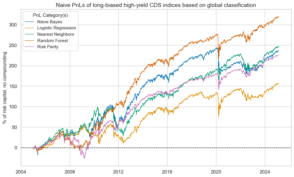
pnls.plot_pnls(
title="Naive PnLs of long-biased high-yield CDS indices based on global classification",
xcat_labels=[
"Naive Bayes",
"Logistic Regression",
"Nearest Neighbors",
"Random Forest",
"Risk Parity",
],
title_fontsize=14,
)
pnls.evaluate_pnls(pnl_cats=["PNL_" + sig for sig in sigx] + ["Long only"])
| xcat | PNL_NB_GLB | PNL_LR_GLB | PNL_KNN_GLB | PNL_RF_GLB | Long only |
|---|---|---|---|---|---|
| Return % | 11.761003 | 7.766294 | 12.286382 | 15.881324 | 11.229509 |
| St. Dev. % | 17.970533 | 17.456844 | 17.493044 | 18.323209 | 14.964405 |
| Sharpe Ratio | 0.65446 | 0.444885 | 0.702358 | 0.866733 | 0.750415 |
| Sortino Ratio | 0.919374 | 0.627657 | 1.018234 | 1.254654 | 1.082005 |
| Max 21-Day Draw % | -59.459877 | -59.459877 | -29.327088 | -59.459877 | -39.639918 |
| Max 6-Month Draw % | -57.168804 | -52.278336 | -57.168804 | -52.278336 | -46.216449 |
| Peak to Trough Draw % | -63.390562 | -63.327214 | -70.537047 | -60.820544 | -58.497244 |
| Top 5% Monthly PnL Share | 0.666926 | 0.839744 | 0.650882 | 0.499943 | 0.612759 |
| USD_GB10YXR_NSA correl | -0.171953 | -0.135708 | -0.172593 | -0.185153 | -0.266613 |
| USD_EQXR_NSA correl | 0.478861 | 0.456983 | 0.464891 | 0.525815 | 0.704258 |
| Traded Months | 243 | 243 | 243 | 243 | 243 |
Vol-targeted positions #
sigx = ["NB_GLB", "LR_GLB", "KNN_GLB", "RF_GLB"]
cidx = cids_cr
pnls = msn.NaivePnL(
df=dfx,
ret="CRXR_VT10",
sigs=sigx,
cids=cidx,
start="2004-12-31",
bms=["USD_GB10YXR_NSA", "USD_EQXR_NSA"],
)
for sig in sigx:
pnls.make_pnl(
sig=sig,
sig_op="raw",
sig_add=0,
sig_mult=1,
rebal_freq="monthly",
rebal_slip=1,
# vol_scale=10,
)
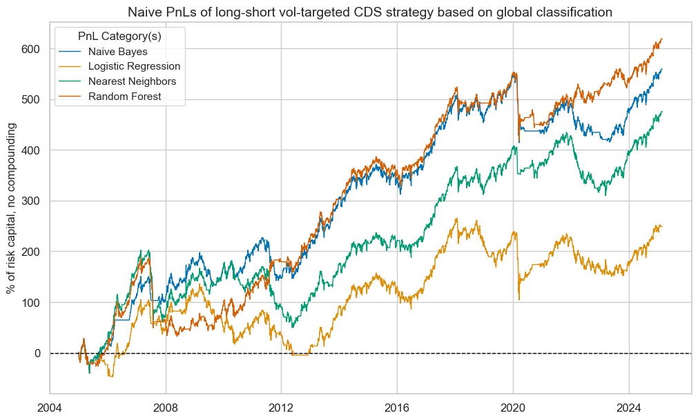
pnls.plot_pnls(
title="Naive PnLs of long-short vol-targeted CDS strategy based on global classification",
xcat_labels=[
"Naive Bayes",
"Logistic Regression",
"Nearest Neighbors",
"Random Forest",
],
title_fontsize=14,
)
pnls.evaluate_pnls(pnl_cats=["PNL_" + sig for sig in sigx])
| xcat | PNL_NB_GLB | PNL_LR_GLB | PNL_KNN_GLB | PNL_RF_GLB |
|---|---|---|---|---|
| Return % | 27.7292 | 12.354446 | 23.566767 | 30.687774 |
| St. Dev. % | 41.950404 | 42.279782 | 42.283466 | 42.102334 |
| Sharpe Ratio | 0.661 | 0.292207 | 0.557352 | 0.728885 |
| Sortino Ratio | 0.923061 | 0.402578 | 0.768317 | 1.007949 |
| Max 21-Day Draw % | -131.548465 | -131.548465 | -99.790888 | -131.548465 |
| Max 6-Month Draw % | -112.129873 | -97.473066 | -136.836688 | -126.658224 |
| Peak to Trough Draw % | -135.27724 | -161.496618 | -153.396012 | -155.734608 |
| Top 5% Monthly PnL Share | 0.57854 | 1.265093 | 0.708539 | 0.535343 |
| USD_GB10YXR_NSA correl | -0.112624 | -0.062484 | -0.104992 | -0.130934 |
| USD_EQXR_NSA correl | 0.385619 | 0.322484 | 0.336628 | 0.39962 |
| Traded Months | 243 | 243 | 243 | 243 |
sigx = ["NB_GLB", "LR_GLB", "KNN_GLB", "RF_GLB"]
cidx = cids_cr
pnls = msn.NaivePnL(
df=dfx,
ret="CRXR_VT10",
sigs=sigx,
cids=cidx,
start="2004-12-31",
bms=["USD_GB10YXR_NSA", "USD_EQXR_NSA"],
)
for sig in sigx:
pnls.make_pnl(
sig=sig,
sig_op="raw",
sig_add=0.5,
sig_mult=1,
rebal_freq="monthly",
neutral="zero",
rebal_slip=1,
# vol_scale=10,
)
pnls.make_long_pnl(vol_scale=None, label="Long only")
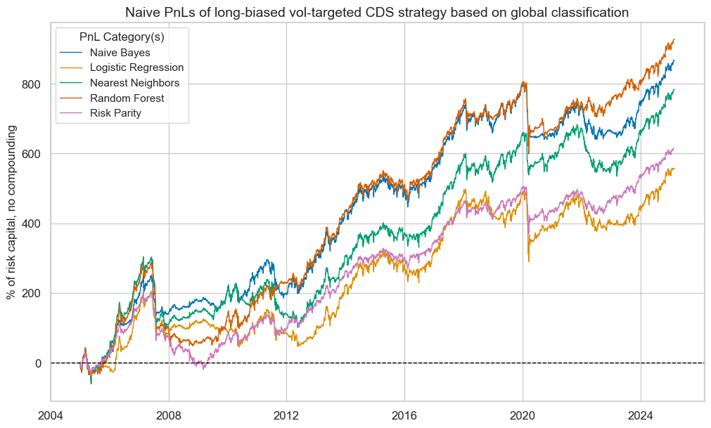
pnls.plot_pnls(
title="Naive PnLs of long-biased vol-targeted CDS strategy based on global classification",
xcat_labels=[
"Naive Bayes",
"Logistic Regression",
"Nearest Neighbors",
"Random Forest",
"Risk Parity",
],
title_fontsize=14,
)
pnls.evaluate_pnls(pnl_cats=["PNL_" + sig for sig in sigx] + ["Long only"])
| xcat | PNL_NB_GLB | PNL_LR_GLB | PNL_KNN_GLB | PNL_RF_GLB | Long only |
|---|---|---|---|---|---|
| Return % | 43.008034 | 27.628583 | 38.845601 | 45.966608 | 30.620536 |
| St. Dev. % | 60.388502 | 58.949964 | 60.693853 | 61.357101 | 44.971252 |
| Sharpe Ratio | 0.712189 | 0.468679 | 0.640025 | 0.749165 | 0.680891 |
| Sortino Ratio | 0.989813 | 0.644445 | 0.881049 | 1.029408 | 0.937405 |
| Max 21-Day Draw % | -197.322698 | -197.322698 | -149.686332 | -197.322698 | -131.548465 |
| Max 6-Month Draw % | -155.153581 | -146.209599 | -205.255032 | -193.352536 | -136.836688 |
| Peak to Trough Draw % | -202.91586 | -209.055207 | -210.521833 | -240.800116 | -222.216642 |
| Top 5% Monthly PnL Share | 0.541493 | 0.818627 | 0.625465 | 0.50274 | 0.532601 |
| USD_GB10YXR_NSA correl | -0.165709 | -0.134411 | -0.160176 | -0.175936 | -0.235164 |
| USD_EQXR_NSA correl | 0.502504 | 0.47159 | 0.467962 | 0.505134 | 0.630778 |
| Traded Months | 243 | 243 | 243 | 243 | 243 |