Boosting macro trading signals

Jupyter Notebook

Boosting is a machine learning ensemble method that combines the predictions of a chain of basic models, whereby each model seeks to address the shortcomings of the previous one. This post applies adaptive boosting (Adaboost) to trading signal optimisation. Signals are constructed with macro factors to guide positioning in a broad range of global FX forwards.
Boosting is beneficial for learning from a wide and heterogeneous set of markets over time, because it is well-suited for exploiting the diversity of experiences across countries and global economic states. Empirically, we generate machine learning-based signals that use regularized regression and random forest regression, and compare processes with and without adaptive boosting methods. For both regression types, machine learning prefers boosting as datasets get larger and, by doing so, creates more profitable signals.

The post below is based on Macrosynergy’s proprietary research. Please quote as “Gholkar, Rushil and Sueppel, Ralph, ‘Boosting macro trading signals,’ Macrosynergy research post, April 2025.”

A Jupyter notebook for audit and replication of the research results can be downloaded here. The notebook operation requires access to J.P. Morgan DataQuery to download data from JPMaQS. Everyone with DataQuery access can download data except for the latest months. Moreover, J.P. Morgan offers free trials on the complete dataset for institutional clients. An academic support program sponsors data sets for research projects.

The basics of boosting and Adaboost

Ensemble methods in machine learning are techniques that combine multiple models to arrive at a single prediction. The aim is to improve accuracy, resilience to noise, and better generalization of the empirical lessons of a specific data sample. The two most common types of ensemble methods are bagging (bootstrap aggregating) and boosting.

• Bagging trains different models on bootstrapped data sets, i.e., random samples of a dataset with replacement, and aggregates results. Aggregation means averaging (for regression) or majority voting (for classification).
• Boosting builds models sequentially such that each model aims to correct the errors of the previous one. Boosting initialises a weak model, for example, a shallow decision tree, and evaluates its prediction errors based on the training data. Then it trains the next model to focus more on those errors. The process repeats over several rounds. In the end, results are aggregated over all models to produce predictions. Unlike bagging, the results of boosted models are weighted based on their training performance.

The theory of boosting says that base models should be “weak learners”. These are models with high bias, e.g., high errors from simplistic assumptions, and low variance, e.g. low errors from sensitivity to changes in the training set. The standard model, therefore, is a linear regression or a shallow decision tree, but boosting can also be applied to multiple weak learners, such as a random forest of stumps.

AdaBoost (Adaptive Boosting) is a standard, popular boosting method that combines multiple weak learners sequentially by adjusting the weights of data points after each model. Here, our focus is on using Adaboost with regressions. The method initializes sample weights as equal shares and trains a first weak model. Based on the training data and predictions of the initial model, sample weights are adjusted in accordance with prediction errors for the training of the next model. The new weight for each sample is calculated by comparing its error with the total training error through a specified “loss function”. The error-based re-weighting and training continue sequentially until the desired number of weak learners has been completed. The prediction of the boosted learners is a weighted median or mean of the weak learners’ predictions. For a more formal explanation, see the paper “Improving Regressors using Boosting Techniques”.

The benefits of boosting for optimizing trading signals

Here we use conceptual macroeconomic factors of a previous post (“Global FX management with systematic macro scores”) to construct optimized trading signals with machine learning. Factors and signals are to be generated for nine developed and 20 emerging market currency areas. The details are given further below.

Generally, machine learning allows sequential macro signal optimization and realistic backtesting (“Macro trading signal optimization: basic statistical learning methods”). Given the limited history of modern financial markets, it is often more effective if one looks at returns and macro factors for a multitude of diverse countries in the form of panel datasets. The process of sequential signal optimization for backtesting and subsequent live trading typically includes three steps:

• Sequential sampling: For each rebalancing date, a so-called “development dataset”t is formed. It consists of panels of candidate trading factors and subsequent returns up to the rebalancing date. This means that development datasets increase with the rebalancing date.
• Model validation: Within each development dataset, candidate prediction models are trained and tested, typically in the form of cross-validation that respects the panel data structure.
• Signal optimization: Based on cross-validation, the best model is chosen for each rebalancing date, its parameters are estimated based on the full development dataset, and its prediction for the next period is used as the “optimized signal”.

For the FX space this process has been shown in previous posts “FX trading signals with regression-based learning” and “How to adjust regression-based trading signals for reliability”. However, it is plausible that boosting will often improve machine learning. That is because the full set of tradable currencies falls into various clusters in terms of geography and characteristics of the underlying economy and monetary policy. This is what econometricians call a “heterogeneous panel”. Similarly, the history of FX forward markets can be divided into “normal” times and various types of crises. Simple models may be dominated by normal times and neglect rare types of crisis.

Adaboost will naturally generate models that focus on underrepresented clusters. Critically, more advanced machine learning methods that reduce variance, such as the random forest, are likely to be biased, due to the heterogeneous panel structure. This results in a high-bias, low-variance model. Boosting is a standard way to improve such models.

Currencies and candidate factors for FX trading signals

In this post, we generate FX forward trading signals for volatility-target positions of 29 smaller currency areas against their natural base currency, i.e., the dollar or the euro, or a basket of the two:

• DM currencies: the Australian dollar (AUD), the Canadian dollar (CAD), the euro (EUR), the Japanese yen (JPY), and the New Zealand dollar (NZD), against the U.S. dollar; the Swiss franc (CHF), the Norwegian krone (NOK), and the Swedish krona (SEK), against the euro; and the British pound (GBP) against an equally weighted basket of dollar and euro.
• EM currencies: the Brazilian real (BRL), the Chilean peso (CLP), the Colombian peso (COP), the Indonesian rupiah (IDR), the Israeli shekel (ILS), the Indian rupee (INR), the Korean won (KRW), the Mexican peso (MXN), the Malaysian Ringgit (MYR), the Peruvian sol (PEN), the Philippine peso (PHP), the Thai baht (THB), the Taiwanese dollar (TWD) and the South African rand (ZAR), all against the U.S. dollar; the Czech koruna (CZK), the Hungarian forint (HUF), the Romanian leu (RON), and the Polish zloty (PLN), against the euro; and the Russian ruble (RUB) and Turkish lira (TRY) against an equally weighted basket of dollar and euro.

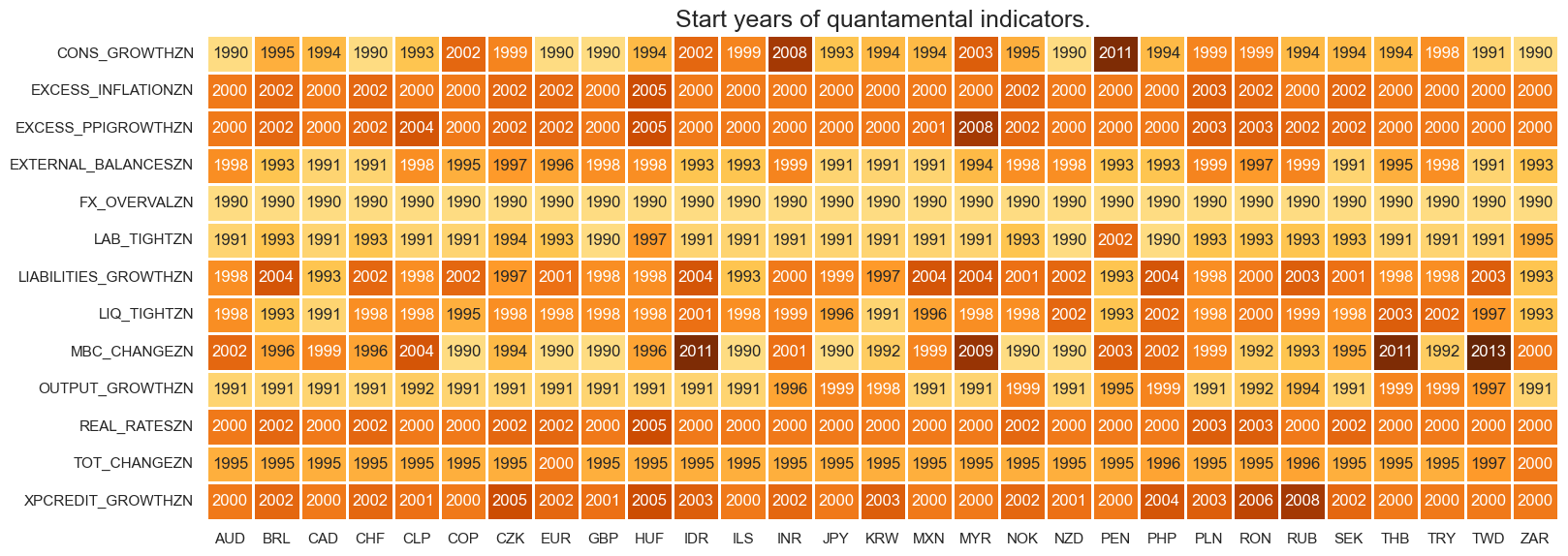
The candidate factors for trading FX forwards have been built based on point-in-time macro-quantamental indicators of the J.P. Morgan Macrosynergy Quantamental System. Macro-quantamental indicators are metrics that combine quantitative and fundamental economic analysis to support investment decisions. Macro-quantamental scores are normalized values of macro-quantamental indicators relative to their (theoretical or empirical) neutral levels, with standard deviations based on a group of similar countries up to the concurrent point in time. Conceptual factor scores are sequentially re-normalized combinations of macro-quantamental scores that measure similar economic concepts, such as economic growth, inflation or external balances.

The specific construction of the 13 candidate conceptual factors has been detailed in the research post mentioned above. Their brief descriptions are as follows:

1. Relative output growth combines four macro-quantamental scores of nowcast GDP and industrial production growth relative to base currency area.
2. Manufacturing business confidence change is based on wo macro-quantamental scores of manufacturing business sentiment changes.
3. Relative labor market tightening uses three macro-quantamental scores of labor market tightening relative to base currency area.
4. Relative private consumption growth is built with four macro-quantamental scores of real consumer spending and consumer confidence relative to base currency area.
5. Relative excess inflation ratio uses five macro-quantamental scores of CPI headline inflation, CPI core inflation, and inflation expectations in excess if the effective inflation target, normalized by target average, and relative to the base currency area.
6. Relative excess credit growth consists of two macro-quantamental scores of private credit growth in excess of the effective inflation target and relative to the base currency area.
7. Real rate differentials and carry combines five macro-quantamental scores of real interest rate differentials and various types of real FX carry.
8. Relative liquidity tightening is measured through four macro-quantamental scores of monetary base and intervention liquidity, relative to base currency area and negative.
9. External balances ratios and changes uses two macro-quantamental scores of external balance ratios and their dynamics.
10. External liabilities growth (negative) is constructed based on two macro-quantamental scores of medium-term accumulation of external liabilities as a ratio to GDP and negative.
11. FX overvaluation (negative) combines three macro-quantamental scores of medium-term depreciation based on purchasing power parity and real effective exchange rates.
12. Relative excess producer price growth uses two macro-quantamental scores of nowcast GDP deflator growth and industrial producer price growth in excess of the effective inflation target and relative to the base currency area.
13. Terms of trade improvement is measured by four macro-quantamental indicators of commodity-based and broader terms of trade improvement.

Relative here means local-currency values minus base currency values. All factor scores have a theoretical positive effect on subsequent local-currency FX forward returns and a theoretical neutral level at zero.

Unfortunately, not all factors are available for all cross sections. India and Indonesia do not provide higher-frequency labour market indicators, and Thailand does not publish a suitable manufacturing business survey. For these two cases, factor scores are imputed as averages of other Emerging Asia countries.

How to apply machine learning and Adaboost for signal generation

Here we apply Adaboost in conjunction with Ridge regressions and random forests to sequential panel-based learning by using the methods of the scikit-learn package and some convenience functions of the Macrosynergy package.

• Ridge regression is a linear regression with regularisation, i.e., with the addition of a penalty term for coefficient size to the regression loss function that prevents the model from fitting the data too closely (view introductory video). Controlling overfitting is very important for macroeconomic time series, economic environments come in global episodes that do not generalize well. A few years data are unlikely to reveal true structural relations. Unlike ordinary least squares, Ridge regression shrinks coefficients in accordance with a squared penalty term on the size of coefficients (called L2 norm). This reduces the influence of individual factors, particularly the dominant ones, but does not remove any of them. This is desirable since all candidate factors have a sound theoretical basis.
  The learning process considers Ridge regression models with and without intercept, and various levels of regularization strength.
• Random forest regression is an ensemble machine learning model that combines multiple regression trees to predict a continuous target variable (view introductory video). It uses bootstrapped samples pf the original dataset to grow a variety of trees. A single regression tree is a decision tree model used to predict continuous outcomes by recursively splitting the data into subsets (view introductory video). Unlike Ridge regression, regression trees detect non-linear and non-monotonic relationships. We have show the application of random forest regression for sequential learning-based trading signals in a previous post (“How random forests can improve macro trading signals”).
  The learning process cross-validates the hyperparameter that controls the amount of feature selection. Larger values impose stronger selection, but reduces the diversity of the forest and vice versa.

We apply sequential signal optimization processes in accordance with the three steps mentioned above and sequential sampling, i.e., model validation and signal optimization to four machine learning pipelines:

• Sequential optimization using Ridge regressions without any boosting.
• Sequential optimization using Ridge regressions with and without boosted versions.
• Sequential optimization using random forest regressions without any boosting.
• Sequential optimization using random forest regressions with and without boosted versions.

The chosen adaptive boosting method are also optimized sequentially, particularly with respect to its learning rate. The learning rate positively affects the variation of the weighted datapoints from one model estimation round to the next. It is well known that boosting is highly sensitive to the choice of learning rate and is consequently a vital hyperparameter to tune.

In sequential optimization, cross-validation is the basis for selecting candidate models and the boosting method. The validation criterion is the implied Sharpe ratio of a binary trading signal based on the stylized trading signals of the test sets (view documentation). It is important to use a suitable cross-validation splitter. Generally, a test estimator has low variance when the test set is large and low bias when the training set is large. For the early short development data sets in sequential optimization, data shortage means that bias reduction is more important than variance reduction. The tradeoff shits as the sample grows.

To manage the bias-variance tradeoff, we use the `ExpandingIncrementPanelSplit` cross-validator of the Macrosynergy package. Each development dataset is split so that subsequent training sets are expanded by a fixed number of time periods to incorporate the latest available information. Each training set is followed by a test set of fixed length (see graph below).

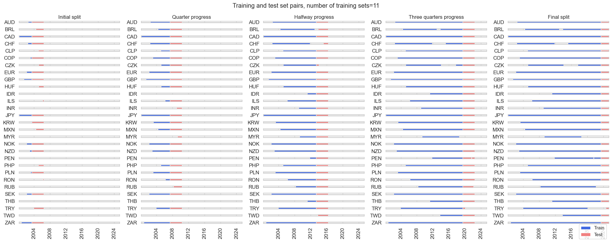
The splitter can be configured such that when limited amounts of data are available, the number of cross-validation folds and the size of test sets are small and the size of training samples is relatively large. As development data sets are expanding, the number of olds and the size of test sets is allowed to grow. For details see the Jupyter notebook.

Empirical evidence of the benefits of Adaboost

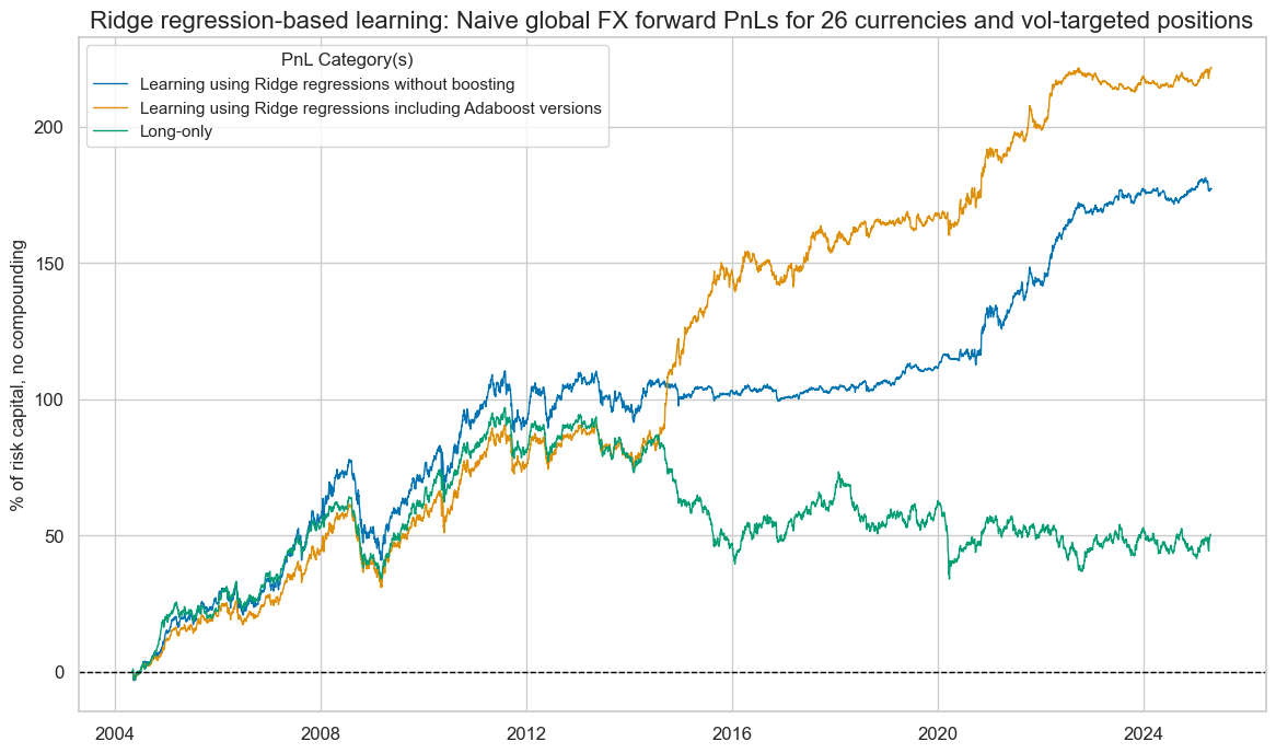
We evaluated the effects of Adaboost, by considering the effects of the various machine learning pipelines on naïve PnLz, based on the various types of optimized signals. Here, the PnL simulation takes vol-targeted FX positions at the beginning of each month in accordance with the optimized signal based on conceptual macro scores at the end of the previous month. We also impose a one-day slippage for positioning change. The simulation does not consider transaction costs and any risk management beyond the volatility targeting.

Machine learning-signal optimization with Ridge regressions that exclude and include boosted learning both show long-term positive value generation. However, the risk-adjusted returns of have been higher if boosting is included, with a Sharpe ratio of 1.1 and a Sortino ratio of 1.6, versus 0.8 and 1.2 for a learning pipeline without boosting. Furthermore, the learning process with boosting showed greater outperformance in the second half of the sample period, as a more extended history was available.

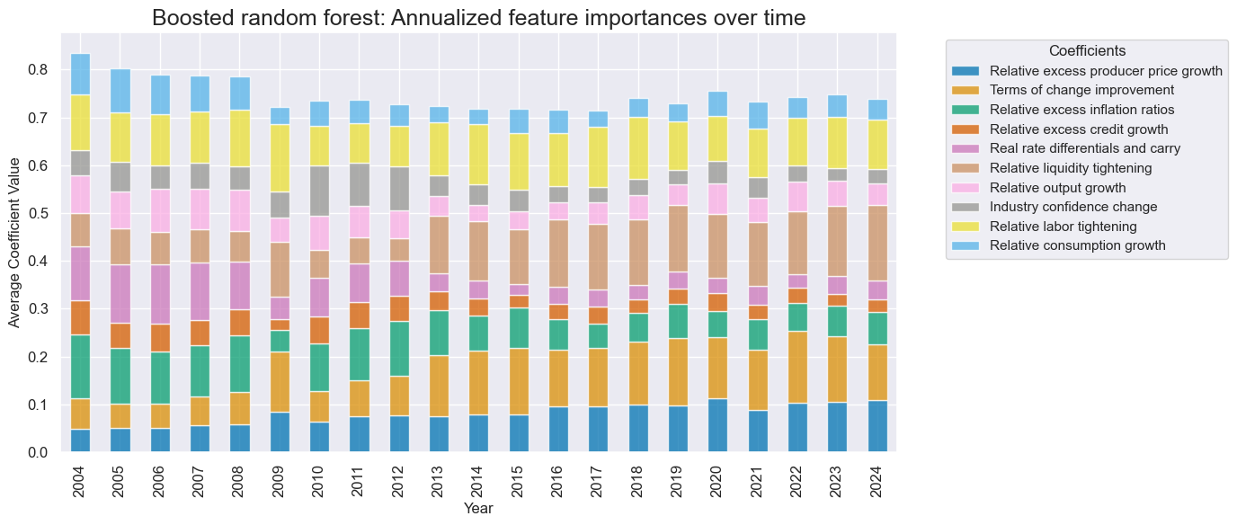
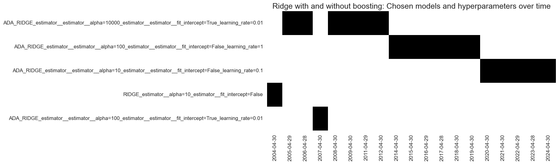
Looking at the chosen optimal models of the inclusive learning pipelines, the graph below shows a clear dominance of boosted models over the past 20 years. Un-boosted models” have only prevailed in the very early years of signal generation.

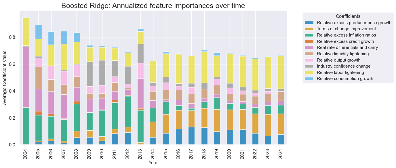
Factor weights of the best signal generation models have naturally converged overtime. Relative labor market tightening, terms-of-trade changes, relative liquidity tightening, relative excess inflation, and relative excess producer price growth have become the strongest influences on predictions.

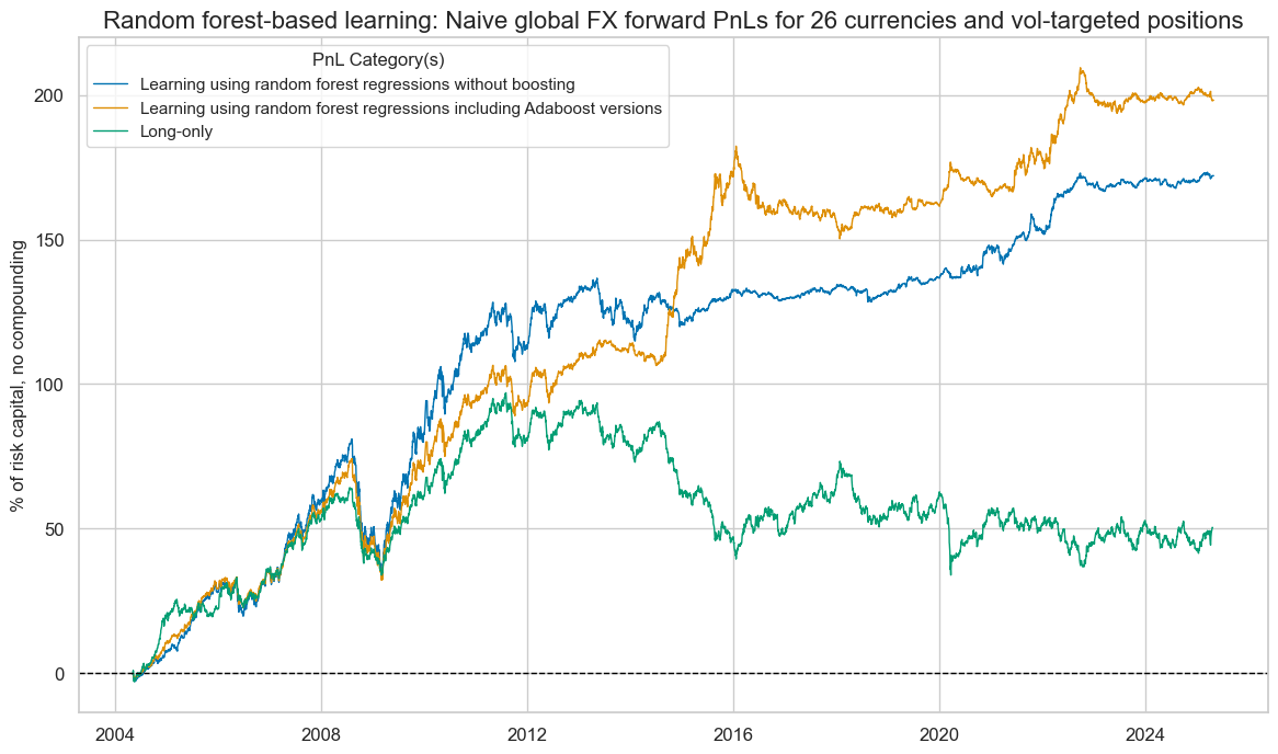
Machine learning-based signal optimization based on random forest regressions echoes the above results. Both signal optimization method, excluding and including boosting, have produced positive PnLs in the long run. However, again, the Sharpe and Sortino ratios of the inclusive process (1.0 and 1.4 ) have exceeded those of the exclusive process (0.8 and 1.4). And again, outperformance of boosting took place only after the first 10 years of the sample. Importantly, the correlation of returns of the inclusive learning signals with equity markets (S&P 500) was just 10% a lot lower than the over 30% for the “un-boosted” signals.

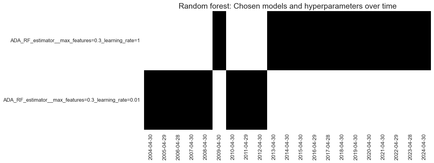
The machine learning process has only ever chosen boosted random forest models since 2004. The models with the highest learning rate have prevailed since the mid-2010s.

Factor weights with random forest regressions are usually more balanced than with standard linear regression methods. However, the most important conceptual factor scores are similar.