Macro trading signal optimization: basic statistical learning methods

Jupyter Notebook

A key task of macro strategy development is condensing candidate factors into a single positioning signal. Statistical learning offers methods for selecting factors, combining them to a return prediction, and classifying the market state. These methods efficiently incorporate diverse information sets and allow running realistic backtests.
This post applies sequential statistical learning to optimal signal generation for interest rate swap positions. Sequential methods update, estimate, and select models over time, adapting to growing development data sets, and apply signals based on the latest optimal model each month. These methods require intelligent choices on model versions, hyperparameters, cross-validation splitters, and model quality criteria. Sequential statistical learning has generally done a good job in discarding irrelevant information and has produced greater accuracy and higher risk-adjusted returns than simple factor averages.

The post below is based on Macrosynergy’s proprietary research and an updated and extended version of a previous article (“Optimizing macro trading signals – A practical introduction”)
Please quote as Gholkar, Rushil and Sueppel, Ralph, “Macro trading signal optimization: basic statistical learning methods”, Macrosynergy research post, March 2025.

A Jupyter notebook for audit and replication of the research results can be downloaded here. The notebook operation requires access to J.P. Morgan DataQuery to download data from JPMaQS. Everyone with DataQuery access can download data, except for the latest months. Moreover, J.P. Morgan offers free trials on the complete dataset for institutional clients. An academic support program sponsors data sets for research projects.

Macro signal optimization and statistical learning

A macro trading signal is a quantitative instruction for positioning in financial contracts based on a systematic process. A trading signal can be composed multiple trading factors, i.e., indicators that predict target returns. The factors themselves must be based on data series that are point-in-time information states of the market or the economy. Both trading signals and factors can be constructed by using empirical evidence or theoretical priors or both. This post focuses on empirical methods that combine theoretical factors into signals through point-in-time optimization, one of the most important tasks in quantitative strategy development. The focus is on macroeconomic factors.

Modern statistical learning offers two great benefits for trading signal optimization.

• First, it can extract information from large amounts of data and can gain insights beyond the cognitive limitations of humans. Not only does statistical learning support the estimation of models (parameters), but it also governs the choice of such models and their structure (hyperparameters), at least within reasonable limits of computation power.
• Second, statistical learning allows realistic backtesting. Rather than choosing factors and models arbitrarily and potentially with hindsight, it simulates a general rational method for making these choices, saving time and diminishing the risks of data or model “mining”.

Statistical learning in macro trading faces one key challenge, however: there is limited evidence on the relationship between key macroeconomic events and relevant financial contract returns. Most liquid derivatives markets have been established only 25-40 years ago. A typical business cycle lasts between 5 and 10 years, while systemic financial crises and macroeconomic regime changes are yet rarer. Certain types of macroeconomic data, such as short-term information state changes and surprises, may have much higher frequency. However, for most purposes, the data on macroeconomic and related financial market experiences are rare and precious. This has two major implications for the optimization of macro trading signals through statistical learning:

• Statistical learning is often more effective if we combine the experiences of multiple countries with diverse experiences in the form of panel data. Using such two-dimensional datasets calls for special cross-validation and hyperparameter optimization methods, as explained below.
• Statistical learning for macro trading signals has a less favorable bias-variance trade-off than other areas of quantitative research. This means that as we give the learning method more freedom, the benefits of reduced bias typically come at the price of much greater model sensitivity to small changes in data, also known as “variance” in machine learning lingo. The steep trade-off reflects the scarcity and seasonality of major macro events and regimes. As a result, it is typically beneficial to concentrate statistical learning on parameters and decisions that cannot be derived from logical or theoretical priors.

Three types of sequential statistical learning

Sequential statistical learning based on panel cross-validation supports signal optimization by tackling three principal tasks:

• Selection of constituent factors of a trading signal from a broader range of factors.
• Selection and application of an appropriate regression method for translating a set of factors into a single return prediction.
• Selection and application of an appropriate classification model to detect favorable or unfavorable regimes for the target returns of a strategy.

This post and the Jupyter notebook demonstrate simple ways to implement these tasks in Python. The machine learning part of the code mainly relies on classes and methods of the scikit-learn package. The code also draws on the Macrosynergy package, mainly its specialized functions for downloading and analyzing macro-quantamental data and its convenience functions for applying scikit-learn to panel data.

All learning tasks for signal optimization rely on the same principle process for sequentially estimating and selecting models (“inner evaluation”) based on point-in-time development data sets and subsequently evaluating the resultant signals (“outer evaluation”). The process has six steps.

1. Specify pandas panel data frames of features and targets at the appropriate frequency. In the features data frame, the columns are indicator categories, and the rows are double indices of currency areas and time periods. The targets are pandas series of (lagged) target returns with the same double index.
2. Define model and hyperparameter grids according to standard scikit-learn conventions. These define the eligible set of model classes and other hyperparameters over which the statistical learning process optimizes. Optimization means periodic model selection based on inner cross-validation and expanding samples.
3. Choose an optimization criterion for sequential model cross-validation, such as accuracy or a Sharpe ratio of stylized PnLs. For macro panel data some of these criteria require special scoring functions of the Macrosynergy package (see section below).
4. Specify time series panel splits for sequential cross-validation using one of the specialized functions of the Macrosynergy package.
5. Perform the actual sequential optimization with the Macrosynergy package’s specialized class (SignalOptimizer). It applies scikit-learn cross-validation to the specific format of macro-quantamental panel data. This optimization compares and chooses models (“inner evaluation”). The sequence of optimal models delivers signals in a standard format and run diagnostics on the stability of the choice of optimal models over time.
6. Evaluate the sequentially optimized signals in terms of predictive power, accuracy, and naïve PnL generation (“outer evaluation”).

Dataset for a practical example

For this post, we optimize a signal for trading 5-year interest rate swaps (IRS) based on daily macroeconomic information from 2000 to March 2025. Target and feature data come from the J.P. Morgan Macrosynergy Quantamental System (“JPMaQS”).

Both features and targets have been taken for 22 developed and emerging economies with liquid interest rate swap markets, which are Australia (AUD), Canada (CAD), Switzerland (CHF), Chile (CLP), Colombia (COP), Czech Republic (CZK), the euro area (EUR), the UK (GBP), Hungary (HUF), Israel (ILS), India (INR), Japan (JPY), South Korea (KRW), Mexico (MXN), Norway (NOK), Poland (PLN), Sweden (SEK), Thailand (THB), Turkey (TRY), Taiwan (TWD), the U.S. (USD), and South Africa (ZAR).

Macro quantamental indicators are distinct from regular economic time series insofar as they present information states, i.e., assign to each date the latest concurrently available value of the indicator. In this way, they are aligned with market price data. We use macro-quantamental indicators to construct four quantamental factors:

• Excess GDP growth: This is the latest estimated GDP growth trend, % over a year ago, 3-month moving average minus a median of that country’s actual median GDP growth rate over the past five years. The latest GDP growth trend is estimated based on national accounts and monthly activity data in the form of sets of regressions that replicate conventional charting methods in markets (view documentation). Excess GDP growth is assumed to predict duration returns negatively, as it indicates a tighter monetary policy stance and higher real returns on capital.
• Excess CPI inflation: This is the difference between information states of consumer price inflation (view documentation) and a currency area’s estimated effective inflation target (view documentation). Consumer price inflation is approximated as the average of a headline and a core CPI growth measure. Excess inflation is assumed to predict duration returns negatively, because it is associated with tighter monetary policy.
• Excess private credit growth: This is the difference between annual growth rates of private credit that are statistically adjusted for jumps (view documentation) and the sum of the currency area’s 5-year median GDP growth and effective inflation target. Excess private credit growth is assumed to predict duration returns negatively because it lessens the need for monetary policy stimulus and indicates risks of exuberant loan demand or supply.
• Excess real yields: This real yield is calculated as the 5-year swap yield (view documentation) minus 5-year ahead estimated inflation expectation according to a Macrosynergy methodology (view documentation) and a presumed neutral benchmark of 1%. Excess real swap yields should predict duration returns positively, as they indicate the drag (or support) of current market conditions on credit demand and investment.

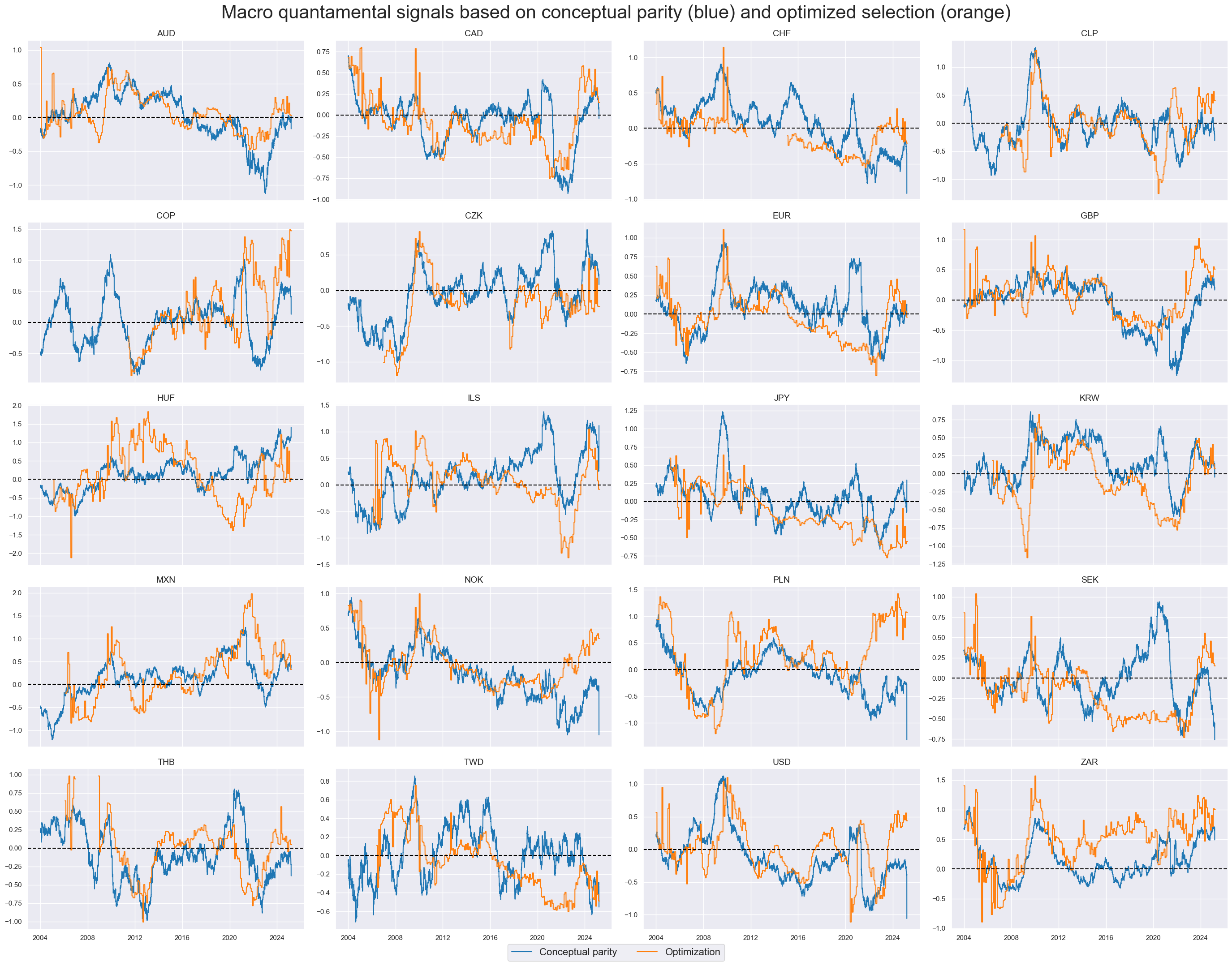
All these factors are sequentially normalized around their presumed neutral level of zero, with extreme values capped at three standard deviations (“winsorization”). The below timeline panel shows the evolution of the factor scores. All are highly autocorrelated and display cyclical dynamics.

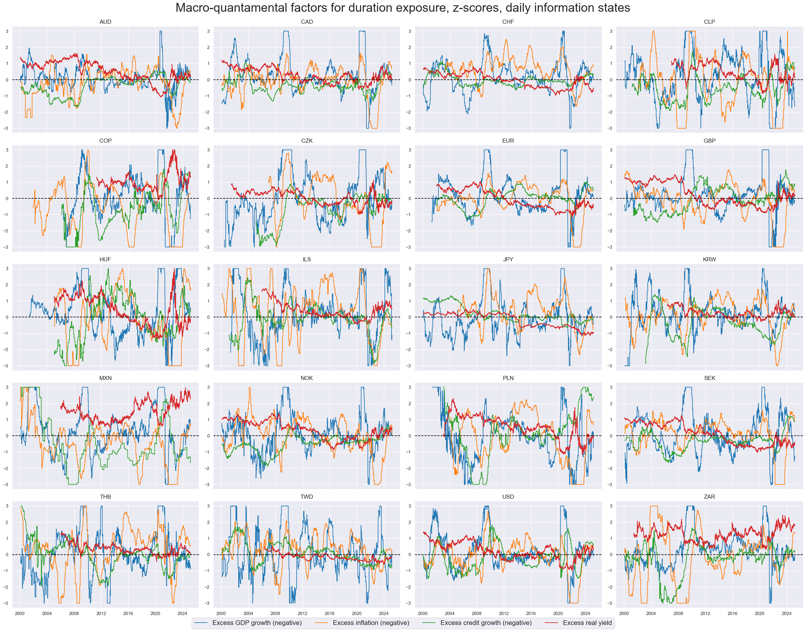
For the purpose of demonstrating the influence of “wrong” pre-selected factors we also simulated four “noise factors” and added them to the statistical learning process. These noise factors autocorrelated quantamental factor scores but are based on random parameters and have no plausible explanatory power regarding duration returns.

The targets of signal optimization are returns on 5-year IRS fixed receiver positions as % of risk capital on positions scaled to a 10% (annualized) return volatility target, and assuming a monthly roll (view documentation). The volatility targeting makes statistical risk comparable across the diverse set of developed and emerging markets.

The benchmark for the success of all optimization exercises below is a simple unweighted composite score of the four normalized indicator categories, each multiplied by the sign of its presumed directional impact. This is also called “conceptual parity”. If factor scores are based on economic theory and strong logic, such a diversified “conceptual parity” benchmark for a wide set of countries is not easy to beat (view related post).

Cross-validation methods

We use cross validation within the expanding development data sets to train and test various model versions regarding their quality of predicting the target returns of unseen data (generalization). Cross-validation splits the development data set into multiple pairs of training and test sets, also called folds. The training data sets are used to estimate the model parameters. The test sets are used to evaluate the estimated models’ performances based on a chosen score. The model with the best score across all folds is then used for signal generation. This process simulates an investor that uses cross-validation at each rebalancing date to select the best model and obtain a signal from this optimal model.

In scikit learn, cross-validation can be implemented through various functions of the model_selection module of scikit-learn, such as cross_validate or cross_val_score. These require a cross-validation splitter that governs the formation of training and test sets. For time series data, there are two popular types of splitting principles:

• Time-series splitting constructs folds by rolling forward in time with an expanding training set and a forward-sliding test set. The TimeSeriesSplit class of scikit-learn produces train/test indices to split samples at fixed time intervals with ascending time indices.
• K-fold splitting builds its folds based on time series blocks of the sample. This splitter would not only predict future data with the past data but also (unseen) past data with the future data. Thus, scikit-learn’s Kfold class produces train/test indices in the form of k blockwise folds (provided `shuffle` is set to False as per default)

None of the standard scikit-learn splitters can be directly applied to panel data of global macro models. Cross-validation splitters for panel data must ascertain the logical cohesion of the training and test sets based on a double index of cross-sections and time periods. It must ensure that all sets are sub-panels over common time spans and respecting missing or blacklisted time periods for individual cross-sections. For this purpose, the Macrosynergy package provides four panel cross validation splitters that are suitable for signal optimization. They are designed to work on double-indexed feature matrices and (lagged) target vectors in the same way as standard sci-kit Learn splitters work on single-index data structures.

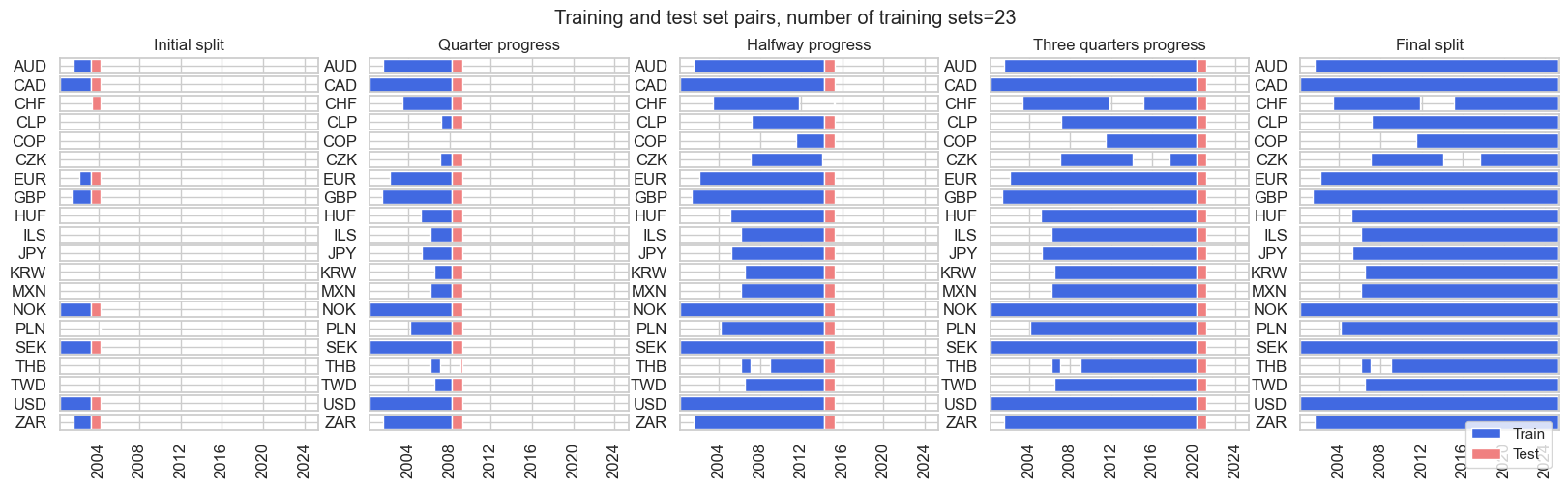
• The ExpandingIncrementPanelSplit class initiates splitters of temporally expanding training panels at fixed intervals followed by subsequent test sets of (typically short) fixed time spans. This simulates sequential learning with growing information sets in fixed intervals.

• The ExpandingKFoldPanelSplit class allows instantiating panel splitters where a fixed number of splits is implemented, but the blocks of panel training sets always precede test sets chronologically and where the time span of the training sets increases with the implied date of the train-test split. It is equivalent to scikit-learn’s TimeSeriesSplit but adapted for panels.

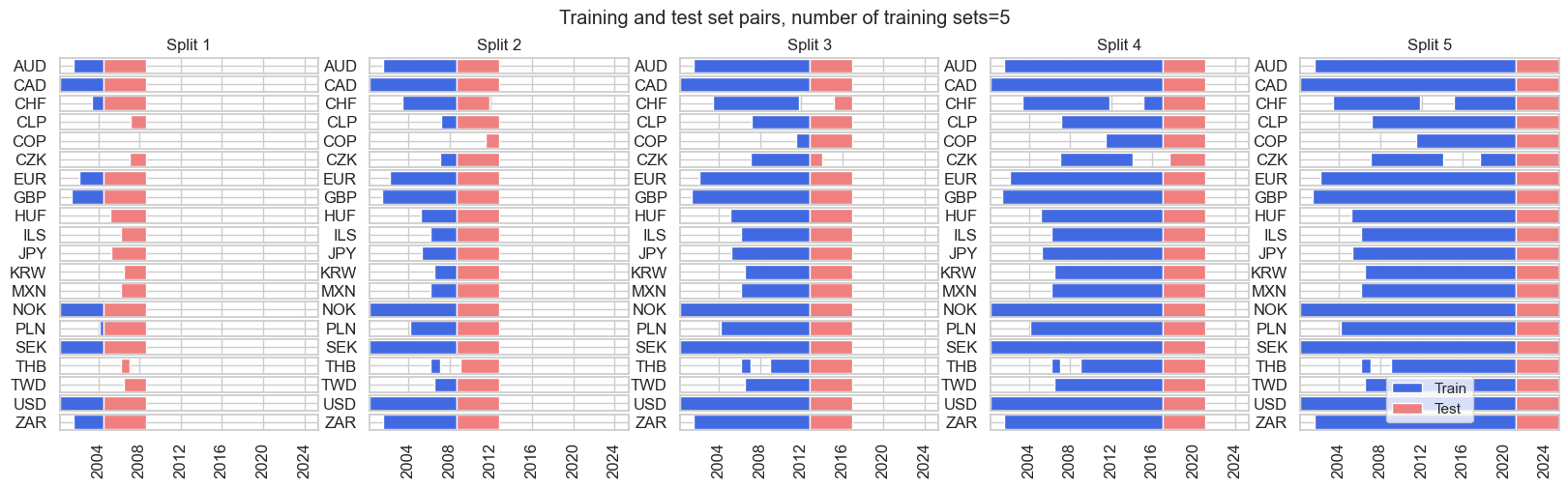
• The RollingKFoldPanelSplit class instantiates splitters where temporally adjacent panel training sets of fixed joint maximum time spans can border the test set from both the past and future. Thus, most folds do not respect the chronological order but allow training with past and future information. While this does not simulate the evolution of information, it makes better use of the available data and is often acceptable for macro data as economic regimes come in cycles. It is equivalent to scikit-learn’s Kfold class but adapted for panels.

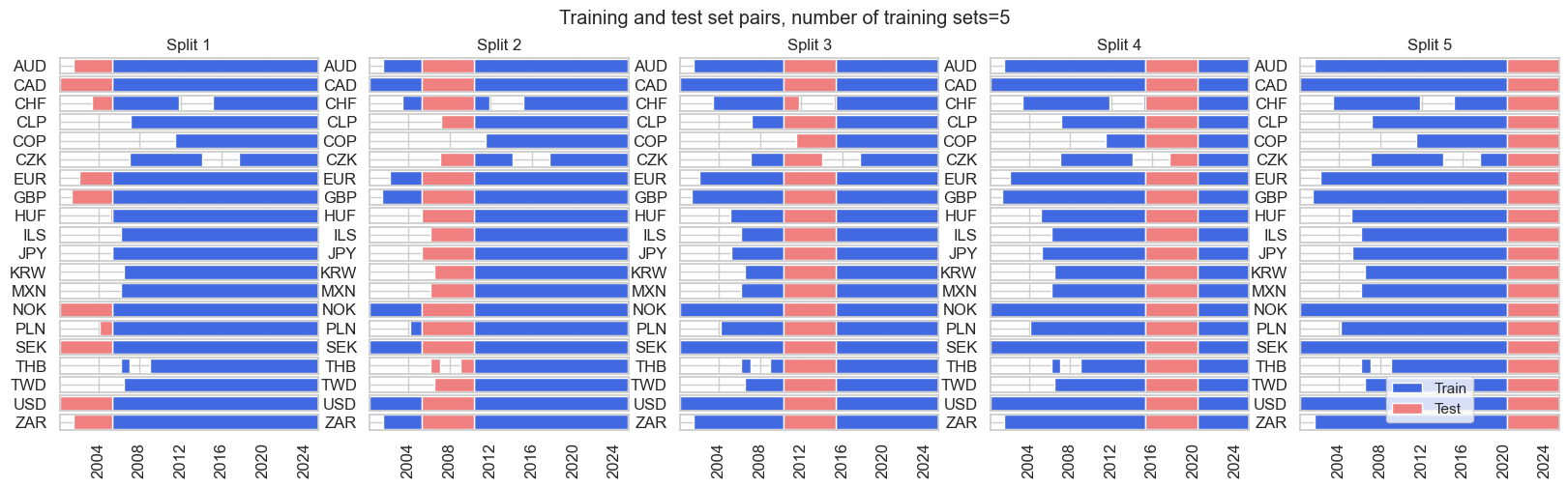
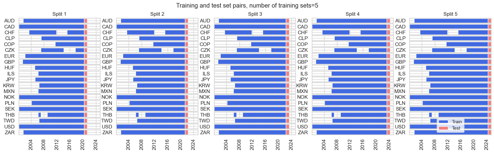
• The RecencyKFoldPanelSplit class is an expanding splitter with test sets concentrated towards the end of the sample period. This prevents very small training sets in initial episodes. When only a single split is specified, this is equivalent to using a single validation set with the most recent data. When multiple splits are specified, the last “n_periods*n_splits” are divided into n_splits equal parts with n_periods being the number of time periods in each validation fold. For a given validation fold, all preceding data is used as the associated training subset.

For the subsequent macro signal optimization examples, we use the RollingKFoldPanelSplit class with four folds since most indicators move in business cycles or at least “mini-cycles”. This means that we need to fully use of development data sets, particularly in the early years.

Optimization criteria

Cross validation requires a performance metric to assess the quality of a model for generalization to unseen data. Popular criteria are R-squared and root mean squared error for regression and AUC-ROC metrics for classification. The Macrosynergy package has added the below criteria that are pariticularly useful for signal generation:

• Panel significance reports the probability of a systematic predictive relation between trading signals and target returns in a panel both cross-sectionally and intertemporally, accounting for correlations between cross-sections in each time period (to avoid the pseudo replication fallacy arising from data pools). The significance probability is based on the Macrosynergy panel test (view post here). It is a criterion that seeks to minimize the risk of accidental relations between signals and returns and can be implemented by the panel_significance_probability method of the Macrosynergy package.
• Naive Sharpe ratio is a measure of risk-adjusted returns of a strategy that uses the sign of the signal for taking subsequent long or short positions across sections and time under the assumption of no trading costs and no risk management. Unlike other criteria, the naïve Sharpe ratio only evaluates the directional accuracy of signals and considers the volatility of a related strategy. It is implemented using the sharpe_ratio method of the Macrosynergy package.
• Naive Sortino ratio is an alternative measure of risk-adjusted returns. While the Sharpe ratio divides annualized returns by annualized standard deviation, the Sortino ratio only divides by negative downside deviations. This avoids penalizing signals that cause occasional outsized positive returns. Some signals are specially crafted for producing high returns in crisis periods. The criterion is implemented by the sortino_ratio method of the Macrosynergy package.
• Correlation coefficients of signals and subsequent target returns are a standard, popular evaluation metric. In the Macrosynergy package, use of the Pearson, Kendall and Spearman rank correlations is made available as performance metrics for cross-validation. Pearson correlation is a measure of linear correlation, whilst the Kendall and Spearman correlations are non-parametric and focus on the communality of the order of observations. All can be implemented by the correlation_coefficient
• Accuracy statistics are handy for the valuation of classification models. Standard accuracy measures the ratio of correctly predicted signs of target returns. It can be implemented with the regression_accuracy For unbalanced samples with predominantly positive or negative return balanced accuracy is more meaningful, i.e., the average ratio of correctly predicted positive and negative returns (regression_balanced_accuracy). A third classification metric is the Matthews correlation coefficient, which condenses the “confusion matrix” that displays all correct and incorrect classifications, into a single number. It is implemented by the regression_mcc method. All three metrics can be applied to panels, by using the respective convenience functions of the Macrosynergy package.

Task 1: Sequentially optimized feature selection

Here, statistical learning chooses the best model for selecting factor scores sequentially at each rebalance date and then applies that model to determine the factor score to be used for the next trading period. Based on this optimal selection, the method calculates an average score. Thus, the optimal signal used at each rebalancing date is an equally weighted mean of the subset recommended by the best model.

For sequential optimized selection (and all other signal optimization methods in this post), features and targets have been converted from daily to monthly frequency by taking the month-end information state of features and the sum of next month’s IRS fixed receiver returns. The monthly frequency is a realistic assumption of how often a trading system would update coefficients and trade on new parameters, balancing the benefits of parameter optimization against transaction costs. Due to the minimum data requirements, optimal model and feature selection produce signals from 2003.

The choice is made over two principal models and a set of model hyperparameters for each.

• The first approach is the Least Absolute Shrinkage and Selection Operator (LASSO). It determines the set of features that have jointly been significant in predicting returns in a linear regression. The LASSO is a regression type that uses “L1 regularization”, i.e., it adds a penalty term to the regression loss function that is linearly proportional to the coefficients’ absolute values. Coefficients of features that display little predictive power are thus shrunk to zero. In scikit-learn, this is implemented through the LassoSelector class of the Macrosynergy package. For macro feature selection, we force all coefficients of presumed positive-impact factors to be positive. This “theoretical prior” ensures that only factors that predict with the theoretically correct sign are considered.
• The second principal approach is the Macrosynergy panel test. It assesses the statistical significance of each factor as return predictors and selects at each rebalancing date those that have individually been significant. Unlike the Lasso, this method evaluates each factor separately, without considering others. It is a simplistic but robust selection process.
  The panel test respects the data structure of features that are indexed by time and cross sections. Simply stacking data for regression leads to “pseudo-replication” and overestimated coefficient significance. This is avoided through panel regression models with period-specific random effects, which adjust targets and features of the predictive regression for common (global) influences (view post here). To apply this test for selection in a scikit-learn pipeline, one can use the MapSelector class of the Macrosynergy package’s learning module.

For both methods, the main hyperparameter is the number of factors to be selected, which can range between 1 and 8. The smaller the number, the more competitive the selection process.

Sequential model selection and optimized signal calculation can be executed by the Macrosynergy package’s SignalOptimizer class. This class uses scikit learn’s GridSearchCV and RandomizedSearchCV and handles the calculation of quantamental predictions based on sequential hyperparameters and model selection. This means it optimizes the selection of the method over the full set of hyperparameter values of the two models. As an optimization criterion, one can use the probability of the significance of the optimized signal in the test sets using the panel_significance_probability score of the Macrosynergy package.

Over time, there has been frequent change across six types of models, particularly in the first five years of optimization. However, with a growing development data set, the learning method preferred panel test and LASSO selectors with two or four factors.

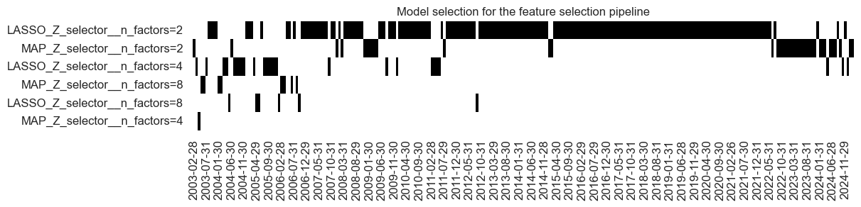
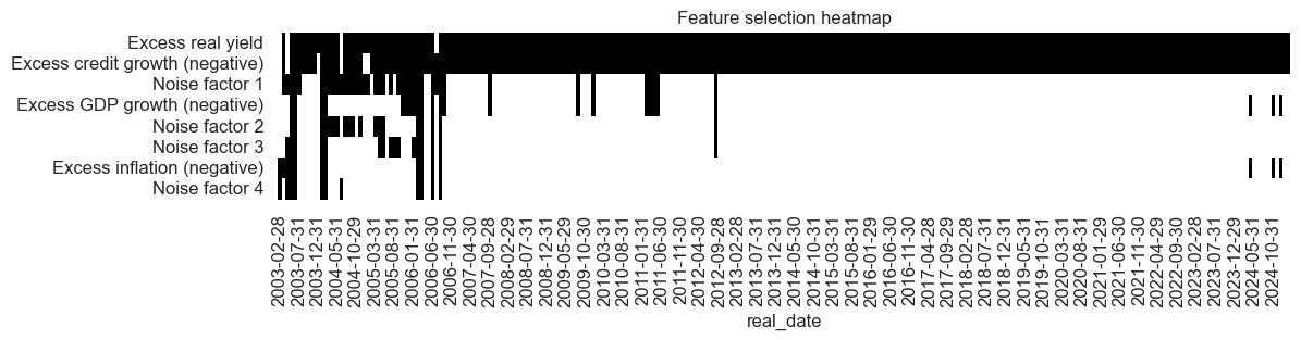
Learning-based selection did a decent job to weed out the noise most of the time, particularly after the first five years. The process selected excess private credit growth and real yields most frequently.

The macro-quantamental signal based on sequentially optimized factor selections has been more volatile and prone to sudden change, when compared to conceptual parity signals. This added volatility reflects changes in models, hyperparameters, and parameter estimates and is one of the drawbacks of sequential optimization. We create a source of signal variation that has no plausible relation to subsequent returns.

Sequential optimization of feature selection has improved the trading signal’s accuracy. For the 22 markets and period 2003-2025 (March), monthly accuracy and balanced accuracy of the prediction of the direction of subsequent returns increased to 54-55% from around 52% for the conceptual parity signal.

To assess the economic value of statistical learning-based signal optimization, we calculate naïve PnLs based on standard rules of Macrosynergy posts: Positions are taken based on optimized and non-optimized feature scores in units of vol-targeted risk in IRS receivers. This means one unit of signal translates into one unit of expected PnL volatility in a specific cross section and holding period. Positions are rebalanced monthly at the beginning of the month based on the last signal at the end of the previous month, allowing for a one-day slippage for trading. The long-term volatility of the PnL for positions across all currency areas has been normalized to 10% annualized, for the purpose of graphic displays. This naïve PnL calculation method does not consider transaction costs or risk management rules, as those are specific to institutional settings.

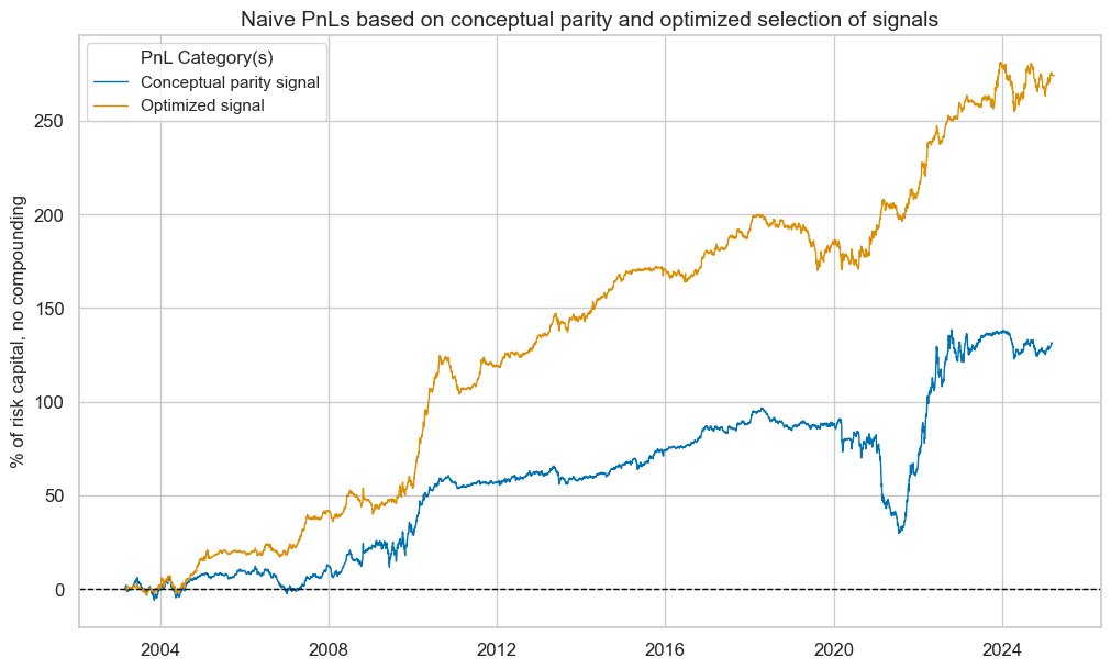
Sequential optimization through selection has improved risk-adjusted returns greatly. The long-term Sharpe ratio of the optimized and parity signals has been 1.2 and the Sortino ratio 1.9, versus 0.6 and 0.8 for conceptual parity. Neither of the two strategies has displayed any meaningful correlation with U.S. treasury returns. The optimization-based signal has been less seasonal and avoided the large drawdown suffered by the parity signal in the 2020s.

Task 2: Sequentially optimized return predictions

The second statistical learning method chooses an optimal prediction method of monthly target returns sequentially and then applies its predictions as signals. Thus, at the end of each month, the method uses the optimized models and parameters to derive a signal for the next month.

To build a grid for sequential optimization, we consider two principal regression models and a set of related hyperparameters:

• The first principal approach is least-squares regression implemented through scikit-learn’s LinearRegression. We use regression with positive coefficient constraints (“non-negative least squares”) to secure theoretically plausible predictive relations. The main hyperparameter that requires empirical validation is the inclusion of the intercept. Conceptually, all features have a neutral level near zero. While this assumption is a bit rough, fitting a constant would bias predictions to the average performance of IRS receiver positions in the training sample, which may be specific to economic and policy conditions.
• The second principal approach is random forest regression implemented through scikit-learn’s RandomForestRegressor class. Random forest regression is an ensemble machine learning model that combines multiple regression trees to predict a continuous target variable. Unlike ordinary least squares, regression trees can model non-linear and non-monotonic relationships. They are also more robust to outliers and accommodate missing data. However, regression trees can easily overfit if not sufficiently “pruned”. See also the post “How random forests can improve macro trading signals.” The main hyperparameter of random forest regression for this post is the ratio of subsample size to draw in bootstrapping relative to the overall panel size to train each tree. A small ration means more diverse but less informed regression trees.

As for feature selection, the sequential model selection and resultant optimized predictions can be executed by the Macrosynergy package’s SignalOptimizer class. The standard optimization criterion for the regression context is the coefficient of determination (R2 score).

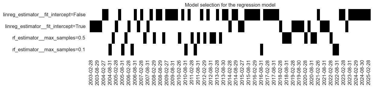
The history of chosen selection models shows usage of both non-negative least squares and random forest regressions, with the simplest and most restrictive model, i.e., non-negative least squares without intercept prevailing in recent years.

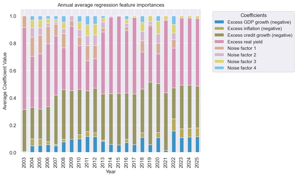
Sequential regression-based learning mostly suppressed the influence of the noise factor and more so as the development data set expanded over time. Excess real yield and private credit growth have become the factors with the greatest weights.

Optimized regression-based predictors show similar medium-term dynamics as the simple feature score averages but also significant differences in average values and short-term dynamics. The average long bias of the optimized prediction has been just under 70%, versus 54% of the conceptual parity score.

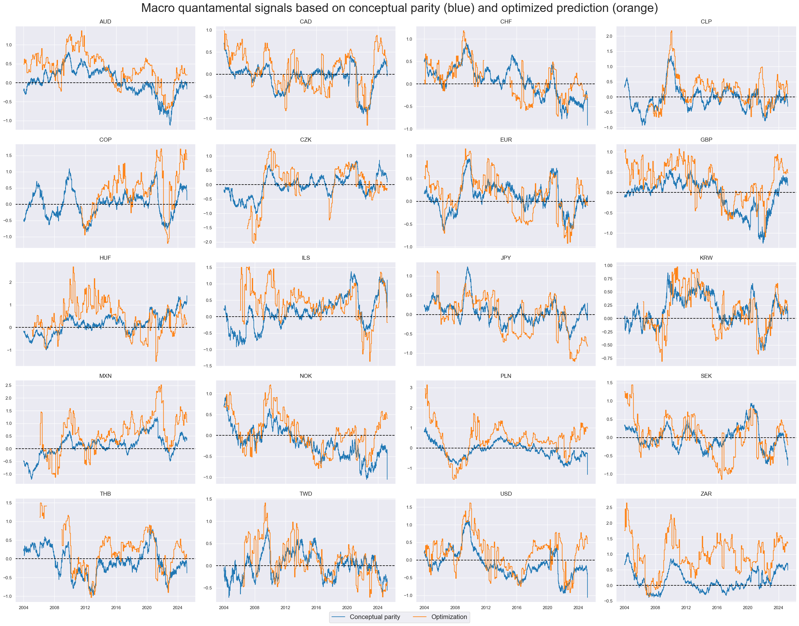
The accuracy and balanced accuracy of the optimized prediction signals were 54% and 53% respectively versus 53% and 52% for the conceptual parity signal.

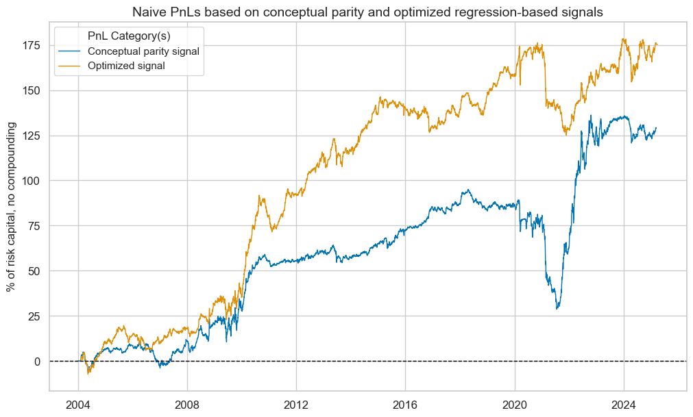
The optimized prediction signal would have produced higher risk-adjusted returns and much less seasonality in PnL generation. The long-term Sharpe and Sortino ratios were 0.8 and 1.2 versus 0.6 and 0.9 for the conceptual parity signal.

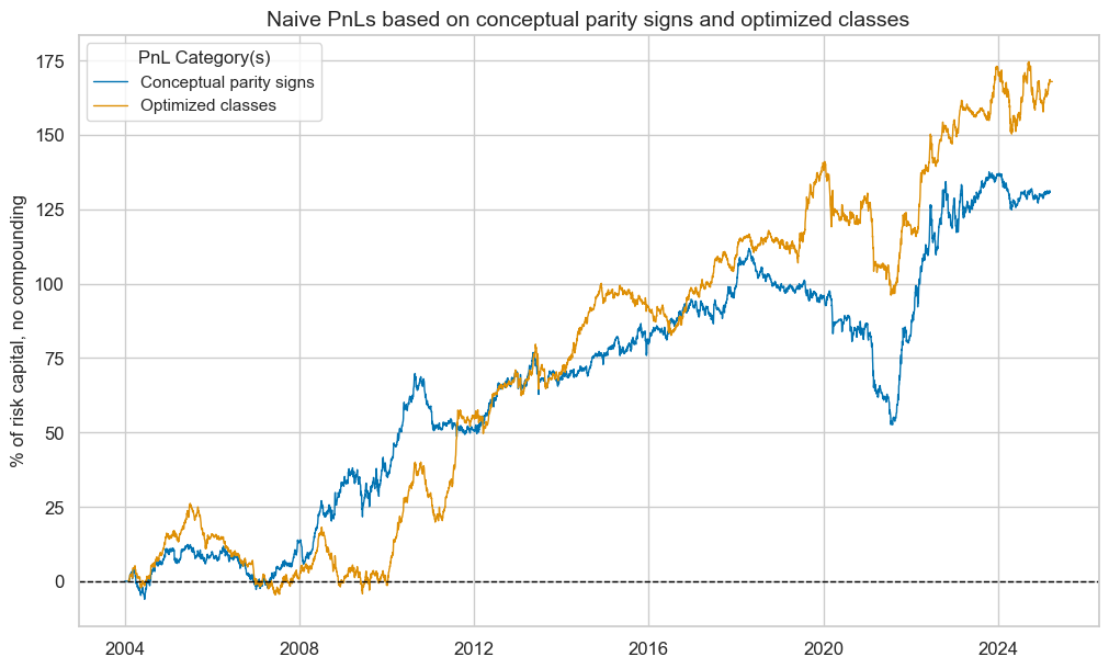
Task 3: Sequentially optimized market classification

The third statistical learning application is the classification of rates market environments into “good” or “bad” with respect to subsequent monthly duration returns. The proposed method chooses an optimal classifier of the direction of market returns sequentially and then applies the class that is predicted by the best classifier, i.e., “positive” or “negative,” as a simple binary trading signal for each currency area.

The hyperparameter grid for this optimization process is based on two conceptually different classification approaches:

• Logistic regression is a popular generalized linear model used for binary classification tasks. It assumes that the probability of a case belonging to the positive class is a logistic function (sigmoid function) of a linear combination of feature values. This implies a linear relationship between the features and the log odds of the probability of the positive class. The odds of an event are defined as the ratio of the probability of a positive outcome to the probability of a negative outcome. In scikit-learn, logistic regression is implemented through the LogisticRegression class. The main hyperparameter that requires empirical validation is the inclusion of the intercept.
• The random forest classifier is an ensemble machine learning, similar to random forest regression. It is implemented through the RandomForestClassifier class in scikit-learn. The main difference is that it uses classification trees, not regression trees and that produces classes through majority voting, rather than values through averaging. As for random forest regression, the main hyperparameter is the subsample  size in bootstrapping

Again, the sequential classifier selection and resultant optimized classifications are executed by the SignalOptimizer class of the Macrosynergy package. The optimization criterion is the Matthews correlation coefficient of the monthly return sign predictions.

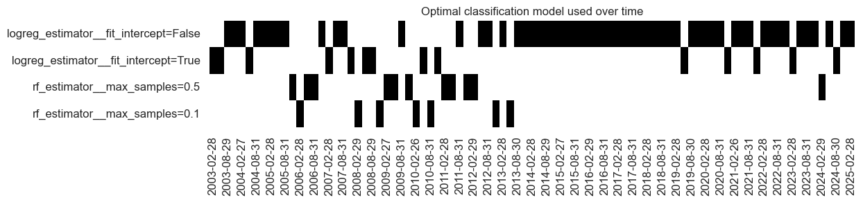
The sequential optimization method reveals a strong preference for logistic regression. As for prediction, the most restrictive model, logistic regression without intercept, has prevailed in recent years.

Optimized classifiers and signs of the conceptual parity signals are mostly equal. Positive or negative regimes can sometimes last for years or even a decade.

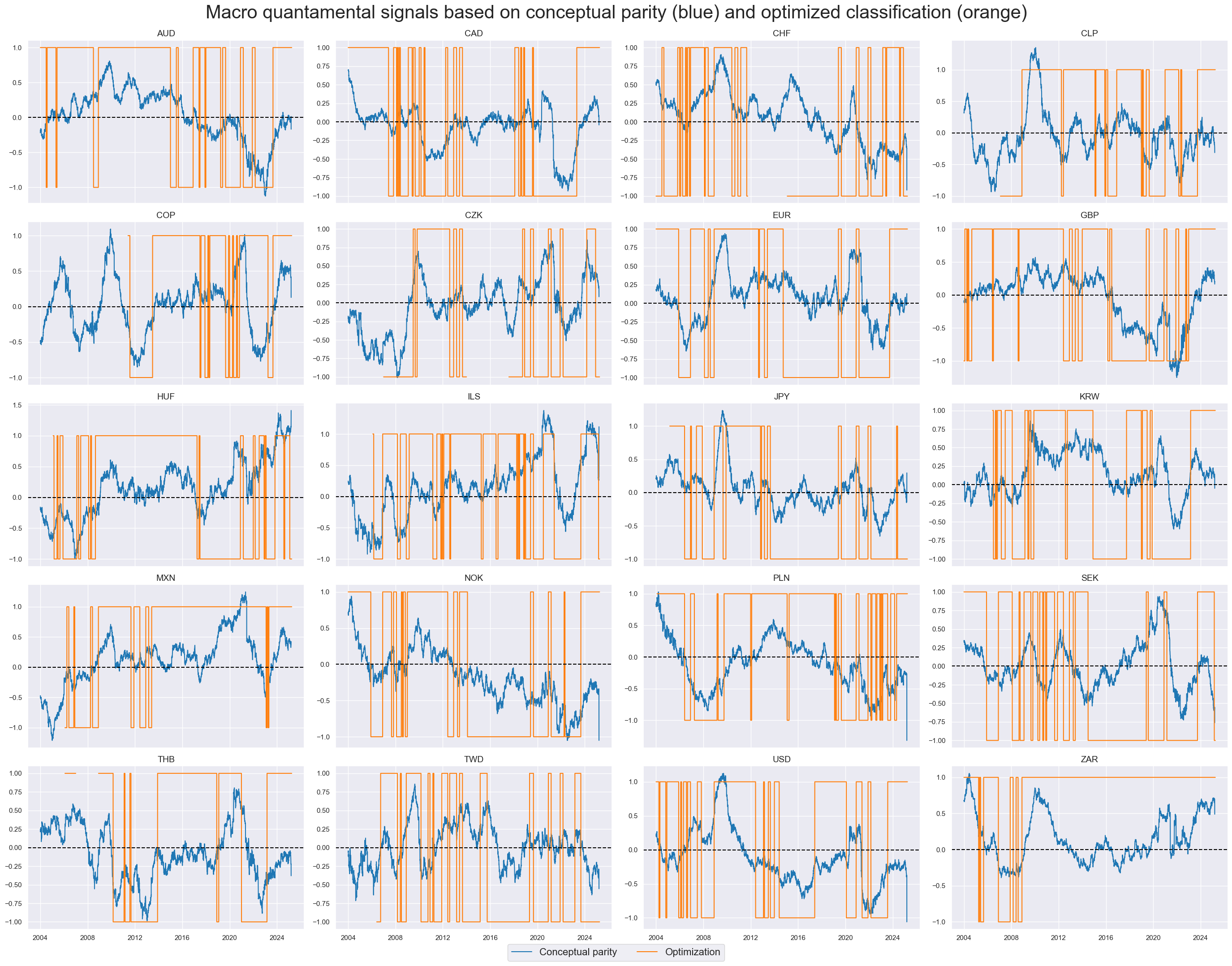
Classification accuracy has been a lot higher with optimized signals than conceptual parity signals. Accuracy and balanced accuracy with statistical learning were 53.8% and 53.3%, versus 52.2% and 51.9% for the conceptual parity signal.

Using binary class signals a naïve PnL shows slightly higher risk-adjusted value for optimized signals versus conceptual parity. The Sharpe and Sortino ratios of the learning signals have been 0.8 and 1.2, versus 0.6 and 0.9 for conceptual parity.