Central banks regularly adjust the economy’s monetary base through foreign exchange interventions and open market operations. Point-in-time information on such intervention-based liquidity expansion has predictive power for asset returns. That is because such operations often come in longer-term trends, and there are lagged effects, for example, through private sector portfolio rebalancing. Alas, the discovery of the economic value of intervention-liquidity signals is often obscured by “ugly backtests”: as a single type of information applied to a single asset type, simulations typically show patchy relevance and uneven value profiles. However, across strategy types and asset classes, intervention-driven liquidity growth has consistently contributed value. A simulation combining two directional and two relative-value strategies demonstrates steady and meaningful PnL generation with low correlation to major market benchmarks.
The post below is based on Macrosynergy’s proprietary research. Please quote as “Sueppel, Elena and Sueppel, Ralph, ‘The (hidden) trading value of central bank liquidity information,’ Macrosynergy research post, August 2025.”
A Jupyter notebook for auditing and replicating the research results can be downloaded here. The notebook operation requires access to J.P. Morgan DataQuery to download data from JPMaQS. Everyone with DataQuery access can download data except for the latest months. Moreover, J.P. Morgan offers free trials on the complete dataset for institutional clients. An academic support program sponsors data sets for research projects.
The importance of central bank interventions for financial markets
Here, interventions are central banks’ transactions in foreign exchange and local securities markets in the pursuit of monetary policy or financial stability objectives. Intervention-driven liquidity expansion refers to the resulting change in the monetary base, which is the sum of physical currency and commercial bank reserves held at the central bank. Growing excess reserves held at the central bank typically fuel the expansion of credit and leverage in the economy. There are two major types of central bank interventions that affect the stock of the monetary base:
- Foreign exchange interventions: With the rise in international capital flows since the 1990s, FX interventions gained prominence as a means to contain exchange rate volatility and to defend target pegs and bands of smaller and emerging economies. Global FX reserves have expanded from under USD 1.4 trillion in 1995 to USD 12.4 trillion by the end of 2024. FX interventions come in two “tastes” depending on their effect on local liquidity: unsterilized and sterilized. Unsterilized interventions purchase foreign currency in exchange for their own base money, thereby expanding the local monetary base commensurately. Sterilized interventions “mop up” the created liquidity through liquidity-draining operations, such as the sale of local-currency bonds.
- Large-scale asset purchase programs: These operations inject base money into the financial system by purchasing various financial assets, including government bonds, agency bonds, corporate bonds, asset-backed securities, exchange-traded funds (ETFs), and real estate investment trusts (REITs). Monetary policy that employs such programs is also known as quantitative easing. Large-scale asset purchase programs became a popular monetary policy tool in the wake of the Great Financial Crisis, after refinancing rates had reached their zero lower bound, and additional support for financial systems and economies could only be provided through non-conventional methods. The programs were primarily run in developed countries, collectively expanding central banks’ balance sheets by over USD 12 billion.
As a result of increased financial market interventions, global central banks’ balance sheets have grown from USD 2-3 trillion in the mid-1990s (about 8% of global GDP) to approximately USD 28 trillion (25% of global GDP) in 2024. This indicates that the influence of central bank interventions on global financial markets has become a major force shaping financial market trends.
In practice, intervention-driven liquidity expansion must be estimated from information provided by the central bank’s balance sheet statements. Here, we use point-in-time estimates of the J.P. Morgan Macrosynergy Quantamental System (JPMaQS). Intervention-driven liquidity expansion or contraction is assumed to have occurred if the sums of the intervention accounts (FX reserves and special purchase accounts) and the monetary base have changed in the same direction over a specific observation period. If intervention accounts and monetary base have moved in opposite directions, intervention liquidity expansion is estimated to be zero. The estimated amount of intervention is the smaller of the absolute change in the intervention accounts and the monetary base. For comparability across currency areas, intervention-based changes are expressed as a percentage of GDP. For some analyses, we compare with simple monetary base expansion, irrespective of market interventions.
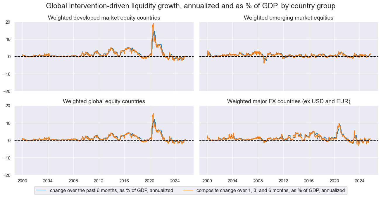
The chart panel below shows the point-in-time information states of intervention-based liquidity expansion for various aggregates. We use multi-horizon expansion rates as % of GDP form JPMaQS, annualize them, and calculate a simple country-level average (documentation here, see also details below). These are then weighted by the local economy’s share of world GDP (in USD) in a specific a global aggregate, here for countries with liquid equity and FX markets (detailed in sections below). In the developed world, particularly in the U.S. and the euro area, this expansion was initially just a minor factor following the “dotcom crisis” in the early 2000s. However, it gained importance in the wake of the 2008/09 global financial crisis and the early 2020s COVID-19 pandemic. In emerging markets and smaller developed countries, intervention liquidity has shown steadier variation.
The extreme seasonality of intervention-based liquidity expansion makes it more challenging to uncover and embrace its trading value. Significant market impact requires large interventions, which are rare events. Related PnL generation based on this factor alone in any single market or position is, therefore, bound to be very uneven, producing “ugly backtests”. However, as shall be shown below, the strong theoretical basis, pervasive empirical evidence, and multiple potential applications of the liquidity expansion factor can make it a significant contributor of risk-adjusted returns in a global macro portfolio.
Why can intervention-related data predict asset returns?
Monetary theory and empirical research suggest that, in isolation and within a low-inflation environment, unsterilized central bank purchases of local assets can reduce interest rate term premiums, compress credit spreads, support equity prices, and mitigate market volatility. Most economists also believe they can at least temporarily reduce the international value of the local currency. Central bank interventions wield their influence on financial markets through three distinct effects:
- Liquidity effect: By increasing the amount of base money in the financial system, central bank interventions increase overall excess reserves held at the central bank. This creates more accommodating funding conditions, encouraging credit supply and financial leverage.
- Portfolio balance effect: When central banks purchase specific securities, they reduce the supply available to private investors. If assets are not perfect substitutes, this can alter relative prices and yields across asset classes, shifting portfolio allocations and risk preferences.
- Signaling effect: Asset purchases can also serve as a communication tool, conveying the central bank’s policy stance or future intentions, such as a commitment to low interest rates. These affect market expectations and behavior accordingly.
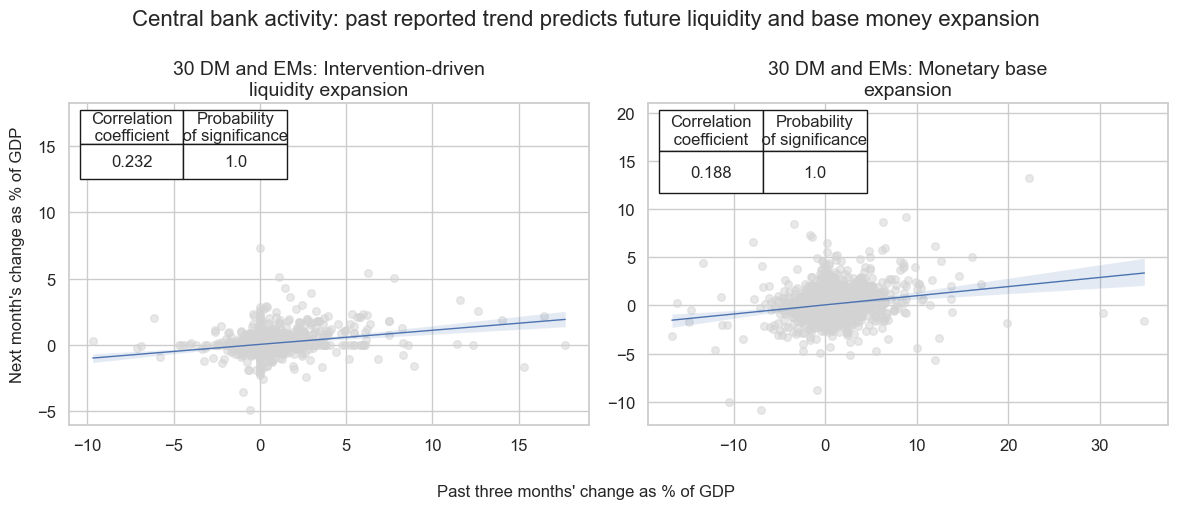
Central bank balance sheet data are typically published 2-4 weeks after the observation period, by which time the liquidity and portfolio balance effect have partly run their course. However, the information should still have predictive power for market trends. Importantly, intervention programs are often implemented over more extended periods. Thus, recent trends should help predict future expansion rates in intervention-driven liquidity. The charts below illustrate the point for both intervention liquidity and monetary base expansion. Information on past expansion rates predicts future reported changes and their variations across currency areas with very high significance and around 20% linear correlation.
Information on intervention liquidity expansion also carries information for other reasons. First, published balance sheets often disclose non-public or unannounced interventions, which have been particularly important in the context of FX market interventions. Second, balance sheets consolidate diverse operations into a unified measure, facilitating cross-country comparisons of purchase volumes and liquidity supply.
This post investigates four simple trading strategies driven solely by intervention liquidity, targeting equity, fixed income, and FX returns. Two are directional strategies: (i) global directional equity and (ii) long–short global duration. The other two are relative-value strategies: (iii) cross-country equity-duration risk parity and (iv) cross-country FX relative value.
Trading a global directional equity index futures basket
The central hypothesis of this trading idea is that liquidity expansion driven by central bank intervention has positive predictive power for equity returns. This effect arises partly from the persistence of intervention activity over time, and partly from the delayed impact of excess reserves created in the process, which eventually fuels demand for real assets.
The target position is an equally-weighted basket of local-currency equity index futures in 19 countries with liquid derivative markets (see documentation). It consists of eight developed and eleven emerging markets. The developed markets are Australia (AUD), Canada (CAD), the euro area (EUR), Japan (JPY), Sweden (SEK), Switzerland (CHF), the United Kingdom (GBP), and the United States (USD). The emerging markets are Brazil (BRL), India (INR), Korea (KRW), Mexico (MXN), Malaysia (MYR), Poland (PLN), Singapore (SGD), South Africa (ZAR), Taiwan (TWD), Thailand (THB), and Turkey (TRY). The specifics of the traded indices are listed in Annex 1.
The single trading factor is a GDP-weighted average of the annualized intervention-based liquidity expansion as a percentage of GDP for all the above countries. The rate of change refers to an average of 1 month, 3 months, and 6 months, i.e., of all three available indicators in JPMaQS (see documentation). GDP weights are based on USD-based point-in-time metrics (see documentation).
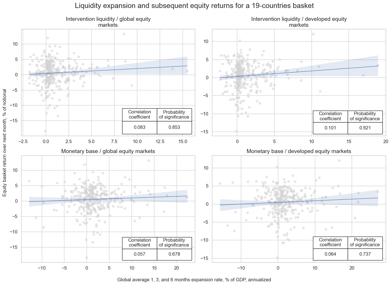
The regression scatter plots below show direction, strength, and significance of the end-of-month liquidity expansion readings with respect to the next month’s equity futures basket returns, for a complete global basket and for the eight developed markets alone. Intervention liquidity growth has been a positive predictor of both basket returns, with 85% and 92% probability of a non-accidental relation for the global and developed market baskets, respectively. Forward correlation was a lot weaker for simple monetary base expansion rates.
Global monthly accuracy, the proportion of correctly predicted directions of subsequent monthly returns, has been just under 60%. This elevated figure is partly attributable to the shared long bias of the signal and equity index futures returns. Nevertheless, balanced accuracy, defined as the average success rate in predicting both positive and negative return directions, has also been strong at 55%.
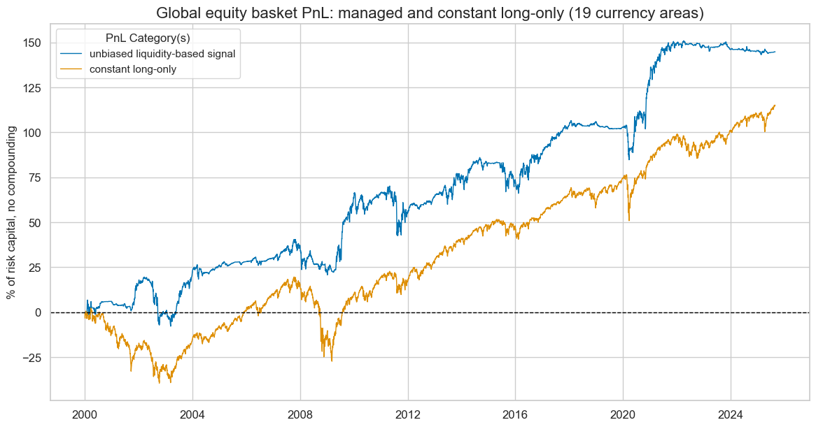
We evaluate value generation using a stylized naïve PnL constructed according to the standard conventions of Macrosynergy research posts. At the end of each month, the strategy derives a trading signal from the normalized value of the global liquidity expansion rate. The normalization uses standard deviations estimated solely from past data, and signals are capped at ±4 to limit the impact of outliers. Positions are adjusted on the first trading day of each month and become effective after one trading day. This naïve PnL does not incorporate transaction costs or risk management rules. For visualization, strategy PnL volatility has been rescaled to 10%.
A simple monthly rebalancing strategy based on an unbiased, normalized trading signal would have achieved a 25-year Sharpe ratio of 0.6 and a Sortino ratio of 0.8 (non-compounded). The strategy has been highly seasonal, generating most of its value during periods of strong liquidity expansion. In this context, seasonality denotes a PnL profile that delivers gains only on relatively rare occasions. For comparison, a constant long-only position over the same period would have produced a lower Sharpe ratio of 0.45 and a Sortino ratio of 0.6. Most importantly, the liquidity-managed strategy exhibited only a 39% correlation with S&P 500 futures returns, versus 93% for the long-only position. This indicates that liquidity-based equity exposure management can provide additive value to passive equity exposure.
Trading a global basket of equity versus duration positions
This strategy is based on the hypothesis that central bank interventions trigger a sequential portfolio rebalancing effect. Since asset purchase programs are conducted primarily in fixed-income markets and only rarely in equity markets, their initial impact should be felt in bonds. Subsequent portfolio rebalancing would then lift equity prices relative to fixed income. In practical terms, following periods of strong intervention-driven liquidity expansion, we would expect local-currency equity returns to outperform local-currency interest rate swap returns on a volatility-adjusted basis.
To implement this effect, we construct a basket consisting of volatility-targeted equity index futures positions and volatility-targeted 5-year interest rate swap positions (see documentation). Risk parity exposure here is a “long-short” position of volatility-targeted equity index futures and volatility-targeted interest rate swap fixed receivers. The basket is built across the same 19 countries used in the equity strategy above. The single trading factor is again the GDP-weighted average of annualized intervention-based liquidity expansion, expressed as a percentage of GDP across all countries.
Over the past 25 years, intervention-based liquidity expansion has been a positive and statistically significant predictor of subsequent monthly equity-versus-duration risk parity returns. This relationship holds for both the global country basket and the subset of developed markets. By contrast, simple monetary base growth has shown considerably weaker predictive power.
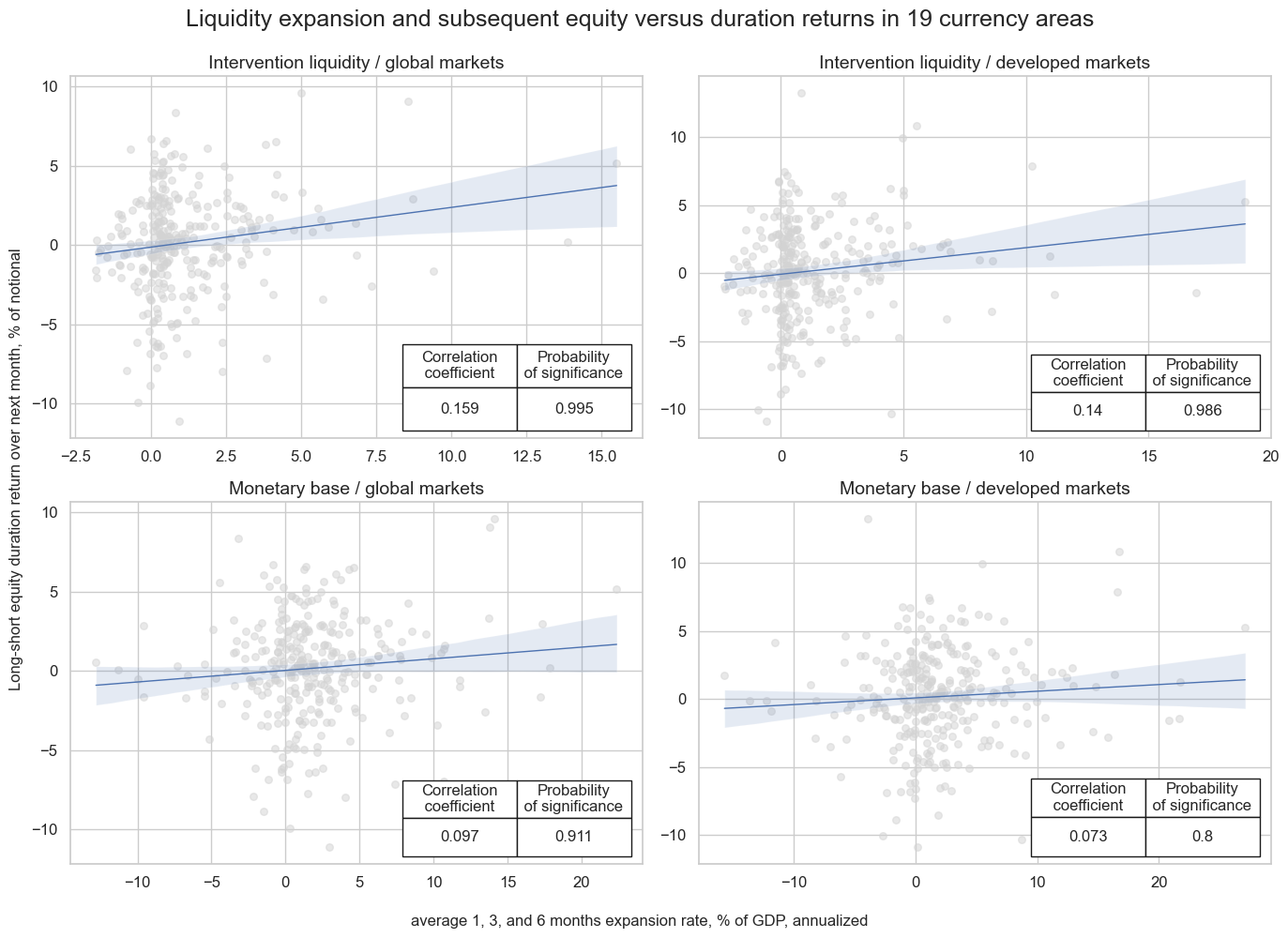
The monthly accuracy of the liquidity expansion signal with respect to the direction of equity versus duration returns has been 60%. Balanced accuracy was just as high; intervention-based liquidity expansion predicted positive and negative returns equally well.
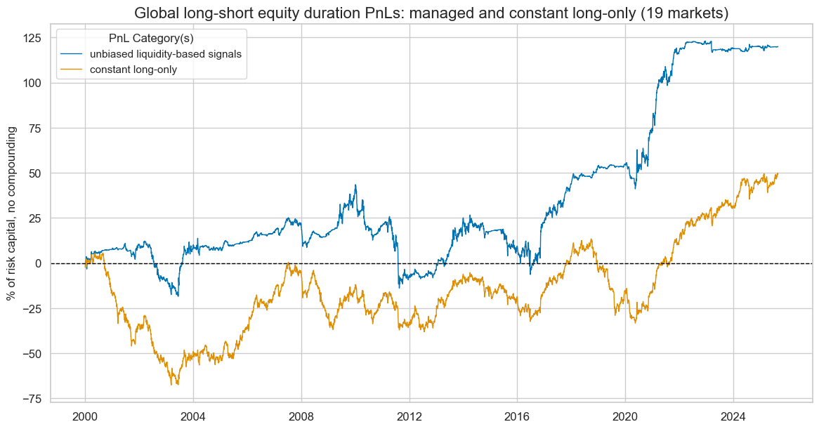
The naïve PnL based on an intervention liquidity score, constructed under the same rules as the equity strategy, has been positive but highly seasonal, with most gains concentrated between 2017 and 2021. Over the full sample, the strategy produced a Sharpe ratio of 0.5 and a Sortino ratio of 0.7. Such pronounced seasonality is not unusual for a single-factor, single-position approach and often limits the appeal of using the signal in isolation. Nevertheless, the theoretical rationale and the robustness of its predictive power support its application, especially when combined with other seasonal indicators.
Trading relative value equity-duration risk parity positions across countries
For diversity of principles, we now shift from global to local intervention liquidity effects. A plausible hypothesis is that the major risk asset classes—equities and duration—tend to perform better in countries experiencing strong central bank liquidity expansion than in those with limited or negative intervention-driven liquidity growth.
Here, positions are local risk parity exposure versus a global multi-country basket of such exposure. Risk parity exposure here is a “long-long” position of volatility-targeted equity index futures and volatility-targeted interest rate swap fixed receivers. The basket consists of the same 19 currency areas that were traded in the above strategies.
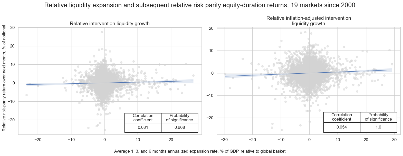
The single trading factor is the average annualized intervention-based liquidity expansion as a percentage of GDP for 1-, 3-, and 6-month lookback horizons relative to a global basket of such rates. Unlike in the above example, there is now one factor per currency area using only the relative local expansion rate. Additionally, to make higher- and lower-inflation countries comparable, we deflate liquidity growth by point-in-time estimates of 1-year-ahead inflation expectations (documentation).
Relative intervention-based liquidity expansion has been positively and highly statistically significant in predicting relative equity-duration “long-long” returns. Inflation adjustment has increased both the strength and significance of the correlation, in line with theoretical reasoning.
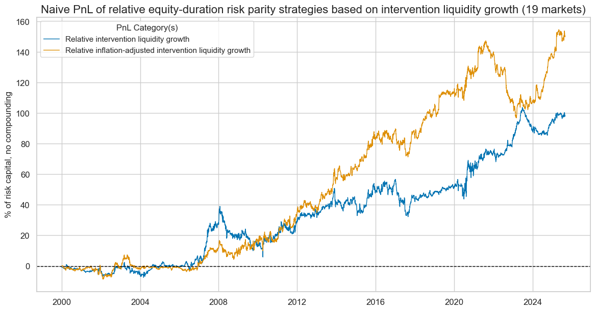
Value generation is again assessed through a naïve PnL. In contrast to the directional strategies discussed above, we do not trade a global basket here but instead construct 19 individual relative positions. Apart from this distinction, the signals and PnL calculation follow the same rules outlined for the directional equity strategy.
The naïve PnL based on the inflation-adjusted relative liquidity expansion has produced material and uncorrelated value. The 25-year Sharpe and Sortino ratios have been 0.6 and 0.8, respectively, with negative or very low correlation to U.S. equity and duration returns. Even without inflation adjustment, the naïve PnL would still have produced long-term Sharpe and Sortino ratios of 0.4 and 0.55, with near-zero correlation to equity and fixed income benchmarks. Seasonality is high, as this is still a single-principle macro strategy. Particularly, there was little value generation in the early 2000s, prior to the rise of non-conventional monetary policy.
Trading FX forwards relative to baskets
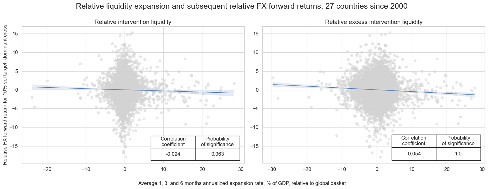
Finally, we apply signals based on relative intervention-based liquidity expansion to FX forward trading. The basic hypothesis is straightforward: currencies with high central bank liquidity growth in their respective economic areas are expected to underperform, reflecting easier monetary policy and the accumulation of financial institutions’ excess reserves.
- This strategy can be applied to FX forwards of 27 “smaller” currency areas, whereby smaller here means eight developed markets excluding the U.S. and the euro area, and 19 emerging markets. Specifically, the traded developed market exchange rates are (in order of local currency tickers): the Australian dollar (AUD), the Canadian dollar (CAD), the euro (EUR), the Japanese yen (JPY), and the New Zealand dollar (NZD), against the U.S. dollar; the Swiss franc (CHF), the Norwegian krone (NOK), and the Swedish krona (SEK), against the euro; and the British pound (GBP) against an equally weighted basket of dollar and euro.
- The EM forwards trade the following exchange rates: the Brazilian real (BRL), the Chilean peso (CLP), the Colombian peso (COP), the Indonesian rupiah (IDR), the Israeli shekel (ILS), the Indian rupee (INR), the Korean won (KRW), the Mexican peso (MXN), the Malaysian Ringgit (MYR), the Peruvian sol (PEN), the Philippine peso (PHP), the Thai baht (THB), the Taiwanese dollar (TWD) and the South African rand (ZAR), all against the U.S. dollar; the Czech koruna (CZK), the Hungarian forint (HUF), the Romanian leu (RON), and the Polish zloty (PLN), against the euro; and Turkish lira (TRY) against an equally weighted basket of dollar and euro.
Historical periods when exchange rates were pegged or forwards untradable are excluded by using point-in-time indicators of these conditions from JPMaQS (documentation). FX forward positions for all trades are vol-targeted for an expected 10% annualized standard deviation of returns in order to avoid risk concentration in the most volatile exchange rates (documentation).
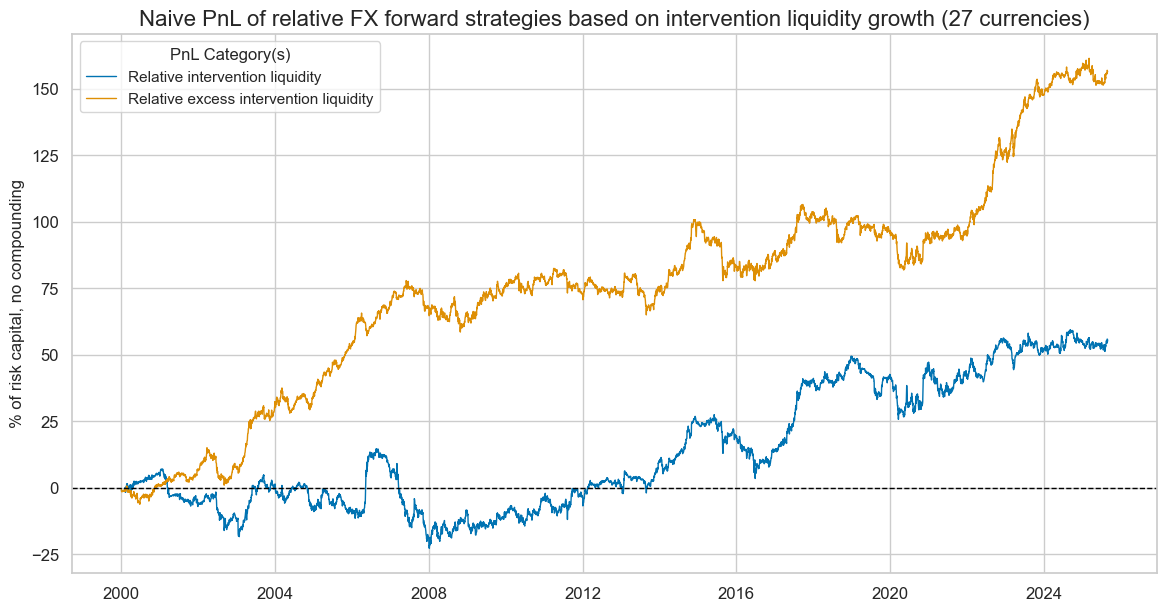
As before, the trading factor is the local intervention-based liquidity expansion over multiple horizons relative to the cross-area average. Additionally, the focus is again on an inflation-adjusted version of liquidity growth, since the set of currency areas considered is highly diverse in terms of inflation expectations. As expected, relative liquidity expansion has negatively and significantly predicted subsequent relative monthly FX forward returns. The predictive relationship was stronger and more significant for the inflation-adjusted relative liquidity expansion signal.
Risk-adjusted value generation, as measured by a naïve PnL, has been material since 2000, albeit only for the inflation-adjusted liquidity metrics. The long-term Sharpe and Sortino ratios have been 0.8 and 1.2, respectively, with less seasonality than other purely liquidity-driven strategies. There has been some modest (20%) correlation with the S&P500. Without inflation adjustment, FX RV trading would only have produced a little risk-adjusted return overall and no value prior to the Great Financial Crisis.
Combined trading value of liquidity expansion
All of the above strategies produced highly uneven and seasonal PnLs, which may seem modest or unattractive in isolation. However, such seasonality is typical of single-principle macro strategies, since the underlying macroeconomic phenomenon must actually materialize for the strategy to generate value. Moreover, within each asset or asset class, the factor must compete with numerous other drivers. In essence, a single macro factor can only add value to a set of contracts when it becomes the dominant influence—an inherently occasional occurrence.
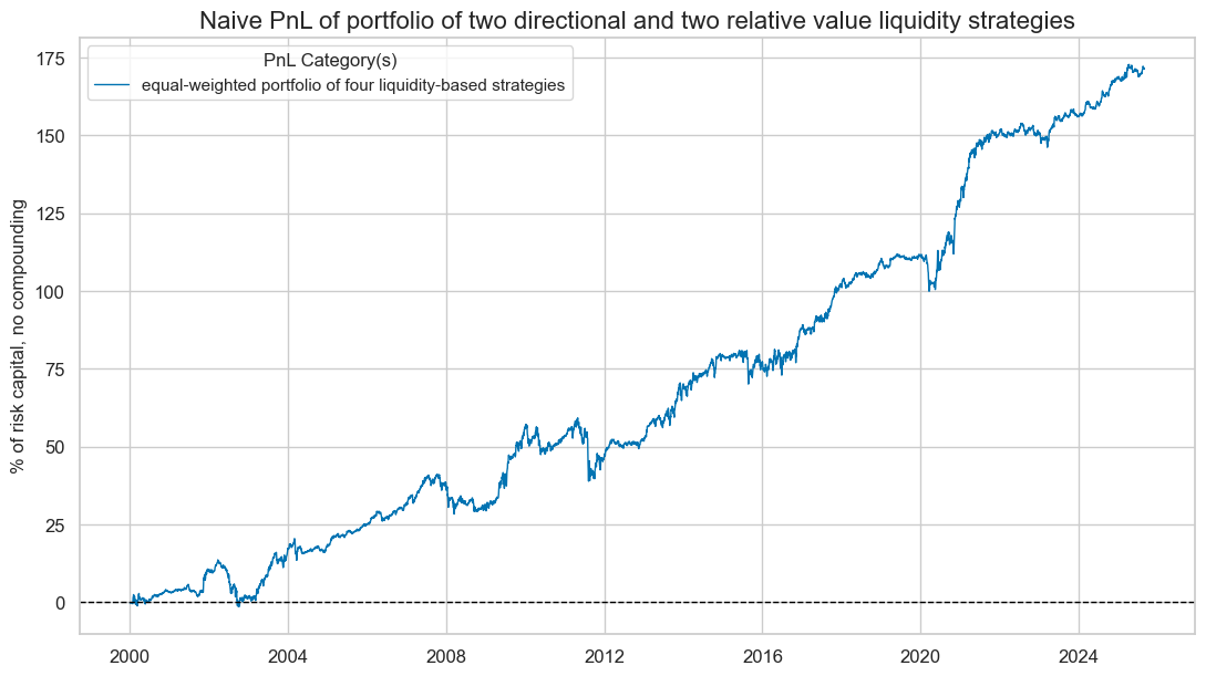
However, when combining the PnL generated by liquidity-based signals across different strategies, a more pervasive value generation comes to the fore. The below naïve PnL is a composite of the four above strategies. For this purpose, each strategy has been given stable leverage so as to keep long-term annualized volatility around 10-15%. Then, the four PnLs are simply aggregated to a single cross-strategy PnL.
The naive PnL of this aggregated strategy has been considerably less seasonal than the individual PnLs. The 25-year Sharpe and Sortino ratios have been 1.0 and 1.5 before transaction costs, with 32% correlation with the S&P500 returns. The 5% most profitable months accounted for about half of the overall PnL value, which is not excessive for a macro strategy.
When excluding the two directional strategies, the aggregate PnL of the two relative value strategies still would have produced material, consistent, and uncorrelated positive returns. The long-term Sharpe and Sortino ratios of the two RV strategies have been 1.1 and 1.7, and the correlation with the S&P500 has been just 5%.
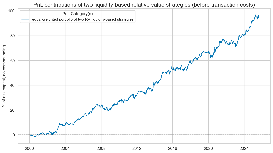
This highlights an important point: a set of individually modest but diverse strategies based on the same macro factor can combine to generate material and durable value.
Annex 1
This post looks at eight developed market local-currency index futures and eleven emerging market local-currency index futures. The developed market indices are (in alphabetical order of currency symbol):
- AUD: The S&P/ASX 200 is the primary index for the Australian equity market. It measures the performance of the 200 largest companies by market capitalization listed on the Australian Stock Exchange (ASX).
- CAD: The S&P/TSX 60 Index is designed to represent the large-cap segment of the Canadian equity market. It includes 60 of the largest and most liquid companies listed on the Toronto Stock Exchange (TSX).
- CHF: The Swiss Market Index (SMI) is Switzerland’s premier stock market index, representing the 20 largest and most liquid companies listed on the SIX Swiss Exchange.
- EUR: The EURO STOXX 50 Index is a leading stock market index for the euro area, representing the 50 largest and most liquid blue-chip companies from 11 Eurozone countries.
- GBP: The FTSE 100 Index is a stock market index representing the 100 largest publicly listed companies by market capitalization on the London Stock Exchange (LSE).
- JPY: The Nikkei 225 Stock Average Index is a prominent stock market index in Japan, representing 225 of the largest and most liquid companies listed on the Tokyo Stock Exchange (TSE).
- SEK: The OMX Stockholm 30 (OMXS30) Index is a major stock market index in Sweden, representing the 30 most traded large-cap companies listed on the Nasdaq Stockholm exchange.
- USD: The S&P 500 Composite Index is one of the most widely followed stock market indices in the world, representing 500 of the largest publicly traded companies in the United States. (Note that even though the U.S. is about twice the size of the euro area, the market capitalization of the S&P500 has been roughly ten times that of EURO STOXX.)
The emerging market indices are:
- BRL: The Brazil Bovespa Index, also known as the Ibovespa is the main stock market index in Brazil, representing the performance of the most actively traded companies on the B3, the São Paulo Stock Exchange.
- CNY: The Shanghai Shenzhen CSI 300 index is a benchmark in China that tracks the 300 largest and most liquid A-share stocks traded on the Shanghai Stock Exchange (SSE) and the Shenzhen Stock Exchange (SZSE).
- INR: The CNX Nifty (50) is the flagship stock market index of the National Stock Exchange of India. It represents the weighted average of 50 of the largest and most actively traded stocks spanning 13 sectors of the Indian economy.
- KRW: The KOSPI 200 Index is a major stock market index in South Korea, representing the performance of the 200 largest and most liquid companies listed on the Korea Exchange (KRX).
- MXN: The Mexico IPC, often referred to as the Bolsa Index, is the main stock market index in Mexico. It tracks the performance of the 35 largest and most liquid companies listed on the Mexican Stock Exchange.
- MYR: The FTSE Bursa Malaysia KLCI (Kuala Lumpur Composite Index) is the main stock market index in Malaysia. It tracks the performance of the 30 largest companies by market capitalization listed on the Bursa Malaysia
- PLN: The Warsaw General Index 20 comprises the 20 largest and most liquid companies listed on the Warsaw Stock Exchange (WSE) in Poland.
- SGD: The MSCI Singapore (Free) Index represents the performance of the Singapore equity market through a free float-adjusted market capitalization-weighted index.
- THB: The Bangkok SET 50 Index is a major stock market index in Thailand, representing the 50 largest companies listed on the Stock Exchange of Thailand.
- TWD: The Taiwan Stock Exchange Weighted Index (TAIEX) is the main stock market index in Taiwan. It tracks the performance of all listed companies on the Taiwan Stock Exchange.
- TRY: The BIST 30 Index is one of the leading stock market indices of Turkey, tracking the 30 largest and most liquid companies listed on Borsa Istanbul.
- ZAR: The FTSE/JSE Top 40 Index is a key stock market index in South Africa, representing the 40 largest companies listed on the Johannesburg Stock Exchange (JSE) by market capitalization.


