The popularity of trend-following bears the risk of market excesses. Medium-term market price trends often fuel economic trends that eventually oppose them (”macro headwinds”). Fortunately, relevant point-in-time economic indicators can provide critical information on the sustainability of medium-term market movements and are a natural complement to standard trend signals.
This post illustrates the benefit of combining market and macro trends in equity markets. Since the 1990s, “robust” market price trend signals alone have created value for equity index future strategies in developed markets. However, risk-adjusted returns would have been enhanced materially if one adjusted market signals for natural macro headwinds, such as the state of the business cycle, inflation, and equity valuations.
The post below is based on Macrosynergy’s proprietary research. Please quote as “Cereda, Fabio and Sueppel, Ralph, ‘Equity trend-following with market and macro data,’ Macrosynergy research post, May2025.”
A Jupyter notebook for audit and replication of the research results can be downloaded here. The notebook operation requires access to J.P. Morgan DataQuery to download data from JPMaQS. Everyone with DataQuery access can download data except for the latest months. Moreover, J.P. Morgan offers free trials on the complete dataset for institutional clients. An academic support program sponsors data sets for research projects.
Market trends and macro headwinds
Market trends are a popular and century-old guide for trading. Trend-following sets positions in accordance with specific metrics of past price changes or return trends. There is ample empirical evidence and theoretical reason for the persistence of market trends. They result from the gradual dissemination of information, disposition effects (a tendency to sell profitable positions and hang on to loss-making positions), rational herding (a conscious decision to mimic the actions of other market participants), and lazy trading (sluggish position adjustment due to information and transaction costs). However, traditional market trend-following gives no consideration whatsoever to fundamental developments. This means that the growing popularity of trend-following over the past decades increases the risk of market excesses and thus may become self-defeating.
The plausible antidote to excesses in market trends is tracking economic developments. The main idea is that persistent market trends will eventually invite opposing macroeconomic developments, a phenomenon also called the “macro headwind theory”. A macro headwind is defined as an economic development that undermines prevailing medium-term market price trends. Conversely, a macro tailwind is a development that supports current market trends. For example, by themselves, positive currency trends tend to erode an economy’s competitiveness. In the equity space, rising stock prices boost household wealth and corporate investment. The resulting addition to domestic demand increases economic growth, reduces labor market slack, and ultimately exerts inflationary pressure, all of which call for tighter monetary policy and higher real interest rates, reducing the net present value of future dividend flows.
The consideration of macro trends should make the market-trend signals more robust to excesses and benefit long-term value generation. Specifically, point-in-time relevant macro trends inform on the sustainability of market trends. As a result, incorporating macroeconomic information alongside price trends can provide a better-informed overall signal.
Robust market trends
To represent equity index future trends in this post, we use Tzotchev’s (2018) robust trend-following method (view paper). It calculates signals based on past average market returns divided by their estimated standard deviation (“t-statistics”) for various lookback horizons. These statistics are indicative of the probability of a past negative or positive return trend being significant. Furthermore, volatility-adjusted average returns can be translated into intuitive signals within a range of -1 to +1, by using the following formula:
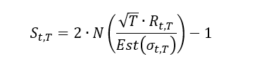
whereby
- St,T is a signal calculated at the end of day t based on a lookback period T,
- N is the cumulative distribution function for a normal distribution
- Rt,T is the average return at the end of day t over the lookback period T, and
- Est(σt,T) is the estimated standard deviation of the return over a lookback of T at the end of day t.
In this post, we follow the convention of the paper and calculate such signals for lookback periods of 32, 64, 126, 252, and 504 days, summing them up and then normalizing them sequentially. We call these normalized composite signals “robust trend signals” and calculate them for the local-currency returns of eight developed market equity index futures (documentation here):
- AUD: Standard and Poor’s / Australian Stock Exchange 200
- CAD: Standard and Poor’s / Toronto Stock Exchange 60 Index
- CHF: Swiss Market (SMI)
- EUR: EURO STOXX 50
- GBP: FTSE 100
- JPY: Nikkei 225 Stock Average
- SEK: OMX Stockholm 30 (OMXS30)
- USD: Standard and Poor’s 500 Composite
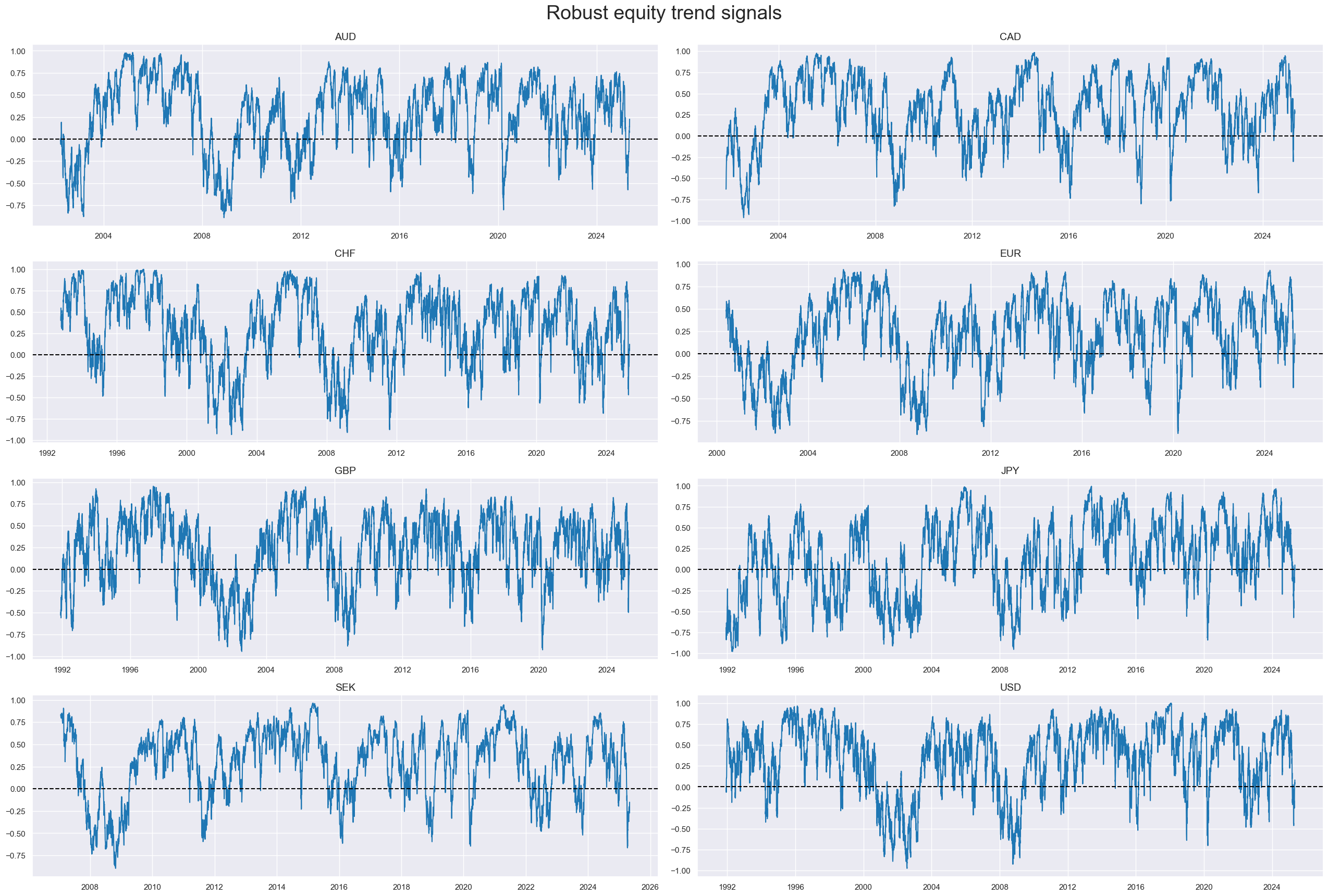
The timeline panel below shows robust trend signals for three countries with a long sample history (from 1992 for the U.S., Japan, and the UK) and five countries with a shorter history (from the 2000s). The sample length is determined by the availability of generic returns and the macro factors introduced further below. Robust trend signals are predominantly positive, which is not a surprise since they are based on excess returns (i.e. equity returns over funding costs) and equity exposure carries risk premia. They have been highly correlated across countries, with Pearson coefficients of 60-90%, and show both distinct cyclical swings and short-term volatility.
Macro support scores
Macro support factor here is a collective term for normalized macro headwind and tailwind factors. A positive support factor reinforces positive market price trend signals (tailwind) and opposes negative market trends (headwind).
We calculate a very simple composite macro support score based on up to four conceptual macro factor scores, each one representing an economic trend that, according to conventional theory, is supported by an equity returns trend and ends up opposing the latter. Each conceptual factor is calculated based on point-in-time macro-quantamental indicators of the J.P. Morgan Macrosynergy Quantamental System (JPMaQS) that represent the concept appropriately. However, no optimization has been applied, and it is likely that a broader macro support score, considering other signs of economic imbalances, would add more value.
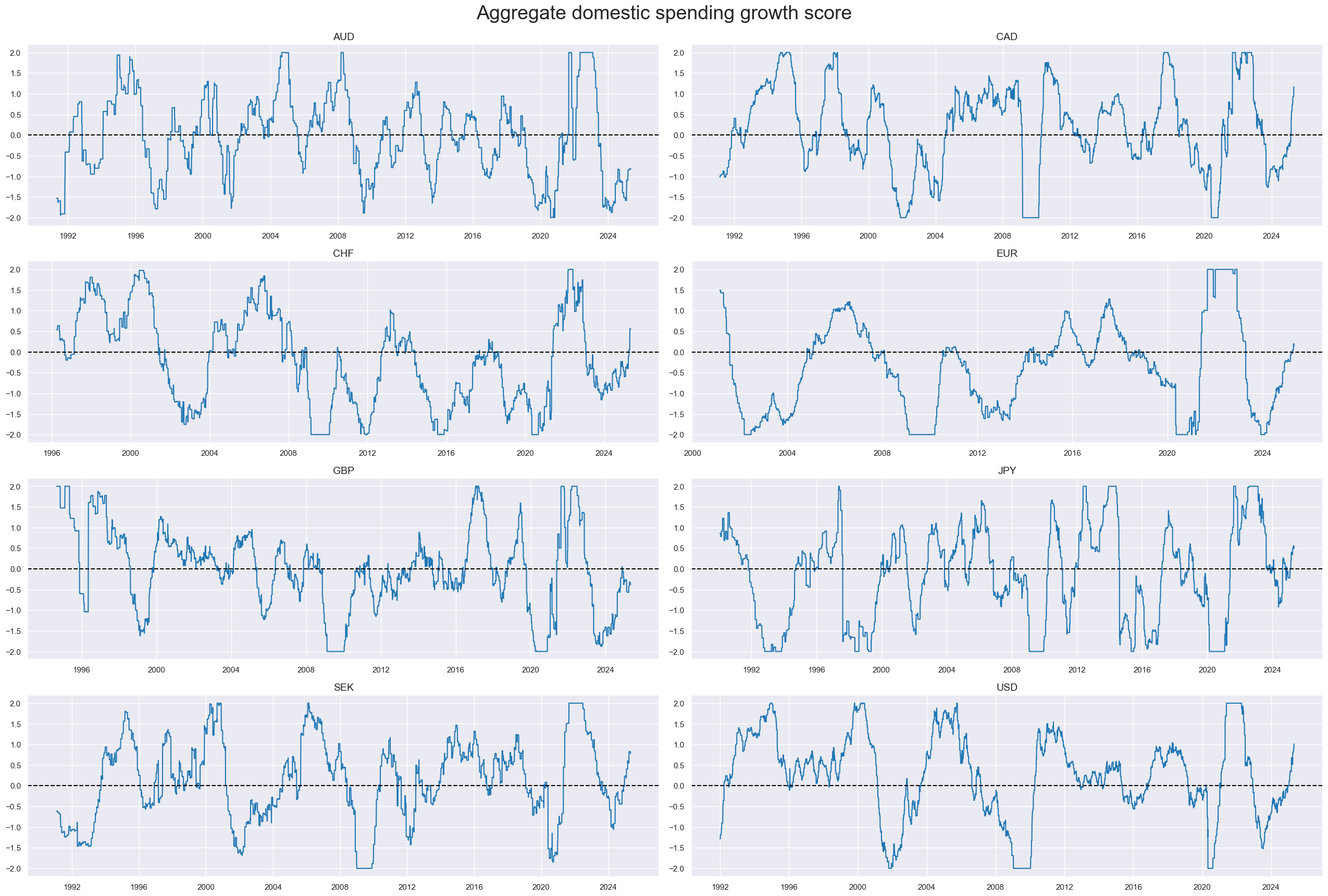
Conceptual factor 1: Excess domestic spending growth (negative for equity)
This factor seeks to measure the gap between aggregate final sales in the economy and long-term real or nominal GDP growth. It is an indicator of the state of the business cycle and future inflationary pressure and, all other things equal, calls for tighter monetary policy and rising real discount factors of future dividends.
The excess spending growth factor consists of three types of indicators
- Excess private consumption is the difference between the latest real private household consumption growth rate, as % over a year ago and the 3-month or quarterly average (documentation here) and the 5-year median of real GDP growth (documentation here).
- Excess retail sales growth is the average of (a) real sales growth as % over a year ago and 3-month average (view documentation) minus the 5-year median of real GDP growth, and (b) nominal sales growth (view documentation) minus the sum of 5-year real GDP growth and the effective inflation target of currency area (view documentation).
- Excess nominal import growth uses two growth rates of nominal merchandise import growth in local currency terms (documentation here) minus the sum of 5-year real GDP growth and the effective inflation target. The two growth rates are % over a year ago, 3-month average, and % 6 months over the previous 6 months, annualized and seasonally adjusted.
The indicators are normalized, then combined, with equal weight to the three types, and renormalized. Normalization in this post means sequential adjustment of values around their zero neutral level by using the point-in-time standard deviations and winsorizing values at a maximum of 2. Generally, in this post, the normalization of individual indicators uses both the cross-section and the panel standard deviations in equal weights. Re-normalization can be based on the panel alone. The panel below shows the resultant aggregate domestic spending scores. Across countries, they follow global cyclical patterns with the occasional mini-cycle.
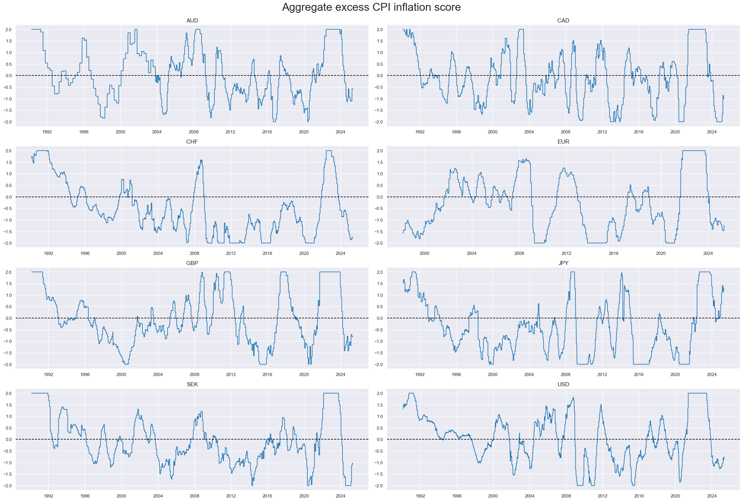
Conceptual factor 2: Excess CPI inflation (negative for equity)
This factor looks at the gap between various CPI inflation measures and the central bank’s effective inflation target. The effective inflation target is the estimated official inflation target plus an adjustment for past “target misses”. This adjustment is the last 3 years’ average gap between actual inflation and the estimated official target mean (documentation here). Above-target inflation biases monetary policy towards tightening and compromises a central bank’s ability to support markets in case of turmoil.
- Excess headline inflation is the difference between two CPI growth metrics and the effective target. The two growth rates are % over a year ago (documentation here) and % 6 months over the previous 6 months, annualized, seasonally and jump-adjusted (documentation here).
- Excess core inflation is the difference between two CPI growth metrics according to local convention and the effective target. The two growth rates are % over a year ago (documentation here) and % 6 months over the previous 6 months, annualized, seasonally and jump-adjusted (documentation here).
Similar to aggregate spending, aggregate excess inflation scores have come in multi-year cycles and shorter mini-cycles. They also displayed longer-term trends that could last a decade or more.
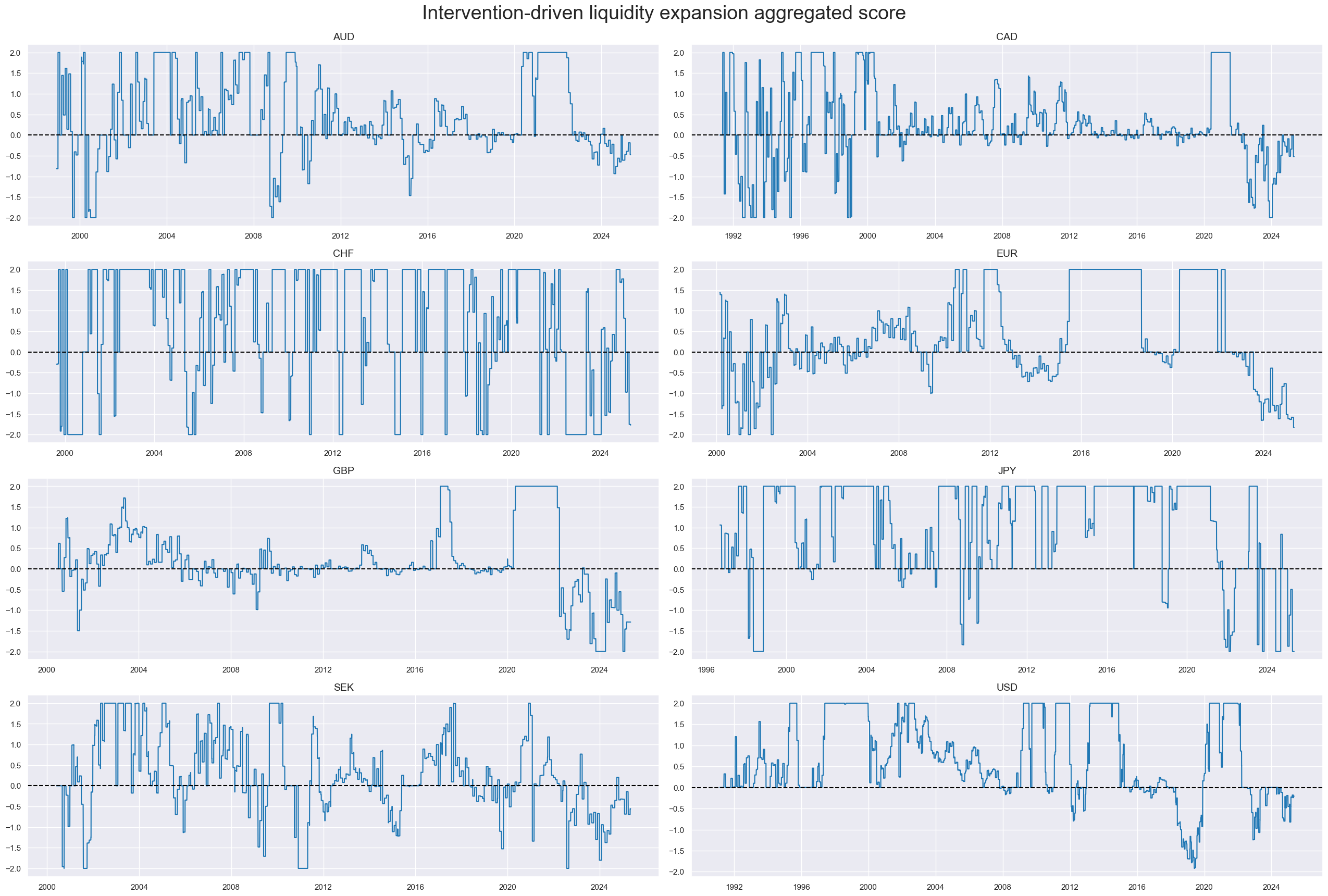
Conceptual factor 3: Intervention-driven liquidity expansion (positive for equity)
Intervention-driven liquidity expansion measures monetary base growth that is the consequence of central bank interventions. Two types of central bank interventions are considered: unsterilized FX interventions and domestic security purchases. The relation between intervention liquidity growth and subsequent equity returns should be positive, given that it is market-focused monetary easing.
Real-time estimates of intervention liquidity expansion are available on JPMaQS (documentation here). For this post, we look at Intervention-driven liquidity expansion as % of GDP. The highest average growth rates of intervention liquidity as % of GDP have been seen in countries that experienced more serious deflation risks over the sample period, such as Switzerland and Japan. Note that the sequential scoring increases the size of liquidity support scores in the 19990s and early 2000s relative to the time after the launch of global quantitative easing.
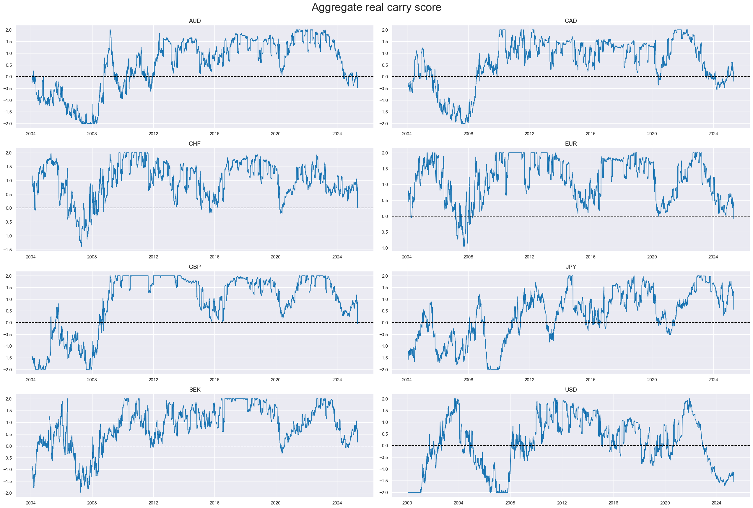
Conceptual factor 4: Excess real equity carry (positive for equity)
Generally, carry is defined as future return for unchanged market prices (Cross-asset carry: an introduction). Real carry accounts for the effect of expected inflation on contract value. For example, if a nominal asset price is unchanged, its real value is eroded by the rate of inflation. In the case of equity futures, which are funded positions, the estimated real carry on the main country index can be calculated as the difference between the average of expected forward dividends and earnings yield and the main local-currency real short-term interest rate. Higher carry means higher earnings and dividends relative to funding costs. Given that this trade-off is positively related to risk premia and monetary policy support, we expected positive explanatory power with respect to future returns.
Equity future carry metrics are available point-in-time on JPMaQS (documentation here). For this post, we look at simple carry, i.e., % annualised of notional of the contract, and vol-adjusted carry, i.e., % annualised of risk capital on position scaled to 10% (annualised) volatility target. Excess carry rates are set by subtracting the carry required for a carry-to-volatility ratio (“Carry Sharpe”) of 0.3. Normalization, averaging, and re-normalization follow the pattern of the other conceptual factors.
Index carry metrics are only available back to 2004, and, hence, they limit the sample periods that can use all three macro factors for backtesting. The aggregate real equity carry score has mostly been positive, particularly in the wake of financial crises. However, the score has also gone into deeply negative territory, particularly in times of economic downturns and financial turmoil.
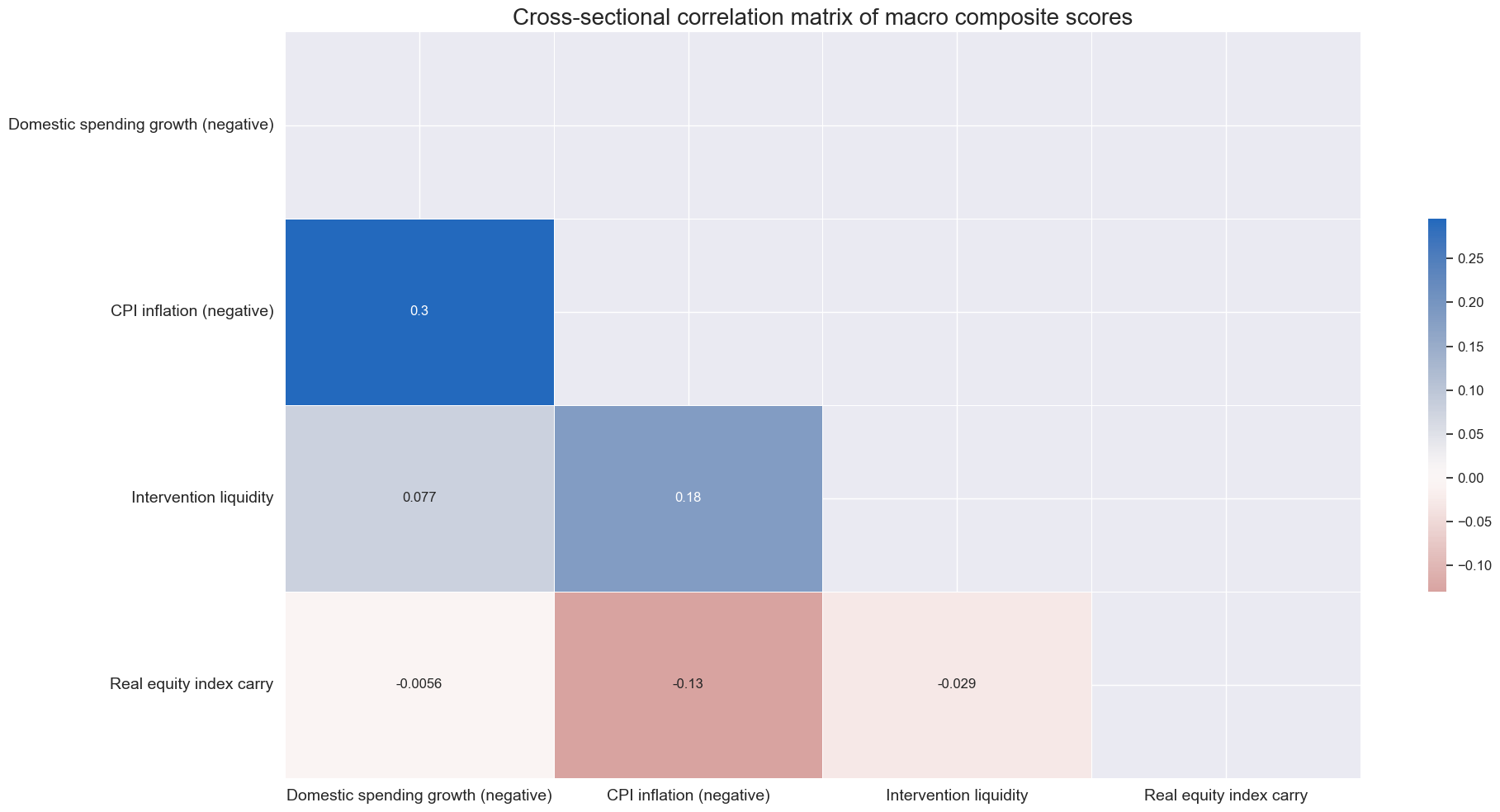
The non-carry macro factors have been positively correlated across the panel and based on monthly averages, albeit modestly so. This plausibly reflects that they are all subject to the state of the business cycle. Excess real carry has been uncorrelated with domestic spending and intervention liquidity and slightly positively with inflation, i.e., slightly negatively with the inflation support score.
Finally, we calculate aggregate macro support scores as averages of three macroeconomic factor scores and the real carry scores. This means all factor scores have been equally weighted, without selection and optimization, following the idea of “conceptual parity”.
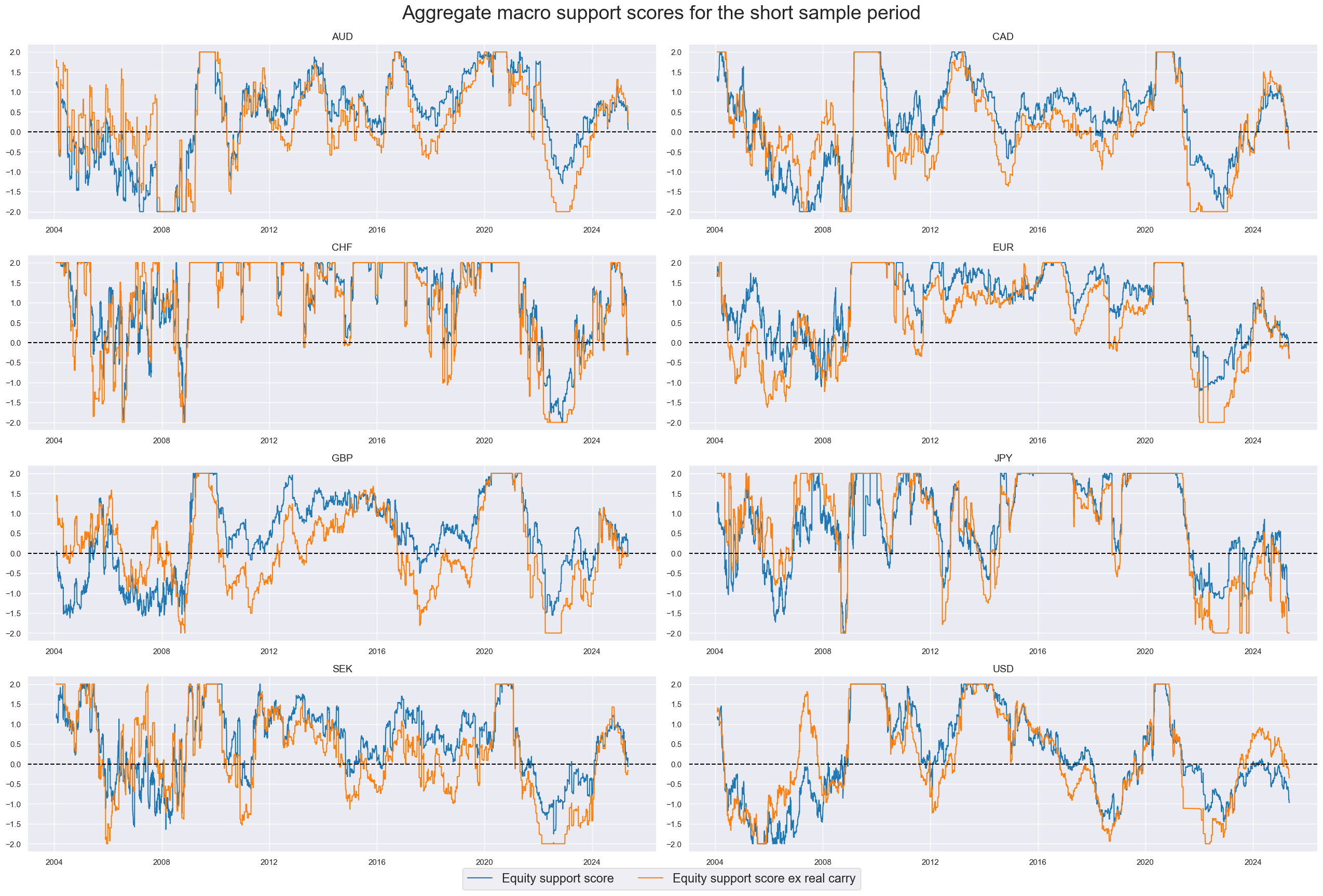
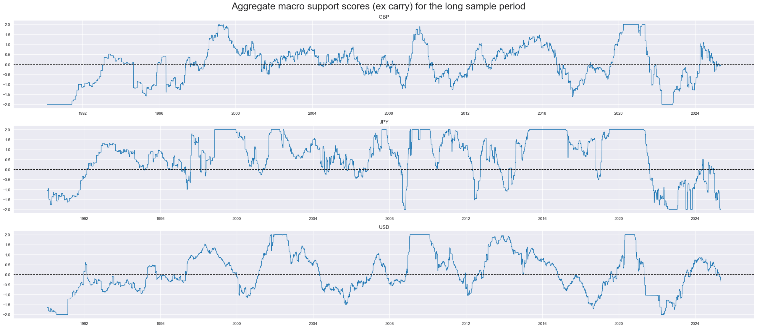
For subsequent empirical analysis, we use both a short sample period for all eight economies, from 2004 to 2025 (May) and a long sample for three of them, i.e. 1992-2025, for the United States, Japan, and the United Kingdom. This separation reflects data availability. Also, for the short sample, we calculate both a broad macro support score (that includes excess carry) and a narrow macro support score (excluding excess carry). For the long sample, excess carry cannot be considered. Generally, equity support scores have been slow-moving strategic factors that only flip signs at annual or lower average frequencies.
For the U.S., Japan, and the UK, aggregate macro supports cores of acceptable quality can be calculated back to 1992. However, the range of available high-quality quantamental indicators is narrower, and some indicators, such as point-in-time inflation targets, had to be approximated very roughly. This means that the quality of the macro support scores, in terms of representing actual information states, is a bit lower for the 1990s than for the subsequent decades.
Modified and balanced robust trends
Next, we adjust the robust trend signals for all eight countries for the state of local macro support. This means we reinforce a market trend signal that coincides with macro tailwinds and reduce or even flip a trend signal that coincides with macro headwinds. For illustration, we use two simple methods for adjustment: modification and balancing.
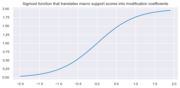
Modification means that we adjust the trend signal strength but never flip its sign. Specifically, here we multiply the original trend signal with a coefficient that can take values between 0 and 2. It can double the original trend signal or reduce it to zero, depending on the agreement of the macro situation with the price trend. The modification coefficient is a logistic (sigmoid) function of the macro support z-score.
Specifically, the adjustment implements the following equation:
modified_trend = ((1 – sign(trend)) + sign(trend) * coef) * trend
for
coef = 2/(1 + exp(-2 * macrosupport_score))
where trend means the original robust trend score, sign() returns the sign of its element as 1/-1, and macrosupport_score denotes the composite macro support score.
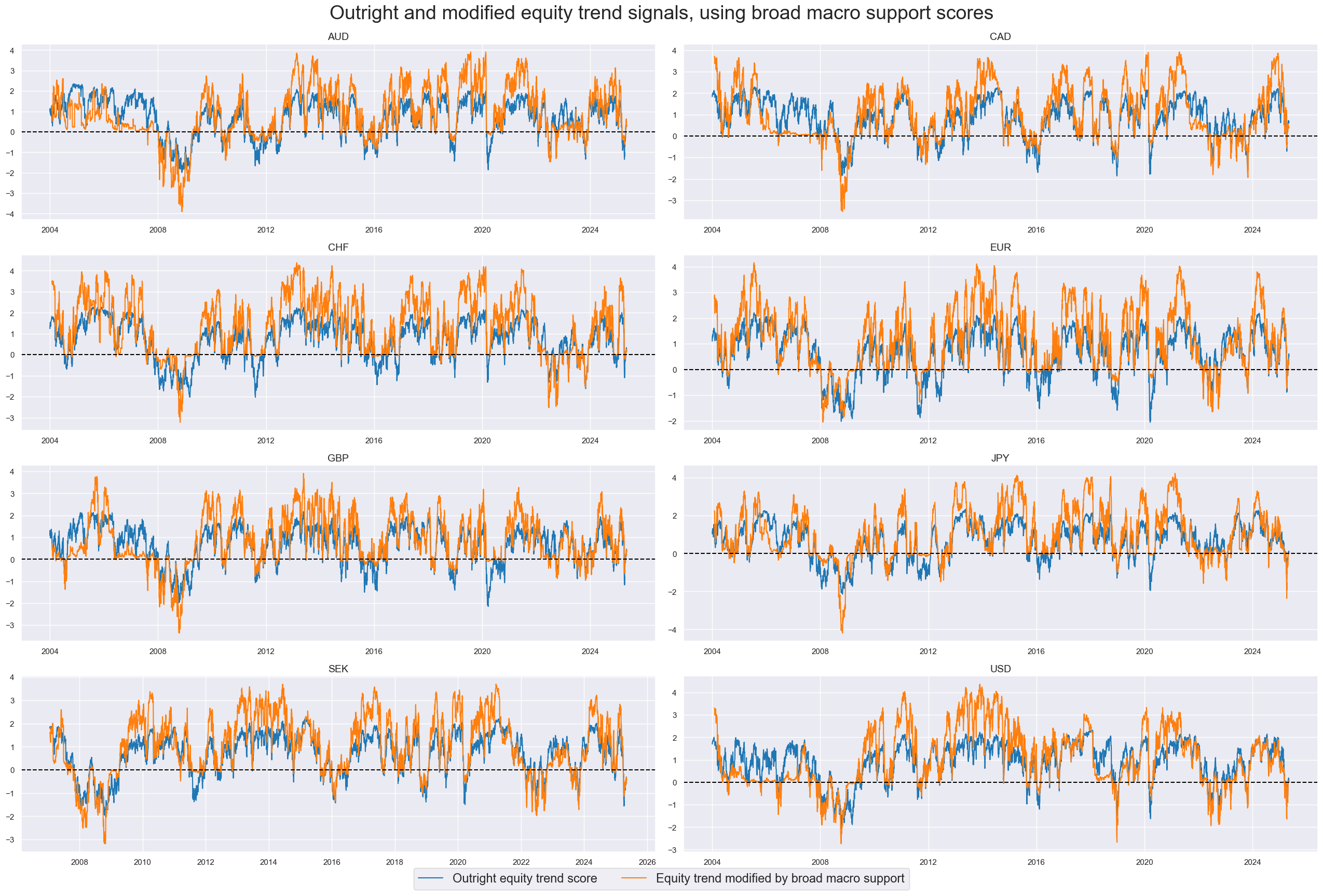
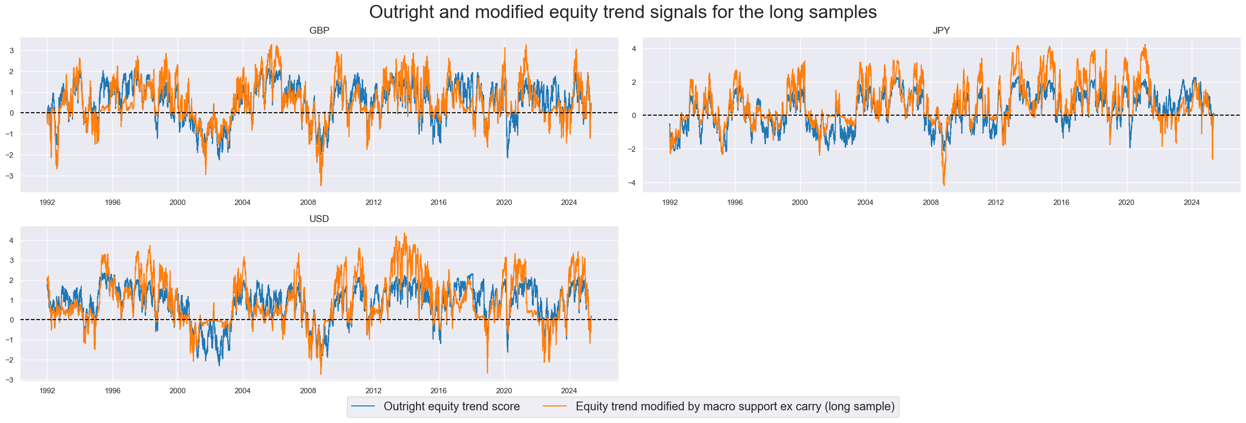
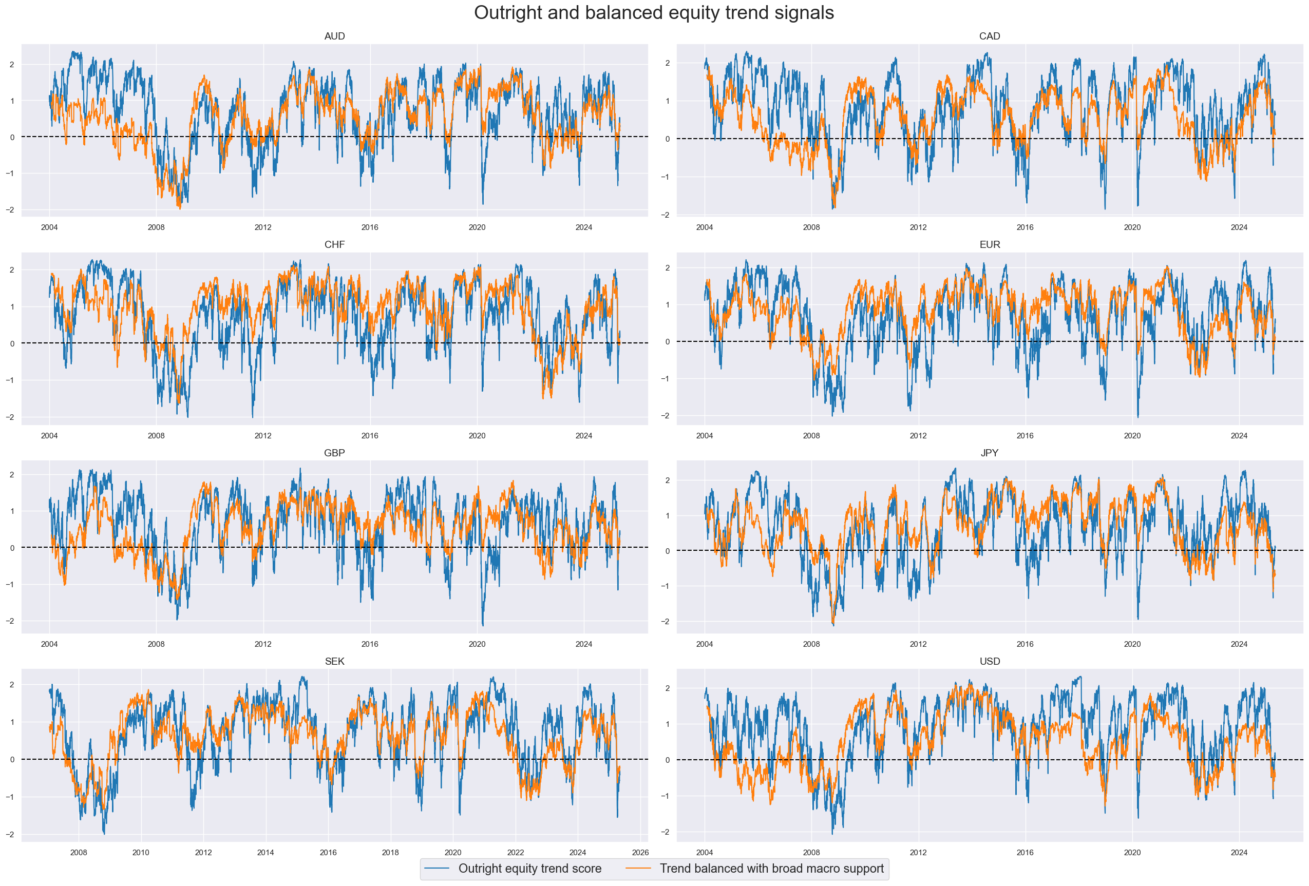
The panel below shows the original trend scores and their modified values for the short samples, using the local broad macro support scores. Modification dampens or enhances signals depending on the economic state and visibly so. Thereby, the pattern of the trend signal changes visibly across all countries, even though it never changes the sign.
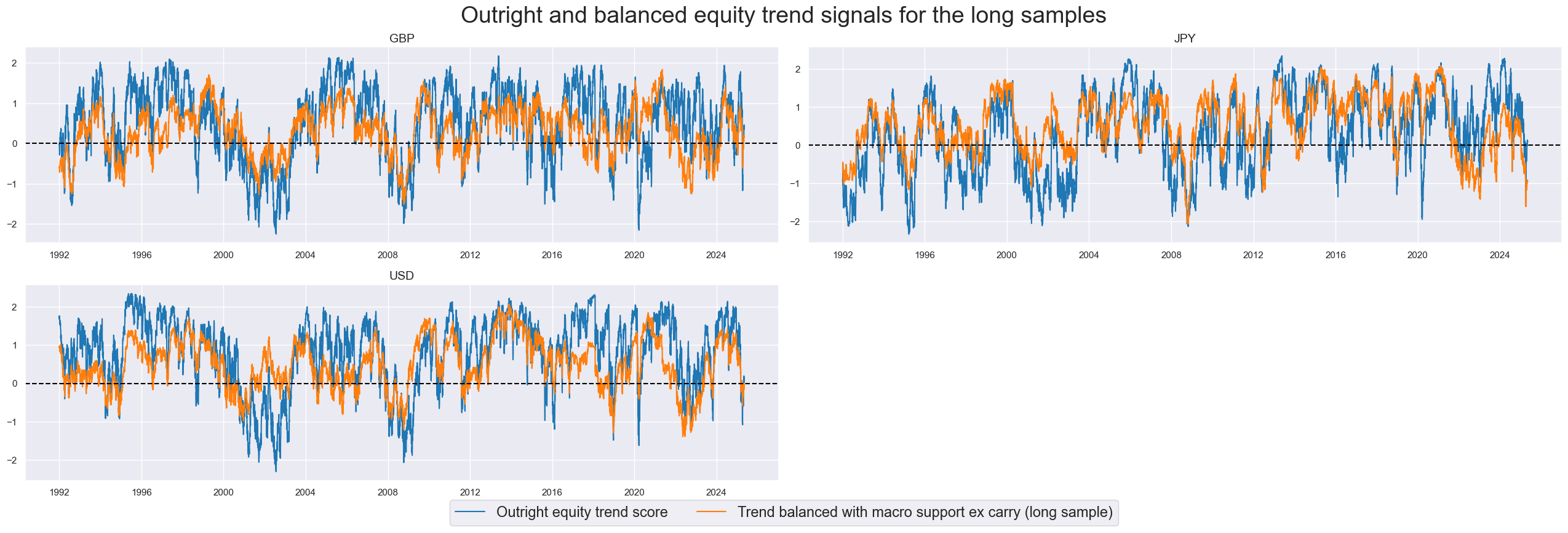
The charts below show the original robust trend scores and their modified values for the long sample. These only use support scores without carry, as the data for that latter would only begin in 2004. Differences are visible and particularly large for the U.S and the UK.
The alternative to trend modification is balancing. Balancing here means that we simply take the average of the robust trend score and the macro support score. Balanced trend signals can have different signs than the original trend score if the macro support constitutes a strong enough headwind to the market trend. Balancing causes greater even differences between original and adjusted signals than modification and interferes more with the basic characteristics of simple robust trend following.
Evidence of the value of robust trends
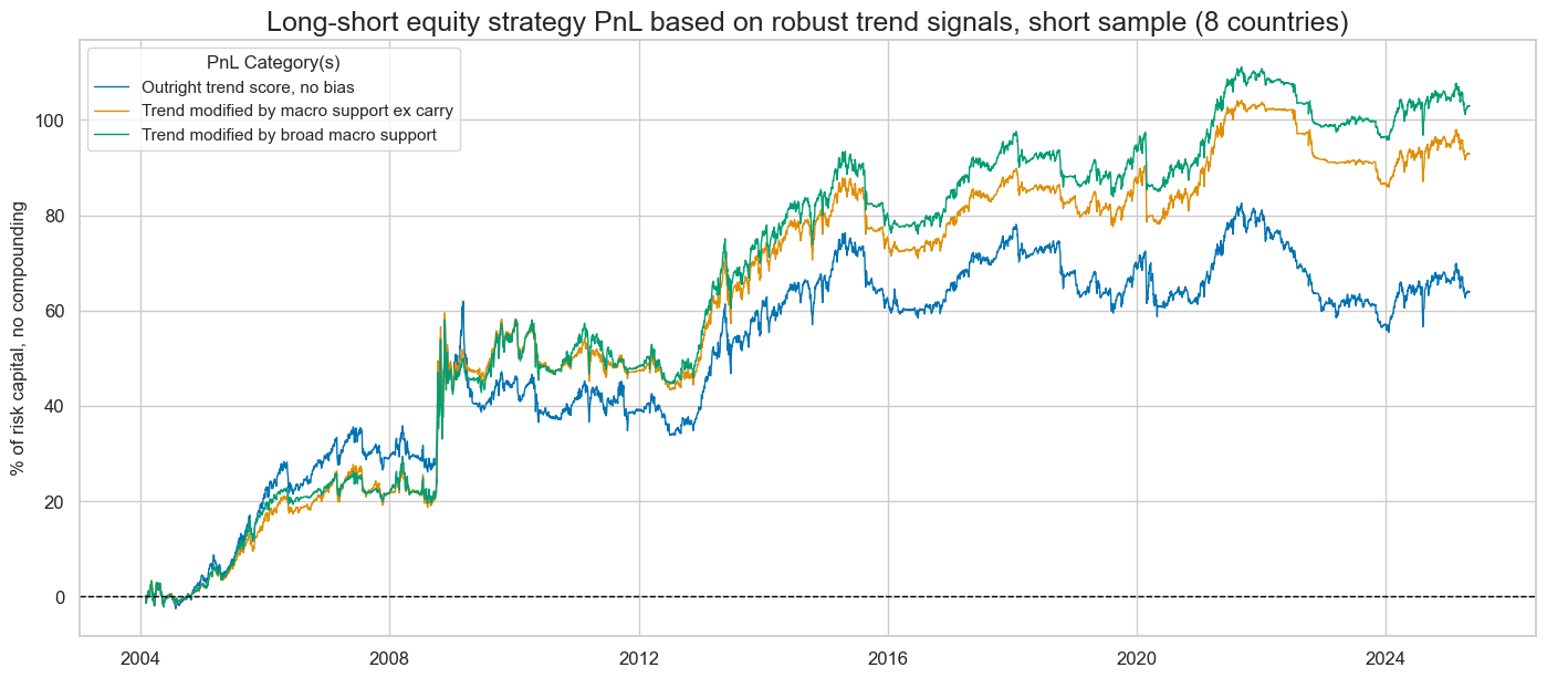
We evaluate the economic value of outright and adjusted robust equity trend scores by means of naïve PnLs, using standard rules of Macrosynergy strategy research. This means that long and short positions are set based on outright or adjusted trend scores across the eight or three developed equity market index futures. Positions are rebalanced monthly based on signals available at the end of each month, considering a one-day slippage added for trading, leading to two positions on the second trading day of the month. This simplistic rebalancing is a standard for testing the economic value of factors and is not optimal. Transaction costs are disregarded as they depend heavily on transaction size. The only risk management consideration is the capping and flooring of signals at two standard deviations to limit risk concentration. The long-term volatility of the PnL for positions across all currency areas has been set to 10% annualised. This is no volatility targeting but merely a convention that facilitates the comparison of risk-adjusted returns in charts.
For the short sample 2004-2025, all trend following strategies have rendered a positive risk-adjusted return without much correlation to the S&P 500. Modified trend scores outperformed the outright robust trend signal, particularly from the 2010s onward. Sharpe ratios have generally been low, at 0.3 for outright market trend scores and 0.4-0.5 for modified trends. Sortino ratios have been 0.4 for the market trend and 0.6-0.7 for its modified cousins. Low risk-adjusted returns are plausible, given that we are looking at a single-principle strategy and little diversification of signals and returns (equity markets are highly correlated). Also, we made no attempt at signal optimisation. However, the robust and modified robust trend strategies of this type can be operated with very high volumes in liquid markets and are complementary to long-only exposure and to cross-sector equity strategies (view posts here and here) and cross-sector equity strategies (view posts here and here).
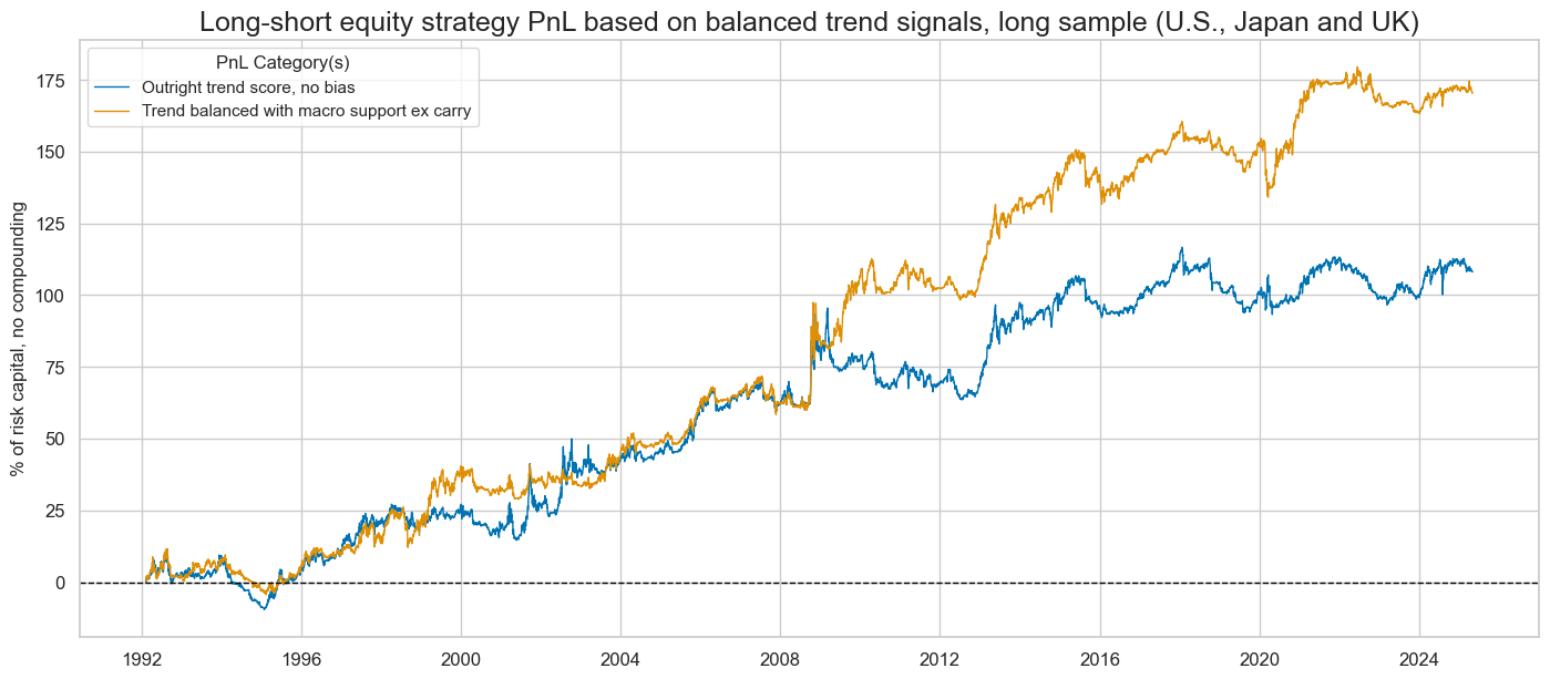
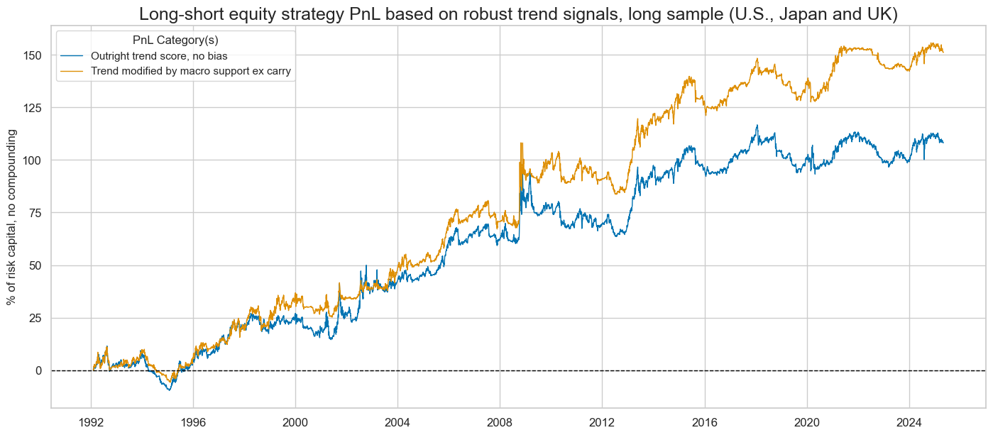
Long-term positive risk-adjusted value generation of robust outright and macro-modified market trend signals has been confirmed for the long sample of just three countries since 1992. Again, the risk-adjusted returns of the naïve PnL have been modest with Sharpe ratios of 0.3-0.5 and Sortinos around 0.6. Trend modification by macro support scores has consistently enhanced value, in particular from 2008 onward. Correlation with the S&P 500 has been near zero.
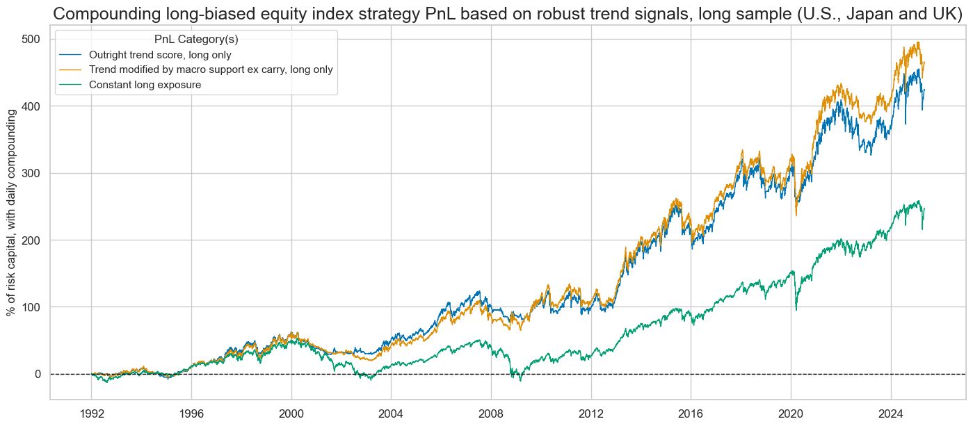
The benefits of robust modified trend signals become more obvious when viewed in conjunction with a long-only strategy and the consequences of compounding returns. The below chart shows the effects of modifying a constant long-only strategy by the long-short signals, such that exposure is either doubled or reduced to zero, depending on the strength of the modified trend scores. Moreover, risk capital is increased or reduced by returns, similar to a cash portfolio. Equity portfolios managed by the modified robust trend scores since 1992 would have produced almost double the return of a simple long-only strategy.
Results are similar for naïve long-short PnLs based on balanced signals. For the short sample, the balanced trend signals have yielded positive PnL with little broad equity market correlation. However, the outperformance of the macro-enhanced signals has been greater through balancing, with Sharpe ratios of 0.6-0.7 versus 0.3 without consideration of macro support. Sortino ratios of the balanced trend signals have been as high as 0.8-0.9. Outperformance has been concentrated on periods of pronounced economic cyclical momentum, such as during the great financial crisis and the COVID-19 pandemic.

The macro enhancement has added consistent value to outright robust trend following for the 3-country long sample since 1992. The outperformance became particularly pronounced over the past two decades, possibly reflecting the limited availability of quantamental sub-indicators in the 1990s compared to subsequent decades. Also, some important structural indicators, such as effective inflation targets, have not been available for that period and needed to be approximated, as explained above.