Surprises in industry and construction activity are plausible predictors of short-term future returns for commodities that are heavily used in these sectors. This hypothesis can be evaluated using quantamental economic surprises, which are point-in-time differences between estimated market expectations and actual reported values of economic indicators, measured at a daily frequency.
We specifically assess the predictive power and economic value of global surprises in survey and production indicators across 32 economies. Country-level surprises are first standardised and then aggregated into global composites, weighted by each economy’s share in global industry. Since 2000, the resulting global surprise indicator has been a statistically significant predictor of returns for an industrial commodity futures basket. A simple daily trading strategy based solely on this signal would have generated material risk-adjusted returns with little correlation to global equity markets. Further hedging against non-growth-related factors, such as monetary risk proxies, can improve performance.
The post below is based on Macrosynergy’s proprietary research. Please quote as “de la Porte Simonsen, Lasse and Yavari, Cyrus, ‘Economic surprises and commodity futures returns,’ Macrosynergy research post, June 2025.”
A Jupyter notebook for auditing and replicating the research results can be downloaded here. The notebook operation requires access to J.P. Morgan DataQuery to download data from JPMaQS. Everyone with DataQuery access can download data except for the latest months. Moreover, J.P. Morgan offers free trials on the complete dataset for institutional clients. An academic support program sponsors data sets for research projects.
The basics of quantamental economic surprises
Quantamental economic surprises are defined as point-in-time deviations of economic indicators from reasonable market expectations. Market expectations are estimated by practical econometric models, rather than economist surveys. Both expectations and surprises are calculated based on sequences of the underlying time series, also called “vintages”. For example, expectations and surprises to production growth for any given day are calculated based on the production index vintages of the previous day and the same day, respectively. Generally, vintage updates trigger two types of surprises:
- First-print events are differences between a macroeconomic indicator on a release date and its expected value. A release date is the day on which any underlying economic time series adds a new observation period. Expected values are model estimates using the latest vintages prior to the release date.
- Pure revision events are changes in an economic indicator on non-release dates. They are revisions of previously released observation periods. By default, quantamental surprises assume that all revisions are surprises, i.e., that preliminary vintages are the best predictors of final vintages.
A quantamental indicator of economic surprises records the values of these two events on their publication dates. It records zero values for all other days. The key benefit of surprises created by this methodology, versus those based on surveys, is that they follow common standards and are available for a wide range of indicators, not just the ones surveyed in release calendars. Also, quantamental economic surprises include all changes in economic history, not just scheduled releases. Thereby, quantamental surprises are a more complete and internationally comparable data set than survey-based surprises. For a full explanation of quantamental economic surprises, view a previous post, Quantamental economic surprise indicators: a primer.
Industrial commodity futures and the theoretical impact of economic surprises
This post examines the predictive power of quantamental economic surprises in global industry and construction on industrial commodity prices. We define the tradable universe of industry-related commodity futures as a set of twelve USD-denominated front futures of three categories:
- Base metals contracts are LME aluminium (ALM), Comex copper (CPR), LME Lead (LED), LME Nickel (NIC), LME Tin (TIN), and LME Zinc (ZNC).
- Precious metals contracts with industrial use are NYMEX palladium (PAL) and NYMEX platinum (PLT).
- Crude and fuels contracts here include ICE Brent crude (BRT), NYMEX WTI light crude (WTI), NYMEX RBOB Gasoline (GSO), and NYMEX Heating oil (HOL).
All the above commodities are used to some significant degree in industry and construction. This means that revisions of output and demand in these sectors should affect demand for the 12 commodities. Hence, by themselves, positive economic surprises in industry and construction should trigger positive short-term returns in all related futures positions. The focus of the empirical analysis in this note is on returns on volatility-targeted positions to make risk exposure comparable across commodities and periods in time. This means that all positions are scaled to a 10% volatility target based on the historic standard deviation for an exponential moving average with a half-life of 11 days. Positions are rebalanced at the end of each month.
Cumulative returns on volatility-targeted futures positions have been positive in the long run for all industrial commodities, pointing to risk premia for long positions. Patterns and extent of passive returns have been quite different, however, reflecting many powerful forces that are not accounted for by economic surprises, such as supply shocks and structural demand shifts.
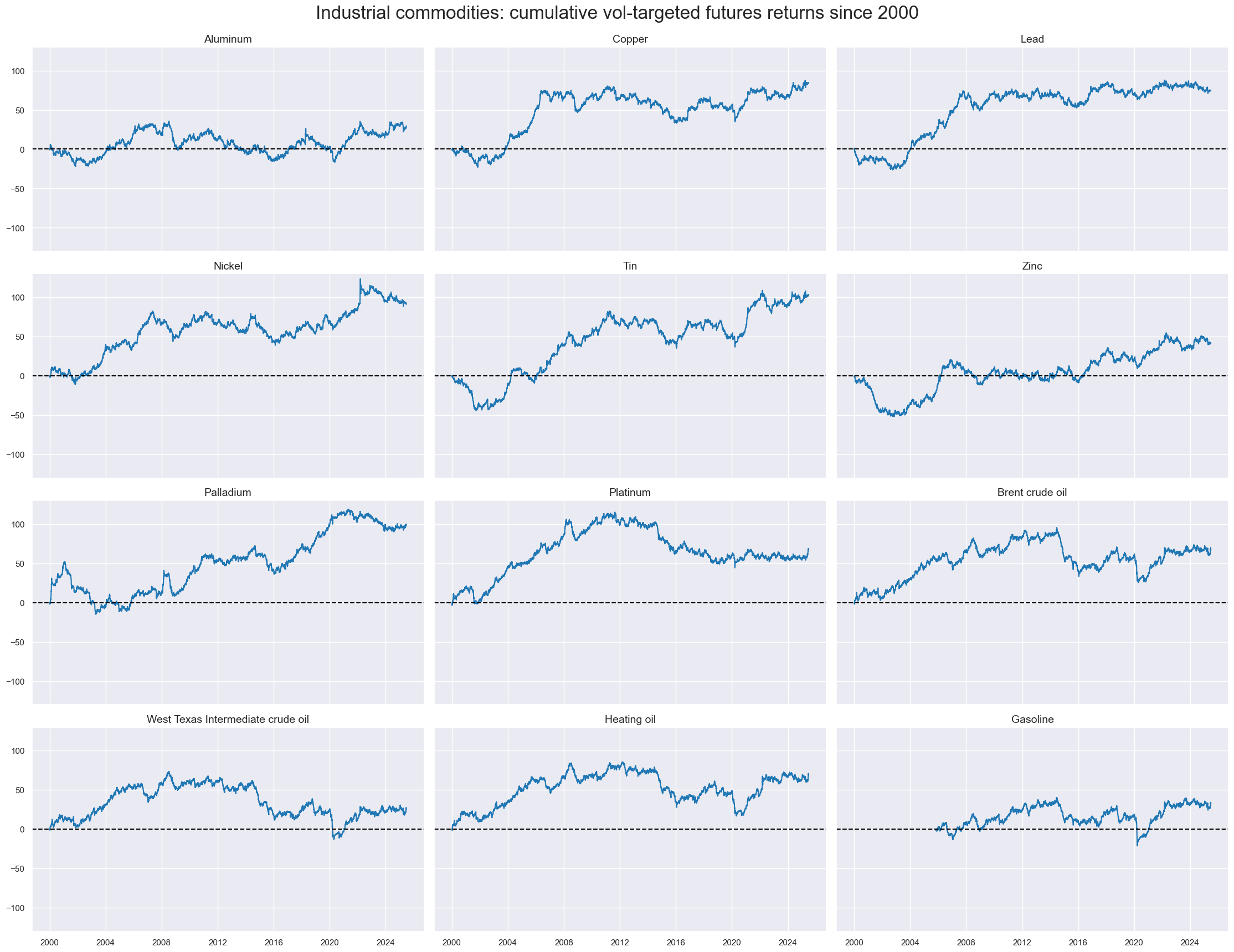
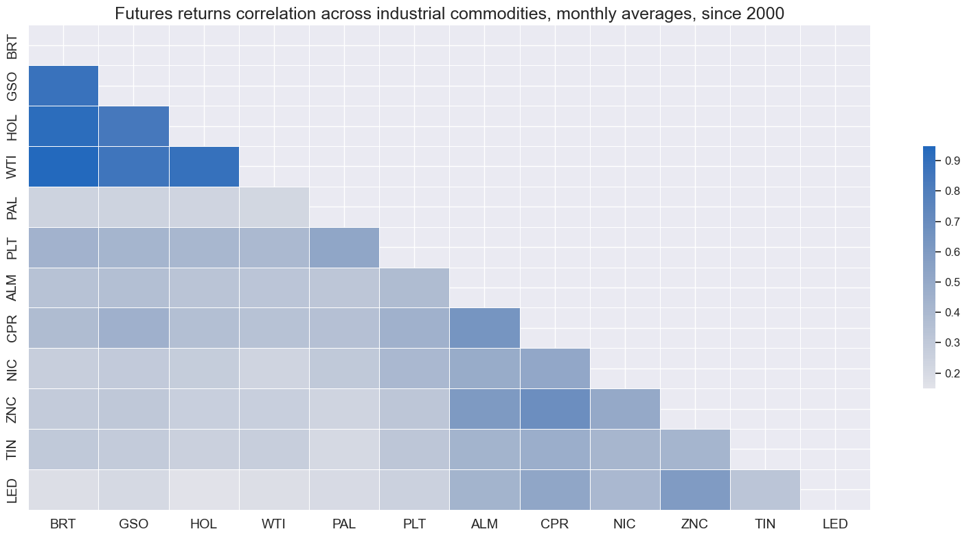
Also, all pairs of industry-related commodity futures returns have been positively correlated at a monthly frequency, with correlation coefficients ranging between 10% and 90%. Cross-correlation has been particularly high within the crude and fuels group and, to a lesser extent, within the base metals group.
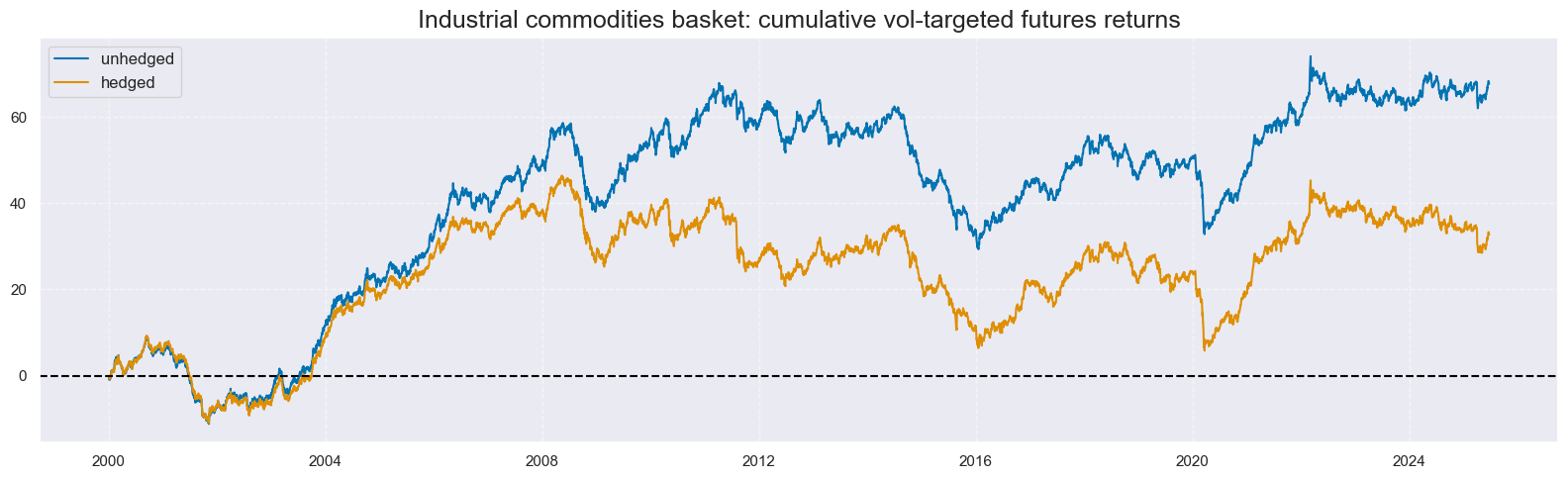
For the empirical analysis in this post, we focus on the returns of a risk-parity basket of all twelve commodities, whereby individual contract positions are all volatility-targeted. This is approximately equal to the average volatility-targeted return across the contracts. As shown in the empirical sections further below, we can examine the return of an outright risk-parity basket and that of a basket that has been partially hedged against factors other than demand shocks.
The stages of calculating global economic surprises
Our main hypothesis is that economic surprises to global industry and construction predict short-term industrial commodity basket returns. Daily time series of surprises for the most important economies can be downloaded in point-in-time format for a wide range of countries from the J.P. Morgan Macrosynergy Quantamental System (“JPMaQS”).
For first print events, the benchmark expectations for any indicator are the value that one would predict by forecasting the underlying time series levels with an autoregressive moving average model of first order, called ARMA(1, 1). By default, this model accounts for the correlation of seasonally-adjusted index changes, the effects of past errors, and “base effects”, i.e., biases that result for extraordinary increases or declines in the base period of a growth rate. We look at surprises in up to 32 developed and emerging market economies, which are enumerated in Annex 1 below, for three types of indicators.
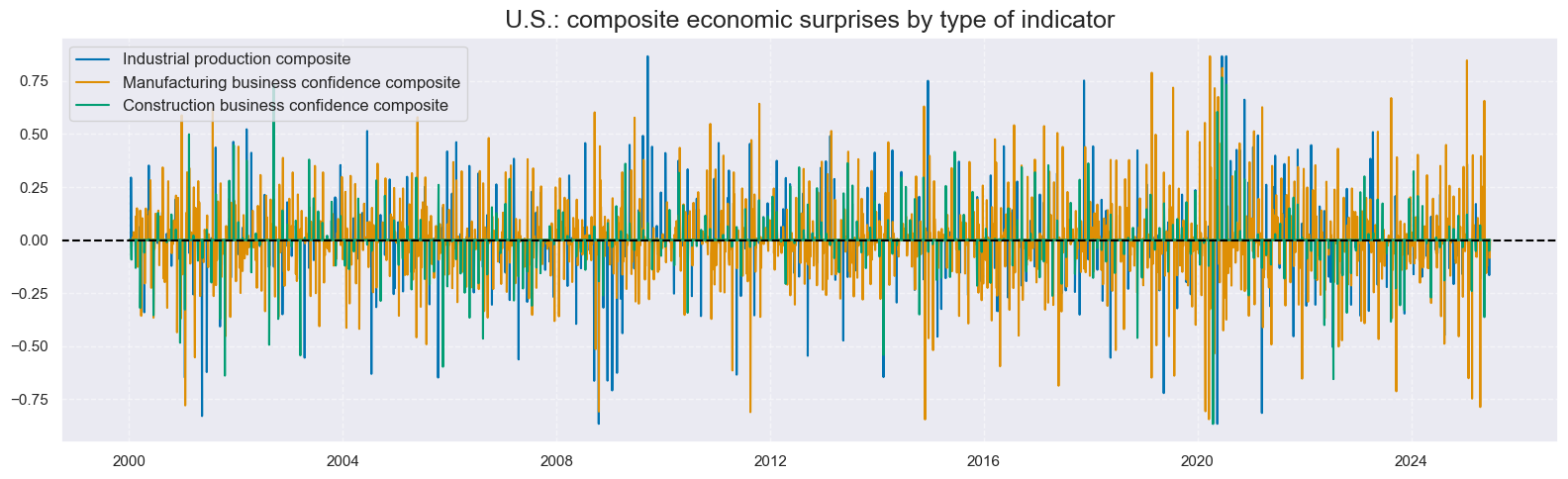
- Industrial production surprises are calculated for three growth rates, [1] % over a year ago as 3-month moving average, [2] % 6 months over the previous 6 months, seasonally adjusted and annualised, and [3] % 3 months over the previous 3 months, seasonally adjusted and annualised (documentation here).
- Manufacturing business confidence surprises are calculated for the seasonally adjusted level of local manufacturing confidence scores, for the 3-month moving average of that level, as well as for four rates of change: the difference of the last 3 months over the previous 3 months, the difference of the last 6 months over the previous 6 months, the difference of a year ago, and the difference over a year ago in 3-month moving average (documentation here).
- Construction business confidence surprises are calculated for the same transformations as for manufacturing confidence (documentation here).
We limit the analysis here to surprises from 2000, as older data on JPMaQS are often based on proxy vintages for many countries and lack the same quality as those from the past two and a half decades. To generate trading signals for a single commodity futures basket, we need a single time series of global economic surprises. This involves seven preparatory steps.
Step 1: Normalisation of surprises across indicators
For each indicator, daily surprises are divided by the standard deviation of the surprises on release dates with new observation periods. The standard deviations themselves are estimated point-in-time based on the previously available history of first-print surprises, applying an exponential moving average with a half-life of 36 release dates.
Step 2: Winsorization of normalised surprises
All normalised surprises are capped and floored at three standard deviations on the negative and positive side to mitigate the influence of large outliers.
Step 3: Annualization of surprises across frequencies of underlying data series
Longer observation periods provide more information on economic changes than shorter ones. For example, a quarterly CPI report reveals a larger price development than monthly CPI data, as more time has passed. To equalise the information value of indicators across different frequencies, we divide each by the square root of its implied number of observation periods in the year.
Step 4: Aggregate surprises across transformations of an indicator
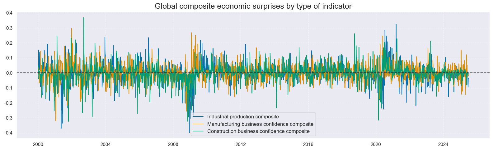
Until this point, surprises have been computed and standardised separately for each transformation of the three core indicators: industrial production, manufacturing confidence, and construction confidence. The use of multiple transformations is justified, as market participants rely on varying conventions, and different lookback periods may capture distinct aspects of vintage updates. However, once surprises are normalised and annualised, they can be averaged to form a single composite surprise series per base indicator. This process—referred to as conceptual aggregation—yields three composite surprise series for each economy.
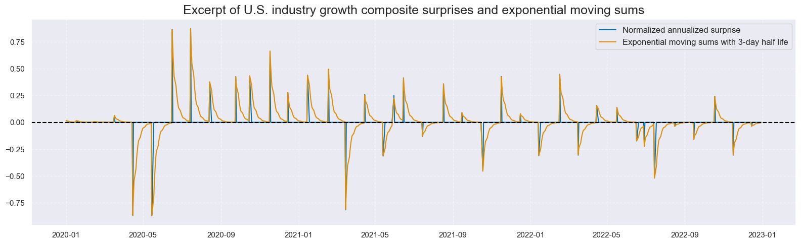
Step 5: Exponential moving sum of aggregate surprises
We assume that the impact of economic surprises on broad market perceptions unfolds over several days but largely dissipates within a week. Accordingly, the analysis below focuses on exponential moving sums of composite surprises with a half-life of three days. This specification implies that approximately 95% of a surprise’s informational value fades within the span of a standard workweek.
Step 6: Global aggregation of composite surprises across economies
For predicting global commodity returns, we form weighted global averages of daily exponentially-averaged economic surprises. The basis of weights is point-in-time industrial value-added in USD for the 32 economies (documentation here). The aggregation results in three global surprise indicators, each of which effectively communicates surprises every day.
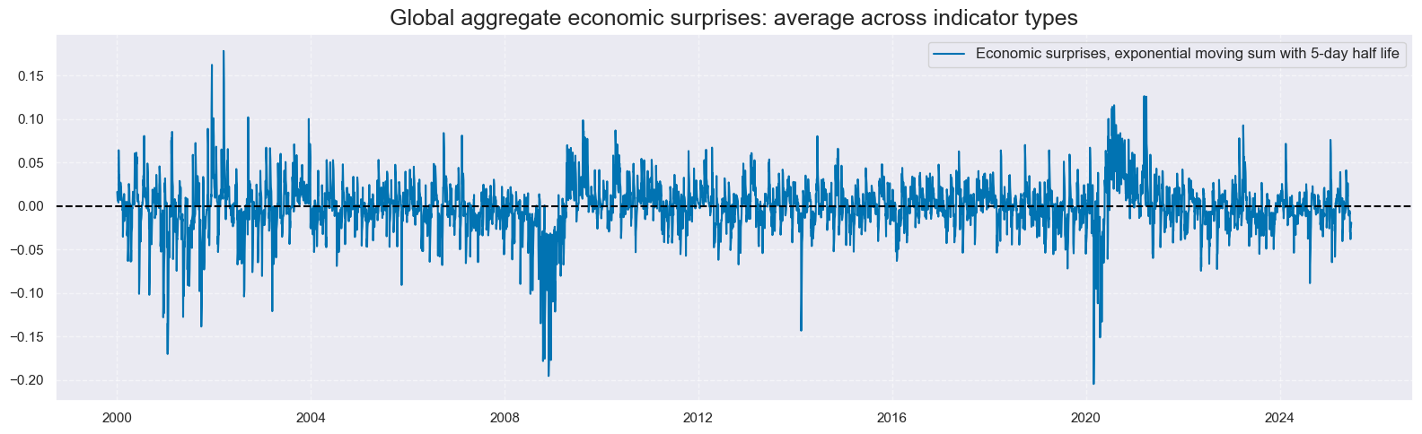
Step 7: Global composite aggregation across types of indicators
Finally, we also calculate a single global economic surprise aggregate as an unweighted average of the composite surprises of the three types of indicators. Note that if one type of indicator has a shorter history than others, then the average is formed based on the available ones.
Predictive power and economic value
We evaluate the single global economic surprise series as a daily signal for trading a risk-parity-weighted industrial commodity futures basket. For proof of concept, the strategy employs no optimisation or diversification. This simplicity is not intended to suggest that equal-weighted signals or positions are optimal; rather, it serves to enhance transparency and credibility in the assessment.
We assume that commodity basket positions are updated at the end of each trading day in accordance with the economic surprise signal for that day. Since surprises are short-term signals, we cannot allow for a full day’s slippage for trading, as we do for non-surprise quantamental indicators. Fortunately, global economic surprises, including those of the U.S. time zone, are broadly available before the futures markets close in Europe. We trade a single commodity basket position based on a single global economic surprise-based signal. The assumption is that at the end of each day, a position is taken based solely on the economic surprise signal.
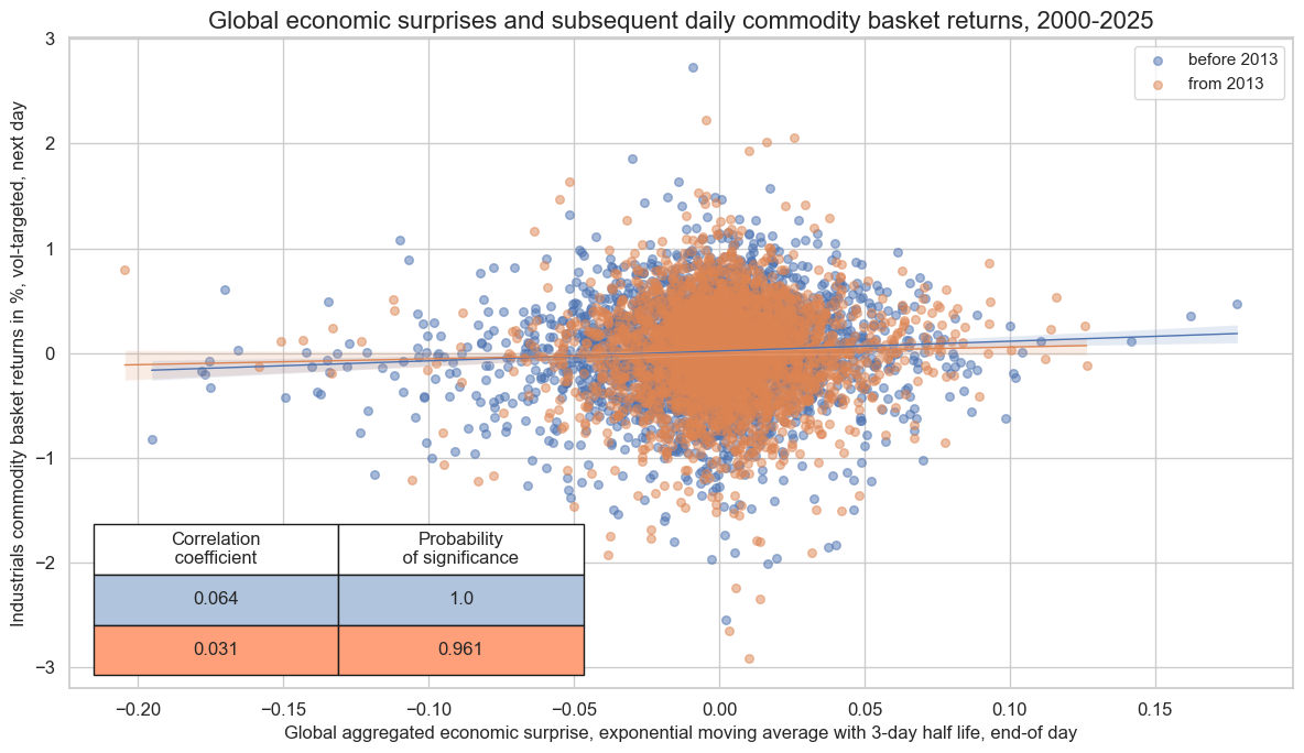
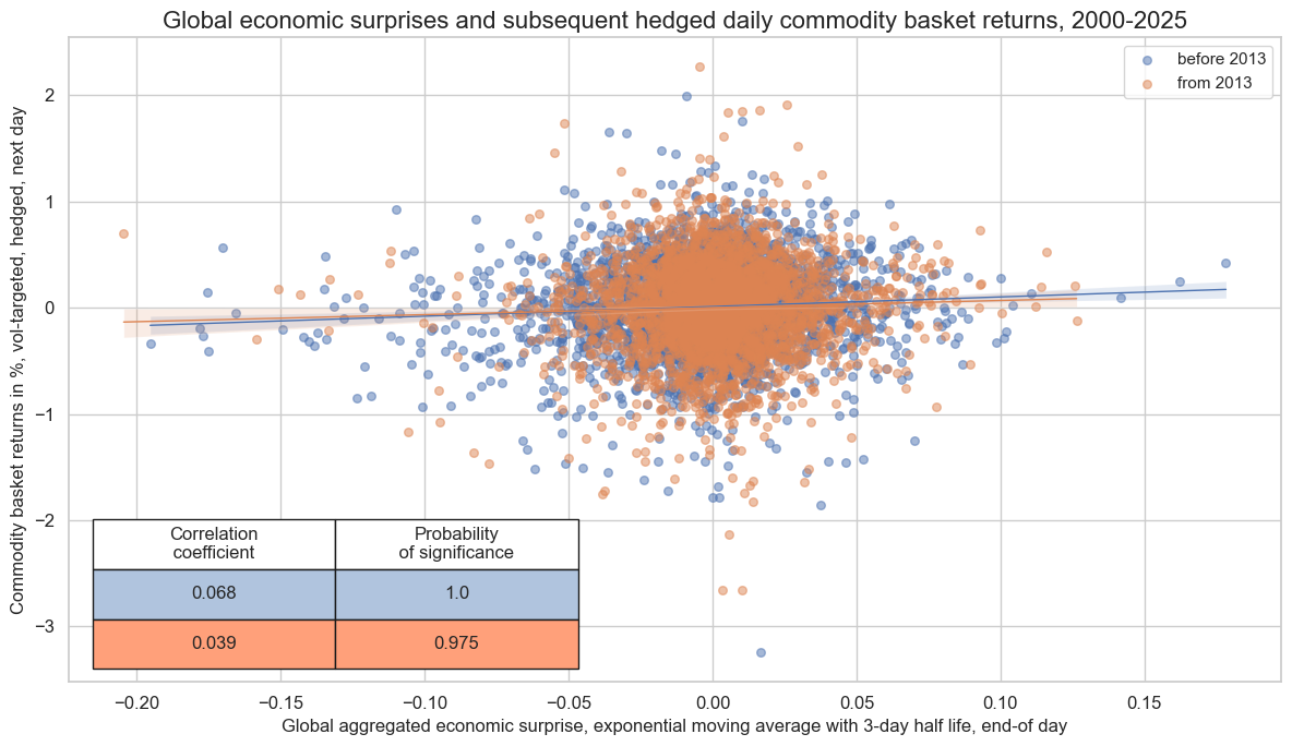
The regression scatter plot below shows the relationship between end-of-day global economic surprises and next-day commodity futures basket returns for the period from 2000 to 2025 (as of June). The relationship has been positive and highly significant. The probability of significance has been near 100% for the full sample, and above 95% for the two halves of the sample timeline.
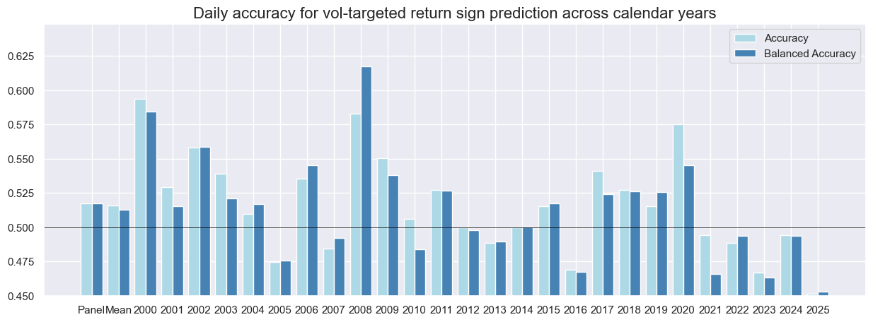
The chart below shows the accuracy (ratio of correctly predicted signs of returns of the next day) and balanced accuracy (average ratio of correctly predicted positive and negative signs) for the full sample and all full calendar years. Daily accuracy since 2000 has been 51.7%, which counts as a weak statistical signal in general, but a decent one for a simplistic macro trading strategy. Generally, accuracy has been higher in times of pronounced cyclical economic swings and lower in more “normal periods”. This suggests that economic surprise-based trading may be complementary to risk premium strategies that work better in “normal” times.
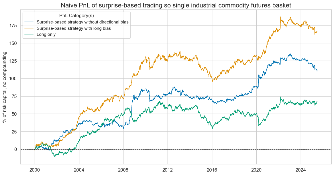
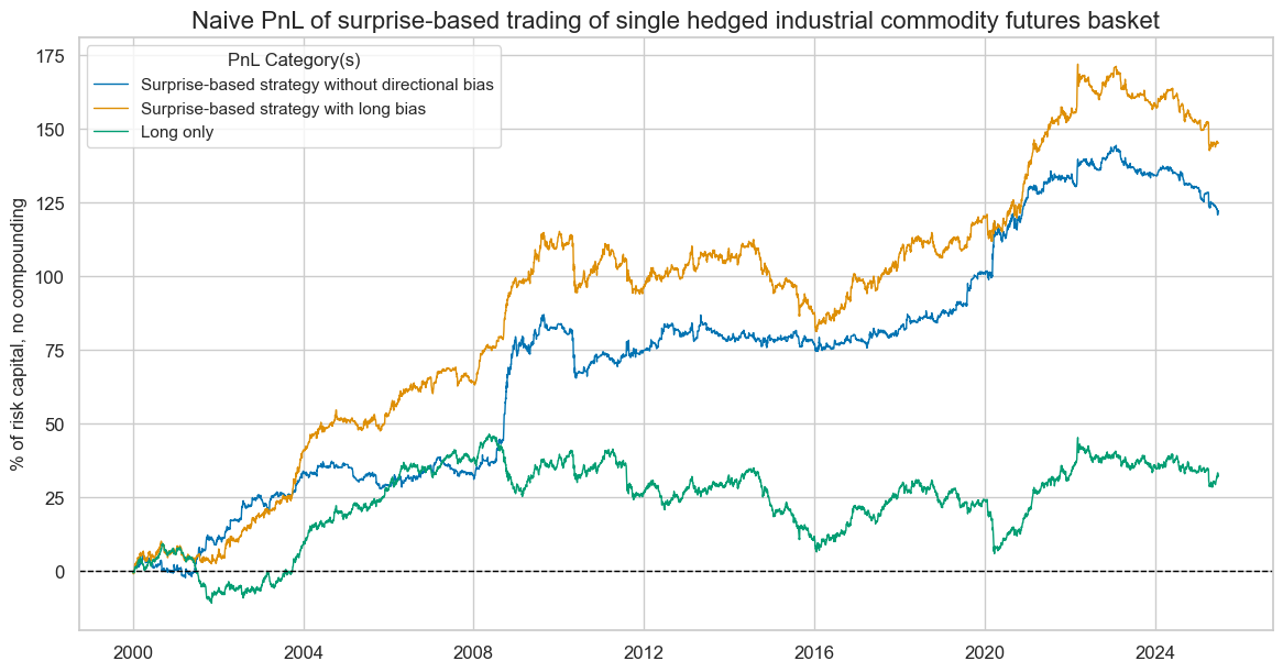
We assess the economic value of a primitive strategy that simply takes a position at the end of each day in proportion to a normalised global economic surprise indicator of that day, up to a maximum of two standard deviations. The naïve PnL does not consider transaction costs or compounding. Furthermore, we calculate two strategy versions, one without directional bias and one with a long bias (by adding one standard deviation to the signal). The latter serves as a comparison with a long-only risk parity portfolio of the twelve futures contracts.
Naïve PnL analysis shows material long-term economic value, but also great seasonality. The naïve PnL of the unbiased surprise strategy achieved a long-term Sharpe ratio of 0.6 and a Sortino ratio of 0.9 with near-zero S&P500 correlation. However, more than 90% of the PnL was achieved in the top 5% monthly performance, testifying to pronounced seasonality. This reflects that strong signals are concentrated on periods of acute industry downturns and recoveries. Seasonality is a frequent feature of single-principle and single-position macro strategies.
Furthermore, the naïve PnL of the long-biased strategy has been superior to the long-only risk parity book in all essential aspects. The long-term Sharpe ratio of the surprise strategy was 0.7 versus 0.4 for the long-only. The Sortino ratio has been 1.0 versus 0.5. The S&P500 correlation of the surprise-based long-biased book has been only half (14%) of that of the long-only book (28%). Finally, the surprise-based book was far less seasonal: the top 5% of monthly performance accounted for 60% of the overall PnL compared to 100% for the long-only book.
A proxy hedge against some non-growth factors
One plausible addition to the above strategy is to immunise it against non-growth commodity price changes. Theoretically, commodities are real assets, and their prices benefit from inflation as much as they do from growth. Real assets become more valuable in periods of rising concerns over stability and the value of the currency in which they are traded.
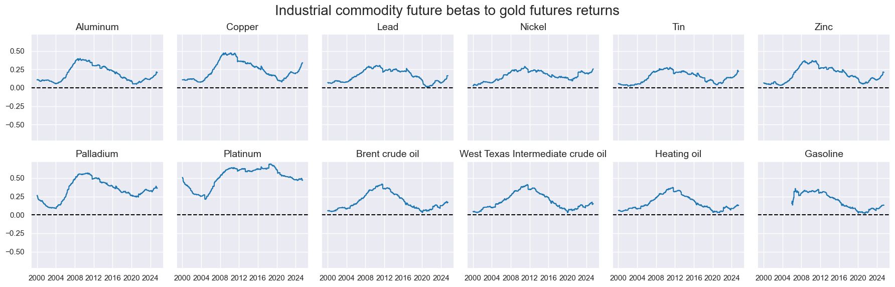
A simple way to partially hedge against this factor is to estimate the “gold beta” of individual volatility-targeted industrial commodity futures positions and take a corresponding offsetting position in the front-month gold futures. Although gold has limited industrial use relative to its dominant role in jewellery, its price is typically sensitive to inflation expectations and currency debasement concerns, which may also influence industrial commodity markets. The gold beta is estimated via a sequential regression, using a rolling 5-year lookback window, of the returns from volatility-targeted positions in individual industrial commodity contracts on the returns of a similarly volatility-targeted position in the gold futures contract. By this measure, all industrial contracts have always displayed positive sensitivity to gold’s performance since 2000.
The composite global surprise signal also predicts hedged basket positions positively and with near-100% probability of significance. Correlation coefficients have been somewhat higher, however, for the full sample and the two half samples.
On the whole, hedging would have produced a slightly higher risk-adjusted PnL without being a “game changer”. The long-term Sharpe ratio of the strategy with unbiased signal would have been 0.7 and the Sortino ratio 1.0, with virtually no correlation with the S&P500 returns and slightly lower seasonality than without hedging. Also, the advantage of the long-bias hedged strategy over the hedged long-only book has been greater than in the case of the unhedged strategy. Hedging generally reduces risk-adjusted PnL returns of long portfolios, however.
Annex 1: Economies for which economic surprises have been calculated
On JPMaQS, point-in-time metrics for industry growth and manufacturing survey surprise are available for 32 developed and emerging market economies (in alphabetical order of the currency ticker): Australia (AUD), Brazil (BRL), Canada (CAD), Switzerland (CHF), Chile (CLP), China (CNY), Colombia (COP), Czech Republic (CZK), the euro area (EUR), the UK (GBP), Hungary (HUF), Indonesia (IDR), Israel (ILS), India (INR), Japan (JPY), South Korea (KRW), Mexico (MXN), Malaysia (MYR), Norway (NOK), New Zealand (NZD), Peru (PEN), the Philippines (PHP), Poland (PLN), Romania (RON), Russia (RUB), Sweden (SEK), Singapore (SGD), Thailand (THB), Turkey (TRY), Taiwan (TWD), the U.S. (USD), and South Africa (ZAR). No suitable manufacturing survey is available in Thailand. Construction surveys are available for a subset of 22 countries. Availability is summarised in the exhibit below.


