Quantamental economic surprises are point-in-time measures of deviations of economic indicators from expected values. There are two types of surprises: first-print events and pure revisions. First-print events feature new observation periods, and the surprise element depends on market expectations of the indicator. Market surveys can approximate such expectations, but only for a limited number of indicators. Quantamental surprises use econometric prediction models and can be calculated for all indicators and transformations, principally using the whole information state.
This post introduces economic surprises in global industry and construction and shows how they can be transformed into short-term macro trading signals for commodities. There is clear empirical evidence for the predictive power of such surprises for a basket of industrial commodity futures at a daily and weekly frequency. Related simulated PnL generation produces risk-adjusted alpha, albeit mainly in seasons of large swings in manufacturing and construction.
The post below is based on Macrosynergy’s proprietary research. Please quote as “Brine, Eric, De la Porte Simonsen, Lasse and Sueppel, Ralph, ‘Economic surprise indicators: Primer and strategy example,” Macrosynergy research post, April 2025.”
A Jupyter notebook for audit and replication of the research results can be downloaded here. The notebook operation requires access to J.P. Morgan DataQuery to download data from JPMaQS. Everyone with DataQuery access can download data except for the latest months. Moreover, J.P. Morgan offers free trials on the complete dataset for institutional clients. An academic support program sponsors data sets for research projects.
Understanding quantamental economic surprises
Quantamental indicators are information states of market-relevant economic developments that are calculated for each date based on concurrently available economic time series. Changing time series are also called “vintages”. As a result, economic information states change whenever any of the underlying vintages change. This happens if either a new observation period is reported or if previously reported observation periods are revised.
Quantamental economic surprises are defined as point-in-time deviations of quantamental indicators from expected values. Expected values are estimated predictions of an informed market participant. Following this definition, two types of surprises jointly make up economic surprise indicators:
- A first-print event is the difference between a quantamental indicator on a release date and its expected value. A release date is the day on which any underlying economic time series adds a new observation period. Expected values must be estimated, typically based on econometric models and information prior to the release date. A quantamental data surprise is always specific to the prediction model and its statistical learning process.
- A pure revision event is the change in a quantamental indicator on a non-release date. It arises from revisions of data for previously released observation periods. By default, we assume that all revisions are surprises, i.e., that the latest reported value for an observation period is the best predictor of its value after revisions. Note that any revisions published on a release date become part of the first print event.
A quantamental indicator of economic surprises records the values of these two events on their publication dates. It records zero values for all other dates. Models that predict indicators on release dates must always use the latest prior vintage of the underlying data series. Predictive models are typically applied to stationary increments, i.e., differences or log differences of volume, value or price indices. The predicted next increment produces an expected new vintage, and the expected new vintage implies a new derived expected quantamental indicator, such as an annual growth rate or moving average. Note that in this way, predictions automatically account for “base effects”, i.e., predictable changes in growth rates that arise from unusually sharp increases or declines in index levels of the base period, for example, a year ago.
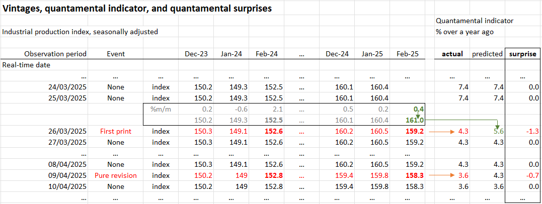
The process of increment prediction and implied indicator surprises is demonstrated in the graph below for the example of industrial production. The quantamental indicator is the daily information state of the latest production growth as a percentage over a year ago (column “actual” in the graph below). For each real-time date, the growth rate is calculated based on the concurrent vintage of a seasonally adjusted index (“index” rows below). On dates when the vintage does not change, the quantamental surprise indicator delivers values of zero. On a release date (say the 25th of March), the surprise indicator considers a predicted quantamental indicator and subtracts it from the actual new quantamental indicator. The prediction is based on the estimated increment of the added month (February) using the time series of previous increments through January 2025. Jointly, the old vintage and the new predicted index give a predicted new vintage. The predicted indicator is calculated based on that vintage and subtracted from the one based on the actual new vintage. On a revision date (say April 9), the surprise indicator simply uses the change in the quantamental indicator as a surprise.
Quantamental indicators can be based on more than one underlying economic data series. This means that they may be calculated by using two or more sets of vintages. In this case, the quantamental indicator and its surprises may be subject to multiple first-print events.
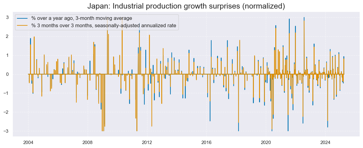
The chart below illustrates the nature of quantamental economic surprise indicators, which use surprises to show industrial production growth in Japan over the past 20 years. There have typically been two surprises per month, reflecting first-print events and revisions. Note that if the market watches more than one type of growth rate, say a short-term growth rate and an annual growth trend, those may show different surprises. For example, in the case of upward revisions to recent production levels and downward revisions to previous months, there may be positive surprises to short-term growth rates without much impact on annual growth rates. The surprise perspective depends on the strategy that one wishes to design.
In the above example and further in this post, predictions of increments for release dates have been estimated with an ARMA(1,1) model. This simple univariate time series model predicts increments based on an autoregressive component, i.e., the effect of the last period’s value, and a moving average component, represented by the last period’s error. The coefficients of the model are estimated sequentially based on the vintages of production indices. And each vintage-specific model produces a one-step-ahead forecast for the subsequent observation period. Surprises against these forecasts would be called ARMA(1,1) surprises, and these are used for the commodity futures trading strategy below.
How quantamental surprises differ from conventional surprise indicators
Standard economic surprise indicators, such as those of Citigroup or Bloomberg, are based on differences between released economic indicators and predictions according to economist surveys. Thus, they are calculated exclusively for release dates and for indicators that are part of market surveys. These surprise metrics have the advantage of using actual predictions that are published along data release calendars and that influence many traders’ expectations. However, quantamental economic surprises have a slightly different purpose and offer their own practical advantages:
- Quantamental economic surprises are measured against clearly defined benchmarks, i.e., prediction models that are continually updated by using the latest information. Economist surveys are of very different quality, depending on indicators, country, and forecasting institution. Indeed, for less critical data releases, filling in survey forms can be pretty perfunctory. Also, surveys are not updated continuously as the information space changes.
- Quantamental surprises can be measured for any indicator and transformation of interest, not just those that market news agencies survey. For example, general government accounts, international investment positions, or bank lending conditions are not regularly part of data release calendars. Also, market news agencies do not survey various types of short-term growth rates in activity indicators, even though they are analytically valuable. This means that quantamental economic surprises can be tailored to a specific investment strategy.
- Quantamental economic surprises include all pure revision events, including those that are not scheduled in Bloomberg’s or other market calendars. Revisions occur due to additional information for an observation period, methodology changes, and error corrections. There are also comprehensive “benchmark revisions” that include information that is not available at high frequency at a later point in time. Revisions can significantly alter perceptions of the economy.
- Quantamental surprises can principally be divided into volatility and actual trend changes, as long as sources of volatility are identified. The latter include working day effects, weather effects, and changes in holiday patterns, such as those related to the Chinese New Year and Easter. Only surprises that are not related to temporary effects are indicative of trend changes.
Example: Surprises to the global industry cycle
As an example, we look at quantamental metrics of surprises to global industry and construction growth, using ARMA(1,1) models to predict period ahead increments of output or survey levels. These types of surprises have recently been added to the J.P. Morgan Macrosynergy Quantamental System (“JPMaQS). The indicators whose surprises are used in this post are the following:
- Industrial production: Surprises are calculated for three growth rates, [1] % over a year ago as 3-month moving average, [2] % 6 months over the previous 6 months, seasonally adjusted and annualized, and [3] % 3 months over the previous 3 months, seasonally adjusted and annualized (documentation here).
- Manufacturing business confidence: Surprises are calculated for the seasonally adjusted level of local manufacturing confidence scores as well as for two rates of change: the difference of the last 6 months over the previous 6 months and the difference of the last 3 months over the previous 3 months (documentation here).
- Construction business confidence: Surprises are calculated for the seasonally adjusted level of local construction confidence scores as well as for the same two rates of change as the ones used for manufacturing confidence (documentation here).
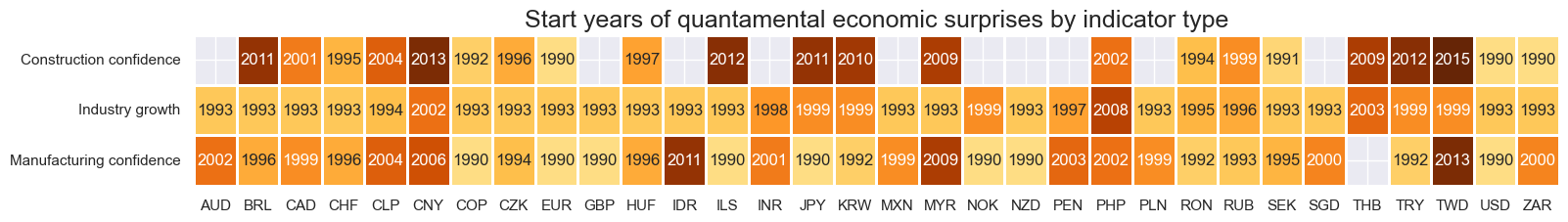
On JPMaQS, point in time metrics for industry growth and manufacturing survey surprise are available for 32 developed and emerging market economies (in alphabetical order of the currency ticker): Australia (AUD), Brazil (BRL), Canada (CAD), Switzerland (CHF), Chile (CLP), China (CNY), Colombia (COP), Czech Republic (CZK), the euro area (EUR), the UK (GBP), Hungary (HUF), Indonesia (IDR), Israel (ILS), India (INR), Japan (JPY), South Korea (KRW), Mexico (MXN), Malaysia (MYR), Norway (NOK), New Zealand (NZD), Peru (PEN), the Philippines (PHP), Poland (PLN), Romania (RON), Russia (RUB), Sweden (SEK), Singapore (SGD), Thailand (THB), Turkey (TRY), Taiwan (TWD), the U.S. (USD), and South Africa (ZAR). Construction surveys are available for a subset of 22 countries. Availability is summarized in the exhibit below.
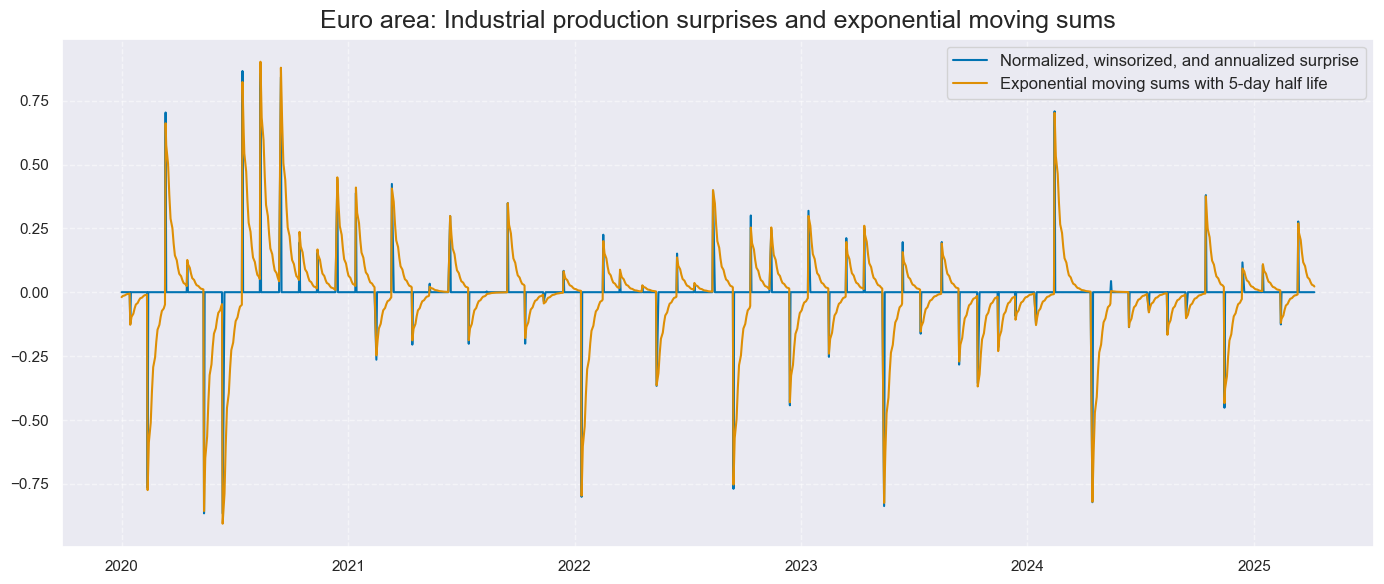
For the generation of trading signals, quantamental economic surprises typically need to be normalized, winsorized, and annualized. This is essential if we want to compute composite surprise indicators across economic indicators and countries. These three steps must carefully consider the nature of the time series of quantamental economic surprises:
- Normalization here means division of each surprise value by point-in-time standard deviations of its own first print events. Standard deviations of pure revisions are typically lower and a less intuitive denominator. The zero values of non-release and non-revision dates are irrelevant and must not be considered for normalization.
- Winsorization means containing absolute values of surprises to de-emphasize data distortions and extreme events. Here, we capped all values at three standard deviations on the negative and positive side.
- Annualization here means the transformation of surprises into annual units. Quarterly-frequency data convey more information than monthly ones, as they cover longer periods. To equalize the information value of indicators of different frequencies, we divide by the square root of the number of observation periods in the year, assuming that an unbiased discrete random walk roughly approximates those changes.
The normalized, winsorized and annualized surprises are then aggregated to a single global industry surprise indicator in four steps:
- Conceptual aggregation: The normalized surprises of all different derivatives of a single indicator, say, industrial production, can be combined into one by average. This means we condense all information into three metrics: an industrial production surprise, a manufacturing confidence surprise and a construction confidence surprise.
- Temporal aggregation: Surprise effects are unlikely to evaporate instantaneously. Hence, we calculate moving sums with 3-day and 5-day half-lives. This means that information is mostly absorbed over the course of a week or two, which corresponds with the frequency of many research reports and briefings.
- Geographical aggregation: We form weighted moving averages, using as weights point-in-time series of industrial value-added in USD for the 32 economies. The aggregation results in three global surprise indicators with ample short-term variability and cyclical variation.
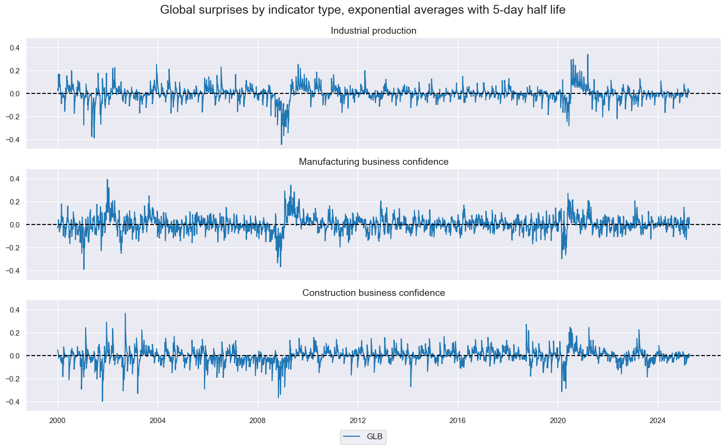
- Final composite aggregation: Finally, we can form unweighted averages of the three types of surprise into a single global industry and construction activity surprise. We do so for 3-day and 5-day moving sums of the underlying daily surprises.
Altogether, aggregation usually increases the autocorrelation of quantamental economic surprise indicators. Temporal aggregation naturally introduces serial correlation. Conceptual and global aggregation that combines related economic phenomena often reveal meaningful global surprise trends.
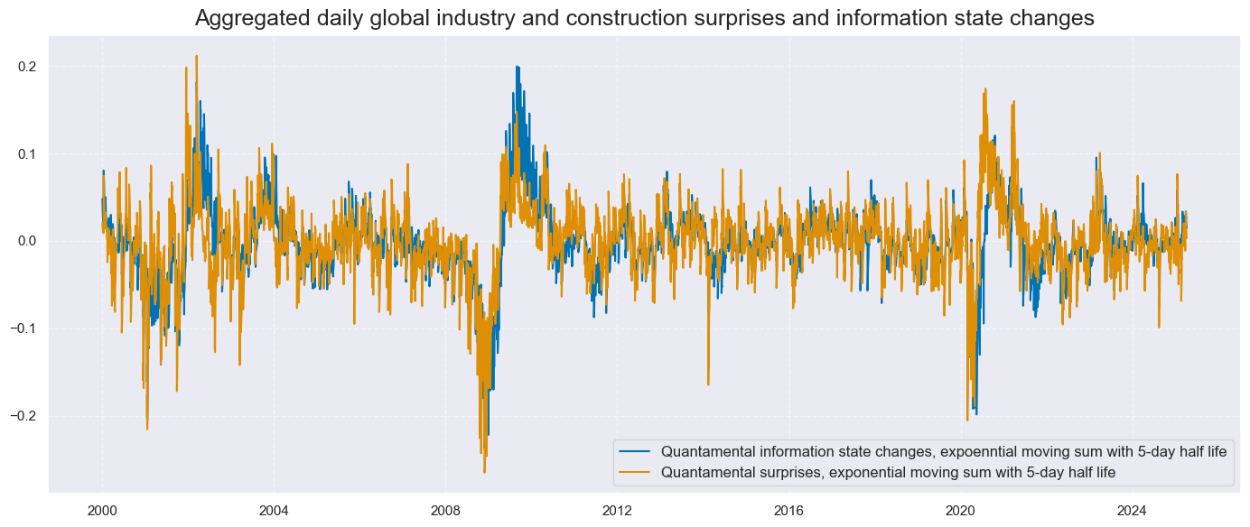
As a reference for some empirical analyses, we also calculate the simpler information state changes for the above indicators in the same way (view previous post Macro information changes as systematic trading signals). Macro information state changes are point-in-time updates of recorded economic developments. They can be calculated directly from any point-in-time quantamental indicator and do not require separate data series from the J.P. Morgan Macrosynergy Quantamental System.
Surprises and information state changes in the global industry have common but not identical patterns. Surprises seem to be leading in recessions and recoveries. Moreover, information state changes do not account for “base effects”, i.e., changes in annual growth rates that reflect large jumps and drops a year earlier.
Application: Trading industrial commodities based on economic surprises
We apply global surprises to a very simple strategy based on a single idea. All other things equal, positive surprises in industry, manufacturing and construction data should precede upward revisions of industrial commodity demand estimates. Thereby, they should positively predict returns on futures for industrial commodities. The strategy trades only one position: a risk-parity basket of the following commodity futures: LME aluminum, Comex copper, LME lead, LME tin, LME nickel, LME zinc, NYMEX palladium, NYMEX platinum, ICE Brent crude, NYMEX WTI light crude, NYMEX RBOB Gasoline, and NYMEX Heating oil (New York Harbor). We approximate the returns of the basket by using an average of generic volatility-adjusted returns of JPMaQS (documentation here).
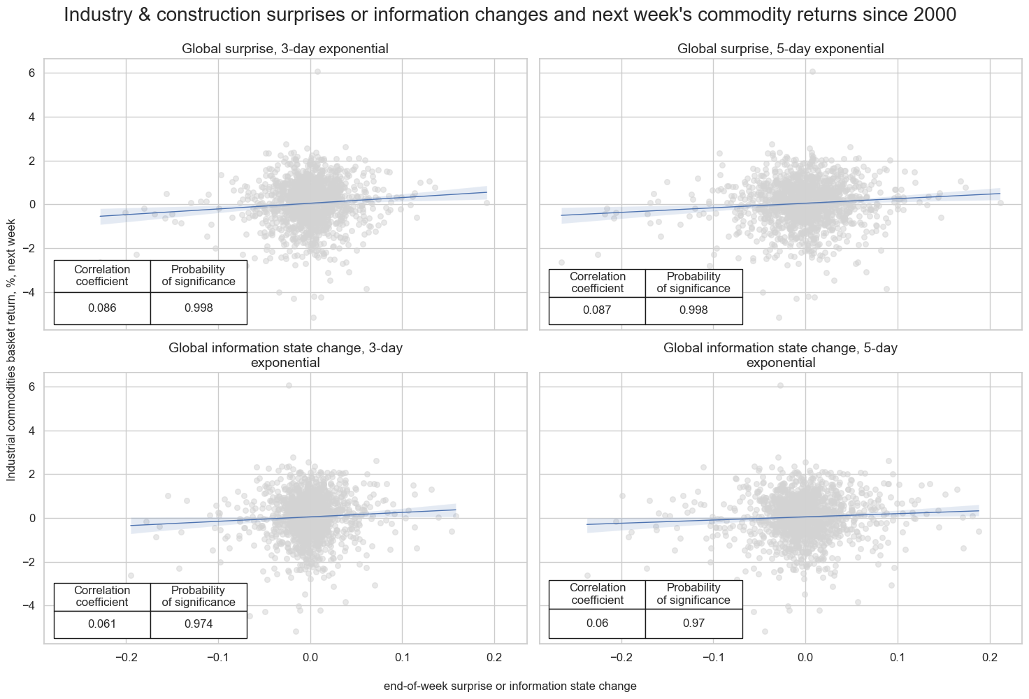
There is clear empirical confirmation of the positive predictive power of industry and construction surprises with respect to subsequent commodity futures returns at daily, weekly or monthly frequencies since 2000. The predictive relation has been highly significant, and surprises have posted higher forward correlation with returns than mere information state changes.
Similarly, the accuracy and balanced accuracy of economic surprises with respect to subsequent daily, weekly, and monthly returns have consistently been above 50%. Even daily, accuracy has been over 51% since 2000.
Finally, we assess the economic value of a primitive strategy that simply takes a position at the end of each day in proportion to the global economic surprise indicators of that day (up to a maximum of 3 standard deviations of its normalized value). The naïve PnL does not consider transaction costs or compounding. For charting, the PnL has been scaled to an annualized volatility of 10%. The long-term Sharpe ratio of any of the two economic surprise signals would have been around 0.7 and the Sortino ratio 1.0-1.1. Signals would have had a slight short bias, and correlation with the S&P500 would have been slightly negative.
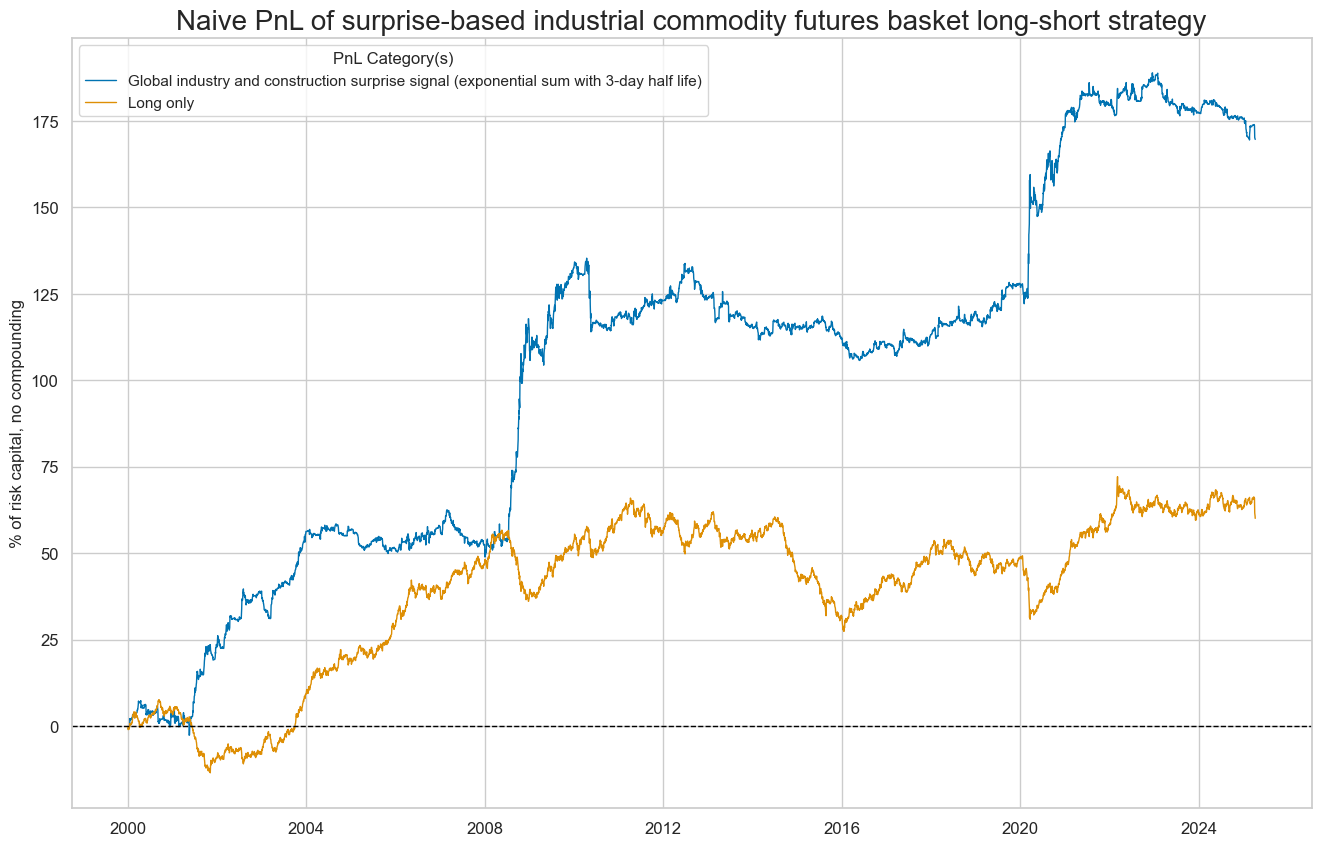
PnL generation has been extremely seasonal, focusing on periods of economic recession and recovery. About 85% of the last 25 years’ PnL has been earned in the top 5% of traded months. However, high seasonality is to be expected from a strategy that uses a single-principle signal and trades only a single position. For example, the PnL profile looks highly complementary to those we have previously shown for inventory signals (see previous post “Inventory scores and metal futures returns”).


