Cross-country equity futures strategy #
This notebook illustrates the concepts discussed in the post “Cross-country Equity Futures Strategies” available on the Macrosynergy website.
The notebook evaluates five simple thematic and potentially differentiating macro scores across a panel of 16 developed and emerging markets. It demonstrates that even a basic, non-optimized composite score could have added substantial value beyond a risk-parity exposure to global equity index futures. Additionally, a purely relative value equity index futures strategy would have provided respectable long-term returns, complementing passive equity exposure.
The notebook explores both directional and relative equity futures strategies, including:
-
Global Directional Futures Strategy,
-
Directional Futures Strategy for Developed Markets,
-
Global Relative Futures Strategy, and
-
Relative Futures Strategy for Developed Markets
Get packages and JPMaQS data #
# >>> Define constants <<< #
import os

# Retrieve credentials
client_id: str = os.getenv("DQ_CLIENT_ID")
client_secret: str = os.getenv("DQ_CLIENT_SECRET")

# Define any Proxy settings required (http/https)
PROXY = {}

# Start date for the data (argument passed to the JPMaQSDownloader class)
START_DATE = "2000-01-01"
import numpy as np
import pandas as pd
import matplotlib.pyplot as plt

import warnings
import os
from datetime import date

import macrosynergy.management as msm
import macrosynergy.panel as msp
import macrosynergy.signal as mss
import macrosynergy.pnl as msn
import macrosynergy.visuals as msv
from macrosynergy.download import JPMaQSDownload

warnings.simplefilter("ignore")
The JPMaQS indicators we consider are downloaded using the J.P. Morgan Dataquery API interface within the
macrosynergy
package. This is done by specifying ticker strings, formed by appending an indicator category code
DB(JPMAQS,<cross_section>_<category>,<info>)
, where
value
giving the latest available values for the indicator
eop_lag
referring to days elapsed since the end of the observation period
mop_lag
referring to the number of days elapsed since the mean observation period
grade
denoting a grade of the observation, giving a metric of real time information quality.
After instantiating the
JPMaQSDownload
class within the
macrosynergy.download
module, one can use the
download(tickers,start_date,metrics)
method to easily download the necessary data, where
tickers
is an array of ticker strings,
start_date
is the first collection date to be considered and
metrics
is an array comprising the times series information to be downloaded. For more information see
here
# Cross-sections of interest

cids_dmeq = ["AUD", "CAD", "CHF", "EUR", "GBP", "JPY", "SEK", "USD"]
cids_eueq = ["DEM", "ESP", "FRF", "ITL", "NLG"]
cids_aseq = ["CNY", "HKD", "INR", "KRW", "MYR", "SGD", "THB", "TWD"]
cids_exeq = ["BRL", "TRY", "ZAR"]
cids_nueq = ["MXN", "PLN"]

cids_eq = sorted(cids_dmeq + cids_eueq + cids_aseq + cids_exeq + cids_nueq)
cids_eqxe = sorted(list(set(cids_eq) - set(cids_eueq)))
cids_eqxx = sorted(list(set(cids_eqxe) - set(["CNY", "TRY", "PLN", "HKD", "SGD"])))
cids_eqxu = sorted(list(set(cids_eqxx) - set(["USD"])))
cids = cids_eq
# Category tickers

inf = [
    "CPIH_SA_P1M1ML12",
    "CPIH_SJA_P6M6ML6AR",
    "CPIC_SA_P1M1ML12",
    "CPIC_SJA_P6M6ML6AR",
    "INFTEFF_NSA",
]
lab = [
    "EMPL_NSA_P1M1ML12_3MMA",
    "EMPL_NSA_P1Q1QL4",
    "UNEMPLRATE_NSA_3MMA_D1M1ML12",
    "UNEMPLRATE_NSA_D1Q1QL4",
    "WFORCE_NSA_P1Y1YL1_5YMA",
    "WFORCE_NSA_P1Q1QL4_20QMM",
]
ofx = [
    "REEROADJ_NSA_P1M1ML12",
    "NEEROADJ_NSA_P1M1ML12",
    "REER_NSA_P1M1ML12",
]
fin = [
    "RIR_NSA",
    "FXCRR_NSA",
    "EQCRR_NSA",
]
tot = [
    "CTOT_NSA_P1M1ML12",
    "MTOT_NSA_P1M1ML12",
]
add = [
    "RGDP_SA_P1Q1QL4_20QMM",
]

eco = inf + lab + ofx + fin + tot + add

mkt = [
    "EQXR_NSA",
    "EQXR_VT10",
    "FXTARGETED_NSA",
    "FXUNTRADABLE_NSA",
]

xcats = eco + mkt

# Resultant indicator tickers

tickers = [cid + "_" + xcat for cid in cids_eq for xcat in xcats]
print(f"Maximum number of tickers is {len(tickers)}")
Maximum number of tickers is 624
The description of each JPMaQS category is available either under Macro Quantamental Academy , or on JPMorgan Markets (password protected). In particular, the set used for this notebook is using Consumer price inflation trends , Inflation targets , Labor market dynamics , Demographic trends , Openness-adjusted effective appreciation , Equity index future carry , FX forward carry , Real interest rates , GDP growth , Terms-of-trade , Equity index future returns , and FX tradeability and flexibility
# Download from DataQuery
with JPMaQSDownload(
    client_id=client_id, client_secret=client_secret
) as downloader:
    df: pd.DataFrame = downloader.download(
        tickers=tickers,
        start_date=START_DATE,
        metrics=["value"],
        suppress_warning=True,
        show_progress=True,
        report_time_taken=True,
        proxy=PROXY,
    )
Downloading data from JPMaQS.
Timestamp UTC:  2025-06-25 12:36:03
Connection successful!
Requesting data: 100%|██████████| 32/32 [00:06<00:00,  4.92it/s]
Downloading data: 100%|██████████| 32/32 [00:24<00:00,  1.33it/s]
Time taken to download data: 	32.03 seconds.
Some expressions are missing from the downloaded data. Check logger output for complete list.
147 out of 624 expressions are missing. To download the catalogue of all available expressions and filter the unavailable expressions, set `get_catalogue=True` in the call to `JPMaQSDownload.download()`.
dfx = df.copy()
dfx.info()
<class 'pandas.core.frame.DataFrame'>
RangeIndex: 3029408 entries, 0 to 3029407
Data columns (total 4 columns):
 #   Column     Dtype
---  ------     -----
 0   real_date  datetime64[ns]
 1   cid        object
 2   xcat       object
 3   value      float64
dtypes: datetime64[ns](1), float64(1), object(2)
memory usage: 92.5+ MB
Availability and renaming #
The
check_availability()
function in
macrosynergy.management
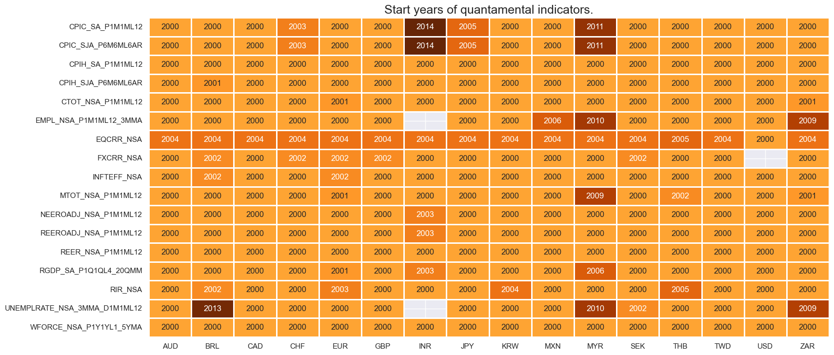
displays the start dates from which each category is available for each requested country, as well as missing dates or unavailable series.
xcatx = inf
msm.check_availability(df=df, xcats=xcatx, cids=cids, missing_recent=False)

xcatx = lab
msm.check_availability(df=df, xcats=xcatx, cids=cids, missing_recent=False)

xcatx = ofx + tot
msm.check_availability(df=df, xcats=xcatx, cids=cids, missing_recent=False)

xcatx = fin
msm.check_availability(df=df, xcats=xcatx, cids=cids, missing_recent=False)

xcatx = mkt
msm.check_availability(df=df, xcats=xcatx, cids=cids, missing_recent=False)

Renaming #
For the purpose of the below presentation, we have renamed quarterly-frequency indicators to approximate monthly equivalents in order to have a full panel of similar measures across most countries. The two series are not identical but are close substitutes.
# Unify quarterly and 3-month moving average names

dict_repl = {
    "EMPL_NSA_P1Q1QL4": "EMPL_NSA_P1M1ML12_3MMA",
    "WFORCE_NSA_P1Q1QL4_20QMM": "WFORCE_NSA_P1Y1YL1_5YMM",
    "UNEMPLRATE_NSA_D1Q1QL4": "UNEMPLRATE_NSA_3MMA_D1M1ML12",
    "UNEMPLRATE_SA_D1Q1QL1": "UNEMPLRATE_SA_D3M3ML3",
}

for key, value in dict_repl.items():
    dfx["xcat"] = dfx["xcat"].str.replace(key, value)
# Display availability of re-named and unified indicators

xcatx = eco
msm.check_availability(df=dfx, xcats=xcatx, cids=cids_eqxx, missing_recent=False)
Blacklisting #
Before running the analysis, we use
make_blacklist()
helper function from
macrosynergy
package, which creates a standardized dictionary of blacklist periods, i.e. periods that affect the validity of an indicator, based on standardized panels of binary categories.
Put simply, this function allows converting category variables into blacklist dictionaries that can then be passed to other functions. Below, we picked two indicators for FX tradability and flexibility.
FXTARGETED_NSA
is an exchange rate target dummy, which takes a value of 1 if the exchange rate is targeted through a peg or any regime that significantly reduces exchange rate flexibility and 0 otherwise.
FXUNTRADABLE_NSA
is also a dummy variable that takes the value one if liquidity in the main FX forward market is limited or there is a distortion between tradable offshore and untradable onshore contracts.
# Create blacklisting dictionary

dfb = df[df["xcat"].isin(["FXTARGETED_NSA", "FXUNTRADABLE_NSA"])].loc[
    :, ["cid", "xcat", "real_date", "value"]
]
dfba = (
    dfb.groupby(["cid", "real_date"])
    .aggregate(value=pd.NamedAgg(column="value", aggfunc="max"))
    .reset_index()
)
dfba["xcat"] = "FXBLACK"
fxblack = msp.make_blacklist(dfba, "FXBLACK")
fxblack
{'BRL': (Timestamp('2012-12-03 00:00:00'), Timestamp('2013-09-30 00:00:00')),
 'CHF': (Timestamp('2011-10-03 00:00:00'), Timestamp('2015-01-30 00:00:00')),
 'CNY': (Timestamp('2000-01-03 00:00:00'), Timestamp('2025-06-24 00:00:00')),
 'HKD': (Timestamp('2000-01-03 00:00:00'), Timestamp('2025-06-24 00:00:00')),
 'INR': (Timestamp('2000-01-03 00:00:00'), Timestamp('2004-12-31 00:00:00')),
 'MYR_1': (Timestamp('2000-01-03 00:00:00'), Timestamp('2007-11-30 00:00:00')),
 'MYR_2': (Timestamp('2018-07-02 00:00:00'), Timestamp('2025-06-24 00:00:00')),
 'SGD': (Timestamp('2000-01-03 00:00:00'), Timestamp('2025-06-24 00:00:00')),
 'THB': (Timestamp('2007-01-01 00:00:00'), Timestamp('2008-11-28 00:00:00')),
 'TRY_1': (Timestamp('2000-01-03 00:00:00'), Timestamp('2003-09-30 00:00:00')),
 'TRY_2': (Timestamp('2020-01-01 00:00:00'), Timestamp('2024-07-31 00:00:00'))}
Transformations and checks #
Thematic feature groups #
Inflation shortfall #
Most quantamental indicators that professional investment managers would deploy require careful customization and transformations of original JPMaQS data. Since all quantamental data are standardized information states over a range of countries, transformations are simple.
The
panel_calculator()
function in
macrosynergy.panel
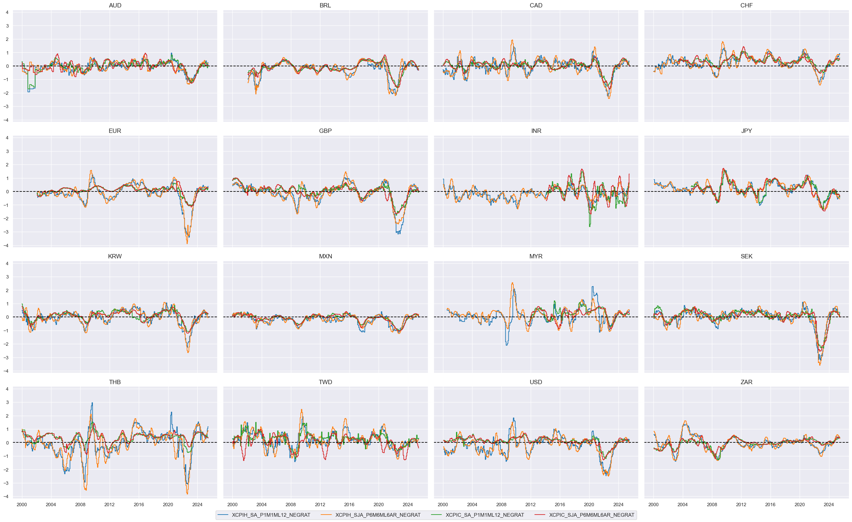
makes it easy and intuitive to apply a wide range of transformations to each cross section of a panel by using a string. Below we calculate plausible metrics of excess inflation versus a country’s effective inflation target.
update_df()
function adds the new indicators to the original dataframe
dfx
.
# Calculate negative excess inflation rates

# Preparation: for relative target deviations, we need denominator bases that should never be less than 2
infs = [i for i in inf if i[:5] in ["CPIH_", "CPIC_"]]
xcatx = infs
cidx =cids_eqxx

# calculate negative excess inflation rates
calcs = []
calcs += ["INFTEBASIS = INFTEFF_NSA.clip(lower=2) "]
for xc in xcatx:
    calcs += [f"X{xc}_NEG = - {xc} + INFTEFF_NSA "]
    calcs += [f"X{xc}_NEGRAT = X{xc}_NEG / INFTEBASIS "]

dfa = msp.panel_calculator(dfx, calcs=calcs, cids=cidx)
dfx = msm.update_df(dfx, dfa)

# Collect in factor dictionary
dict_factors = {}  # Create dictionary to store factors

xinfs = list(dfa['xcat'].unique())
xinf_negs = [x for x in xinfs if x.endswith("_NEGRAT")]
dict_factors["XINF_NEG"] = xinf_negs
The macrosynergy package provides two useful functions,
view_ranges()
and
view_timelines()
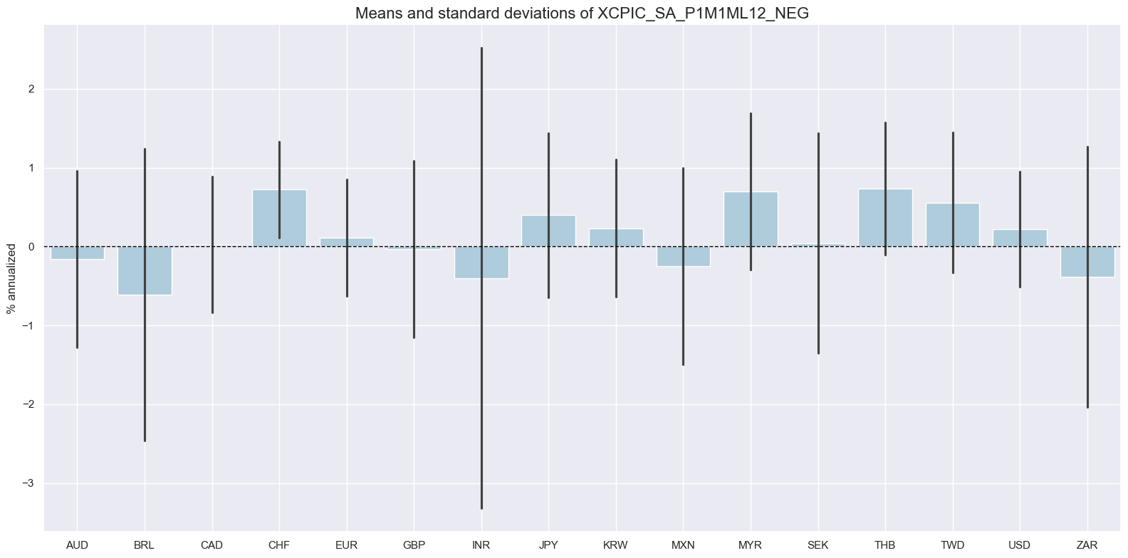
, which assist in plotting means, standard deviations, and time series of the chosen indicators.
cidx = cids_eqxx
xcatx = [x for x in xinfs if x.startswith("XCPIC_SA_P1M1ML12")]

msp.view_ranges(
    dfx,
    xcats=[xcatx[0]],
    kind="bar",
    title=f"Means and standard deviations of {xcatx[0]}",
    ylab="% annualized",
    start="2000-01-01",
)
cidx = cids_eqxx
xcatx = xinf_negs

msp.view_timelines(
    dfx,
    xcats=xcatx,
    cids=cidx,
    ncol=4,
    start="2000-01-01",
    same_y=True,
)
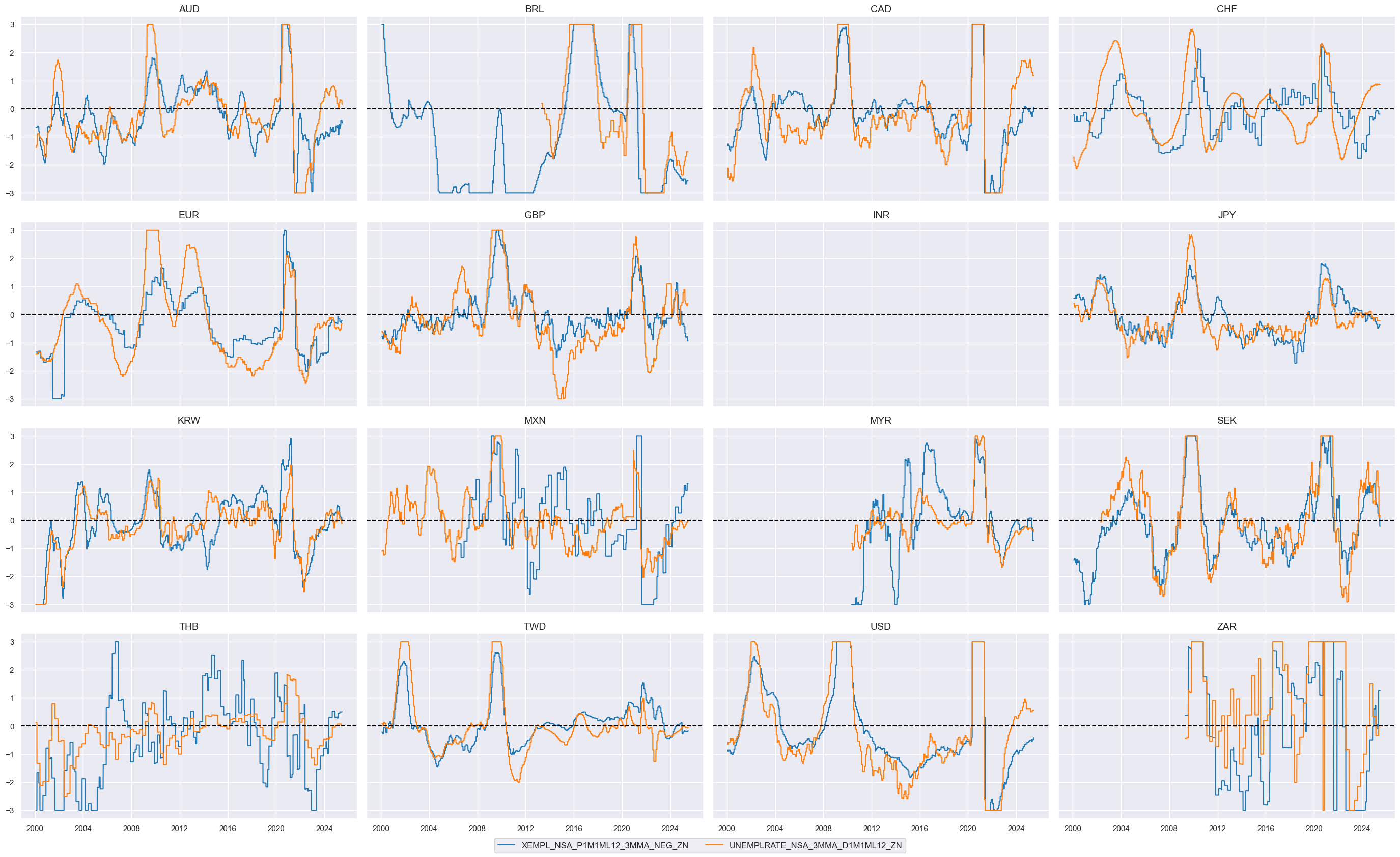
Labor market slackening #
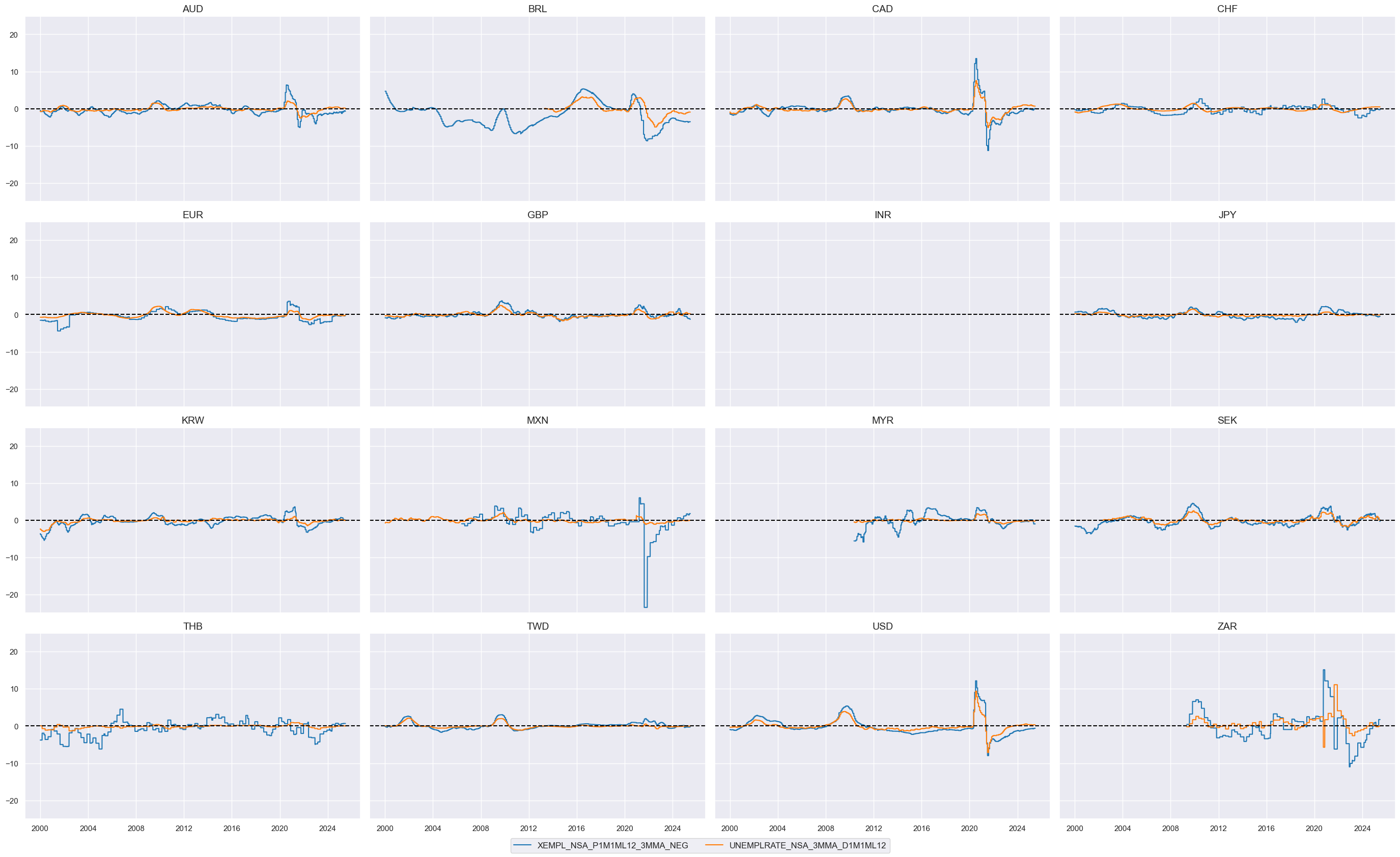
To understand how the business cycle affects employment growth, we measure the deviation of current employment growth from the long-term workforce median, known as “excess employment growth.” This isolates the portion of growth due to the business cycle, revealing deviations from the long-term trend. The following cell calculates the negative of “excess employment growth” to analyze the impact of negative deviations.
# Calculate indicators of labor market tightening or tightness

cidx = cids_eqxx

calcs = [
    "XEMPL_NSA_P1M1ML12_3MMA_NEG = - EMPL_NSA_P1M1ML12_3MMA + WFORCE_NSA_P1Y1YL1_5YMA",
]

dfa = msp.panel_calculator(dfx, calcs=calcs, cids=cidx)
dfx = msm.update_df(dfx, dfa)

# Collect in factor dictionary

lab_slacks = [
    "XEMPL_NSA_P1M1ML12_3MMA_NEG",
    "UNEMPLRATE_NSA_3MMA_D1M1ML12",
]
dict_factors["LAB_SLACK"] = lab_slacks
cidx = cids_eqxx
xcatx = lab_slacks

msp.view_timelines(
    dfx,
    xcats=xcatx,
    cids=cidx,
    ncol=4,
    start="2000-01-01",
    same_y=True,
)
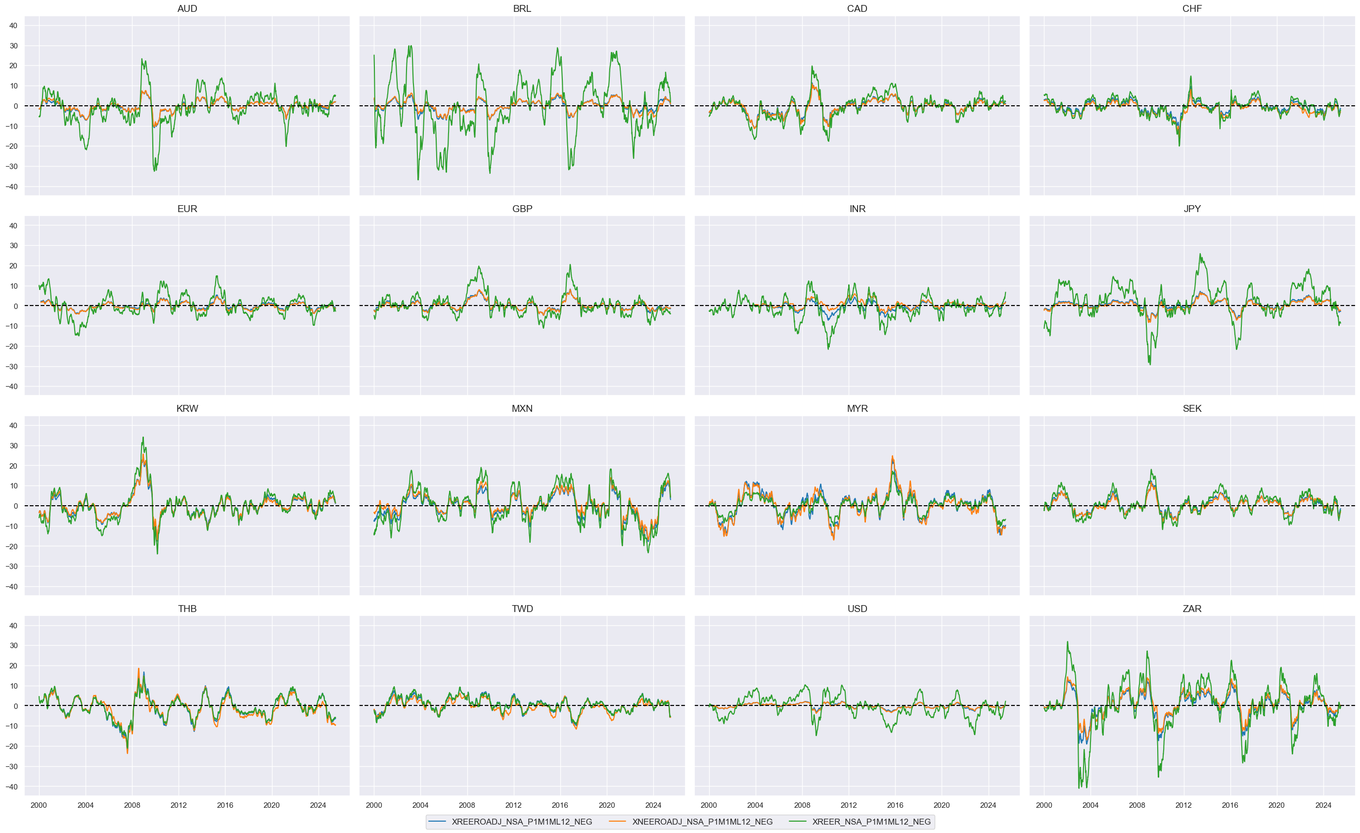
Effective currency depreciation #
# Calculate the negatives of openness-adjusted effective real appreciation collected previously in the list ofx

xcatx = ofx
cidx = cids_eqxx

calcs = []
for xc in xcatx:
    calc = [f"X{xc}_NEG = - {xc}"]
    calcs.extend(calc)

dfa = msp.panel_calculator(dfx, calcs=calcs, cids=cidx)
dfx = msm.update_df(dfx, dfa)

# Collect in factor dictionary

fx_deprecs = list(dfa['xcat'].unique())
dict_factors["FX_DEPREC"] = fx_deprecs
cidx = cids_eqxx
xcatx = fx_deprecs

msp.view_timelines(
    dfx,
    xcats=xcatx,
    cids=cidx,
    ncol=4,
    start="2000-01-01",
    same_y=True,
)
Ease of local finance #
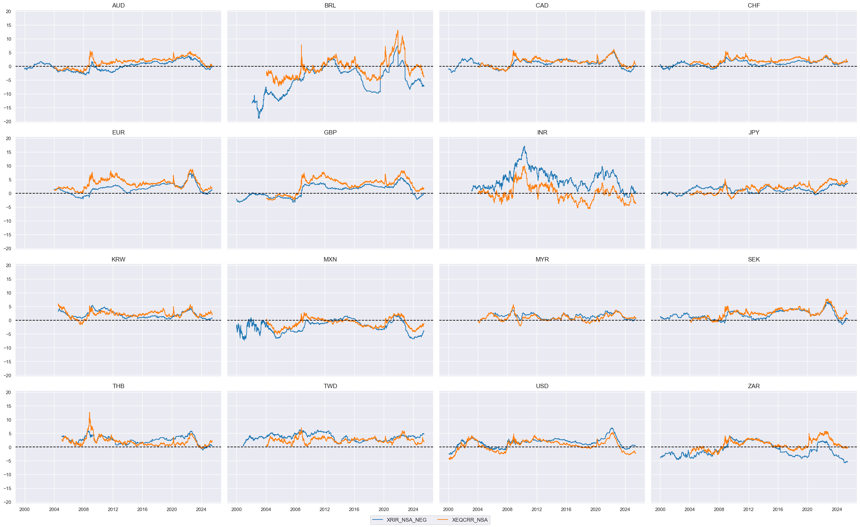
The idea behind this theme is simply that accommodative local financial conditions support demand for equity. The theme is represented by two indicators:
-
The first is the negative of an excess real short-term interest rate, which is calculated as the difference between a real expectations-based short-term interest rate (view documentation) and estimated productivity growth, whereby the latter is approximated by the difference between a GDP growth trend and work force growth trend .
-
The second indicators excess real equity carry based on the difference between (i) average of expected forward dividend and earnings yield and (ii) the main local-currency real short-term interest rate, in % annualized of notional of the contract (view documentation). Excess here means above 3.5%, a judgment call assuming that for equity carry to be attractive it needs to excess at least 20% of long-term average index future volatility.
# Calculate ease-of-financing indicators
cidx = cids_eqxx

calcs = [
    "XRIR_NSA_NEG = - RIR_NSA + RGDP_SA_P1Q1QL4_20QMM - WFORCE_NSA_P1Y1YL1_5YMA",
    "XEQCRR_NSA = EQCRR_NSA - 0.2 * 17.5"  # excess carry assuming equity vol of 17.5% and 0.2 minimum Sharpe
]

dfa = msp.panel_calculator(dfx, calcs=calcs, cids=cidx)
dfx = msm.update_df(dfx, dfa)

# Collect in factor dictionary

ease_fins = list(dfa['xcat'].unique())
dict_factors["EASE_FIN"] = ease_fins
cidx = cids_eqxx
xcatx = ease_fins

msp.view_timelines(
    dfx,
    xcats=xcatx,
    cids=cidx,
    ncol=4,
    start="2000-01-01",
    same_y=True,
)
Terms-of-trade improvement #
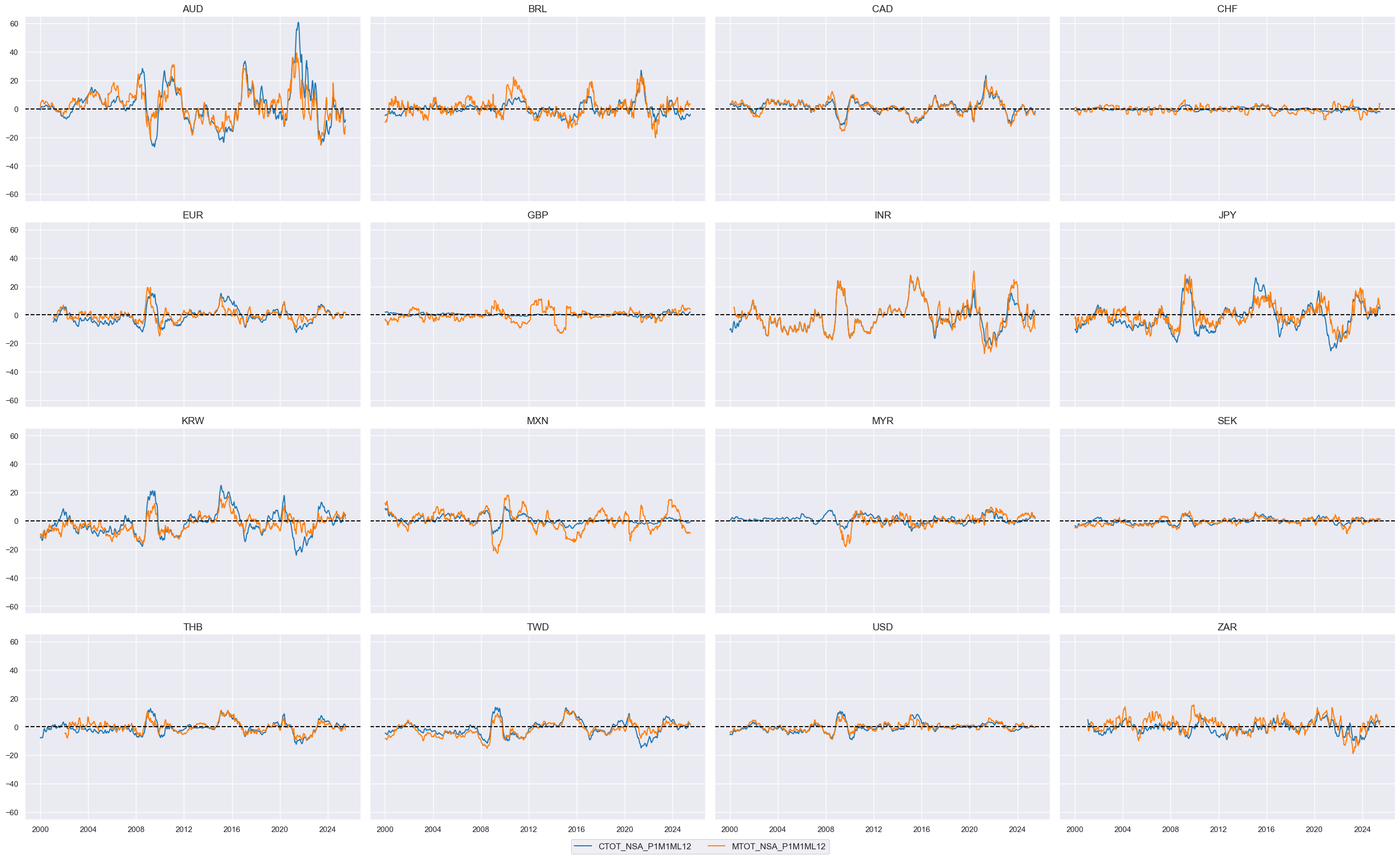
The indicators for terms of trade improvement are directly accessible on JPMaQS and do not need any adjustments.
# Use annual terms-of-trade growth
tot_poya = ["CTOT_NSA_P1M1ML12", "MTOT_NSA_P1M1ML12"]

dict_factors["TOT_POYA"] = tot_poya
cidx = cids_eqxx
xcatx = tot_poya

msp.view_timelines(
    dfx,
    xcats=xcatx,
    cids=cidx,
    ncol=4,
    start="2000-01-01",
    same_y=True,
)
Composite features #
Thematic scores #
The
make_zn_scores()
function is a method for normalizing values across different categories. This is particularly important when summing or averaging categories with different units and time series properties. The function computes z-scores for a category panel around a specified neutral level that may be different from the mean. The term “zn-score” refers to the normalized distance from the neutral value.
The default mode of the function calculates scores based on sequential estimates of means and standard deviations, using only past information. This is controlled by the
sequential=True
argument, and the minimum number of observations required for meaningful estimates is set with the
min_obs
argument. By default, the function calculates zn-scores for the initial sample period defined by
min_obs
on an in-sample basis to avoid losing history.
The means and standard deviations are re-estimated daily by default, but the frequency of re-estimation can be controlled with the
est_freq
argument, which can be set to weekly, monthly, or quarterly.
# Normalize thematic group members

cidx = cids_eqxx

xcatx = []
for key, value in dict_factors.items():
    xcatx.extend(value)  # list of all categories


dfa = pd.DataFrame(columns=list(dfx.columns))

for xc in xcatx:
    dfaa = msp.make_zn_scores(
        dfx,
        xcat=xc,
        cids=cidx,
        sequential=True,
        min_obs=261 * 5,
        neutral="zero",
        pan_weight=1,  # assumes comparable impact scales across cross-sections
        thresh=3,
        postfix="_ZN",
        est_freq="m",
    )
    dfa = msm.update_df(dfa, dfaa)

dfx = msm.update_df(dfx, dfa)
cidx = cids_eqxx
xcatx = [x + "_ZN" for x  in lab_slacks]  # dict_factors.keys()
msp.view_timelines(
    dfx,
    xcats=xcatx,
    cids=cidx,
    ncol=4,
    start="2000-01-01",
    same_y=True,
)
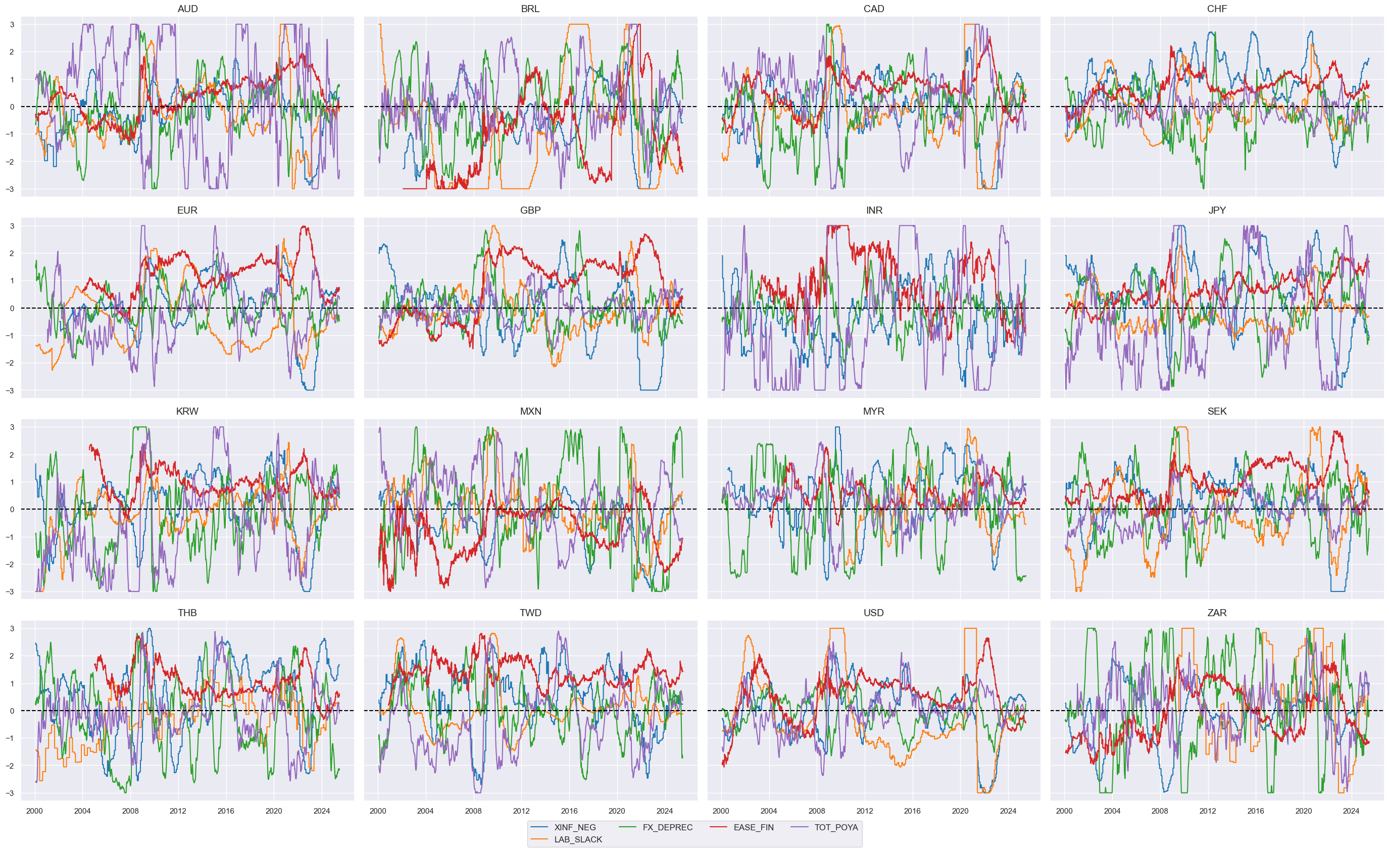
linear_composite
function is designed to calculate linear combinations of different categories. It can produce a composite even if some of the component data are missing. This flexibility is valuable because it enables to work with the available information rather than discarding it entirely. This behavior is desirable if one works with a composite of a set of categories that capture a similar underlying factor. In this context, the function calculates simple averages of the factors listed in
dict_factors
.
# Combine to thematic composite thematic scores

cidx = cids_eqxx
dfa = pd.DataFrame(columns=list(dfx.columns))

for key, value in dict_factors.items():
    xcatx = [x + "_ZN" for x in value]
    dfaa = msp.linear_composite(
        df=dfx,
        xcats=xcatx,
        cids=cidx,
        complete_xcats=False,
        new_xcat=key,
    )
    dfa = msm.update_df(dfa, dfaa)

dfx = msm.update_df(dfx, dfa)
cidx = cids_eqxx
xcatx = list(dict_factors.keys())

msp.view_timelines(
    dfx,
    xcats=xcatx,
    cids=cidx,
    ncol=4,
    start="2000-01-01",
    same_y=True,
)
# Re-score composites

cidx = cids_eqxx
xcatx = list(dict_factors.keys())

dfa = pd.DataFrame(columns=list(dfx.columns))

for xc in xcatx:
    dfaa = msp.make_zn_scores(
        dfx,
        xcat=xc,
        cids=cidx,
        sequential=True,
        min_obs=261 * 5,
        neutral="zero",
        pan_weight=1,  # assumes comparable impact scales across cross-sections
        thresh=3,
        postfix="_ZN",
        est_freq="m",
    )
    dfa = msm.update_df(dfa, dfaa)

dfx = msm.update_df(dfx, dfa)
themz = [x + "_ZN" for x in list(dict_factors.keys())]
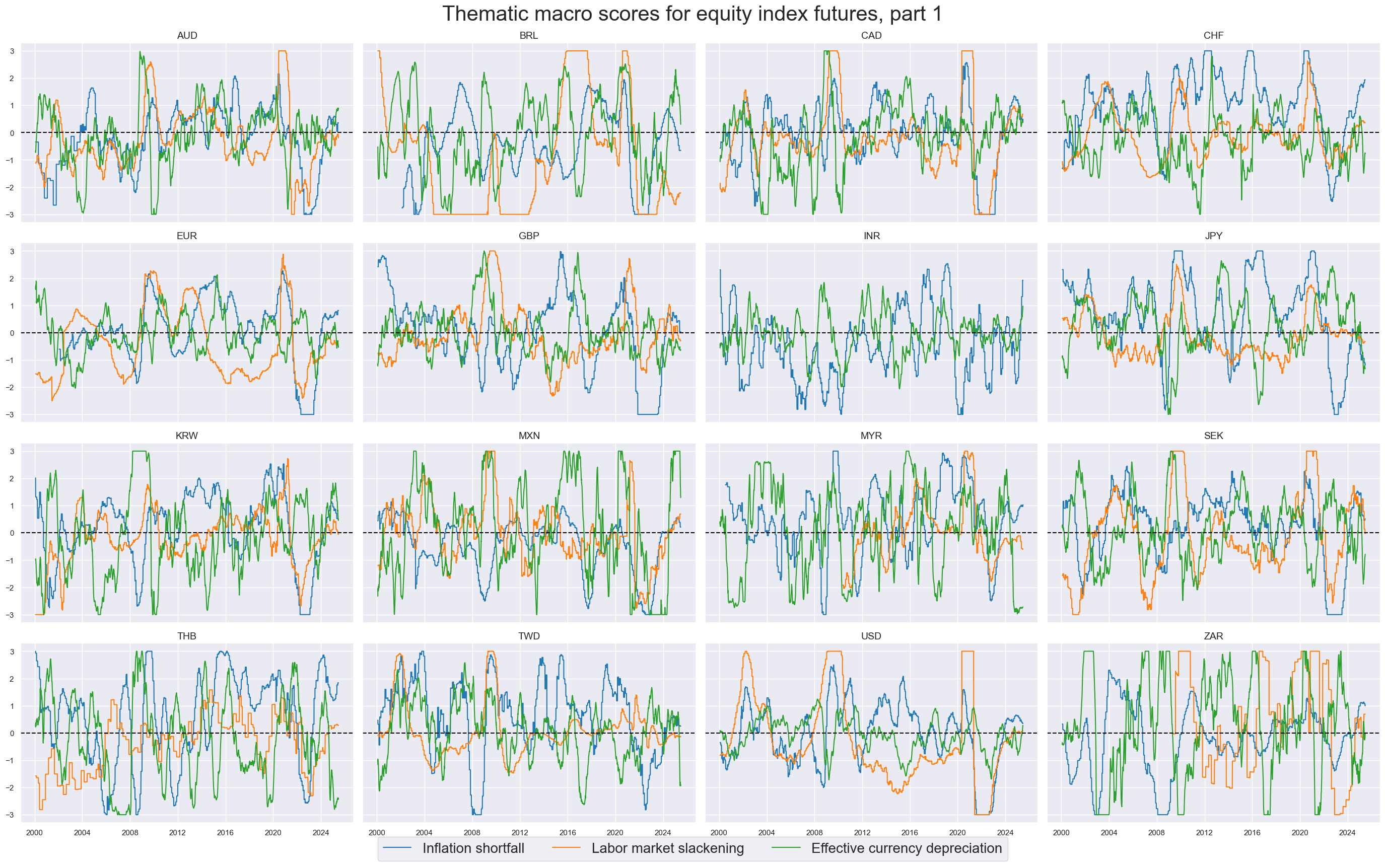
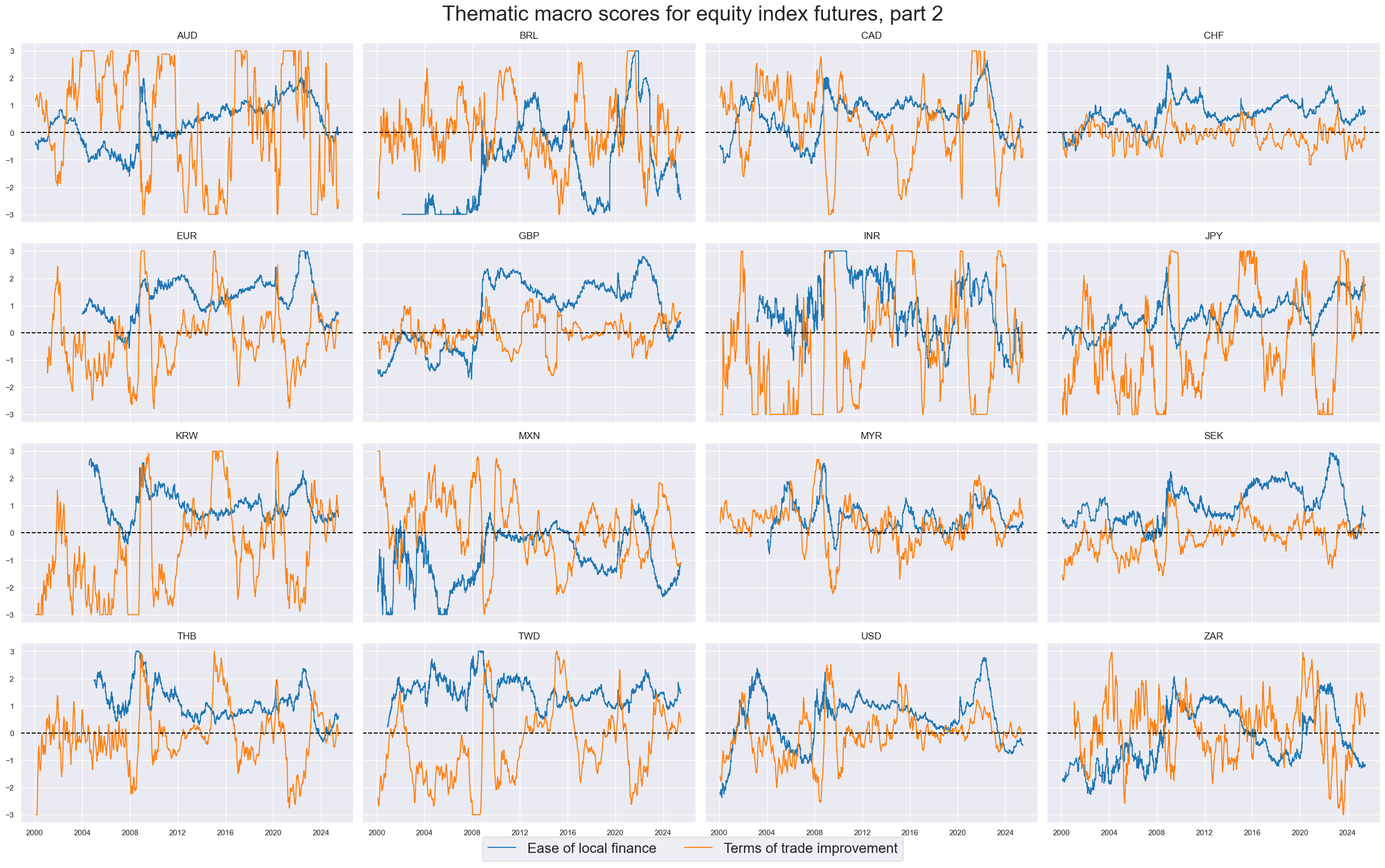
The below code defines a dictionary
dict_themes
with various macroeconomic themes and their descriptions, and then creates a list of the keys from this dictionary. This approach ensures that the labels associated with each theme are more readable and accessible.
# Labelling dictionary

dict_themes = {}
dict_themes["ALL_MACRO_ZN"] = "All macro themes"
dict_themes["XINF_NEG_ZN"] = "Inflation shortfall"
dict_themes["LAB_SLACK_ZN"] = "Labor market slackening"
dict_themes["FX_DEPREC_ZN"] = "Effective currency depreciation"
dict_themes["EASE_FIN_ZN"] = "Ease of local finance"
dict_themes["TOT_POYA_ZN"] = "Terms of trade improvement"

macroz = list(dict_themes.keys())
cidx = cids_eqxx
xcatx = themz[:3]

msp.view_timelines(
    dfx,
    xcats=xcatx,
    cids=cidx,
    title="Thematic macro scores for equity index futures, part 1",
    title_fontsize=30,
    xcat_labels=[dict_themes[xc] for xc in xcatx],
    legend_fontsize=20,
    ncol=4,
    start="2000-01-01",
    same_y=True,
)

xcatx = themz[3:]
msp.view_timelines(
    dfx,
    xcats=xcatx,
    cids=cidx,
    title="Thematic macro scores for equity index futures, part 2",
    title_fontsize=30,
    xcat_labels=[dict_themes[xc] for xc in xcatx],
    legend_fontsize=20,
    ncol=4,
    start="2000-01-01",
    same_y=True,
)
Grand total macro score #
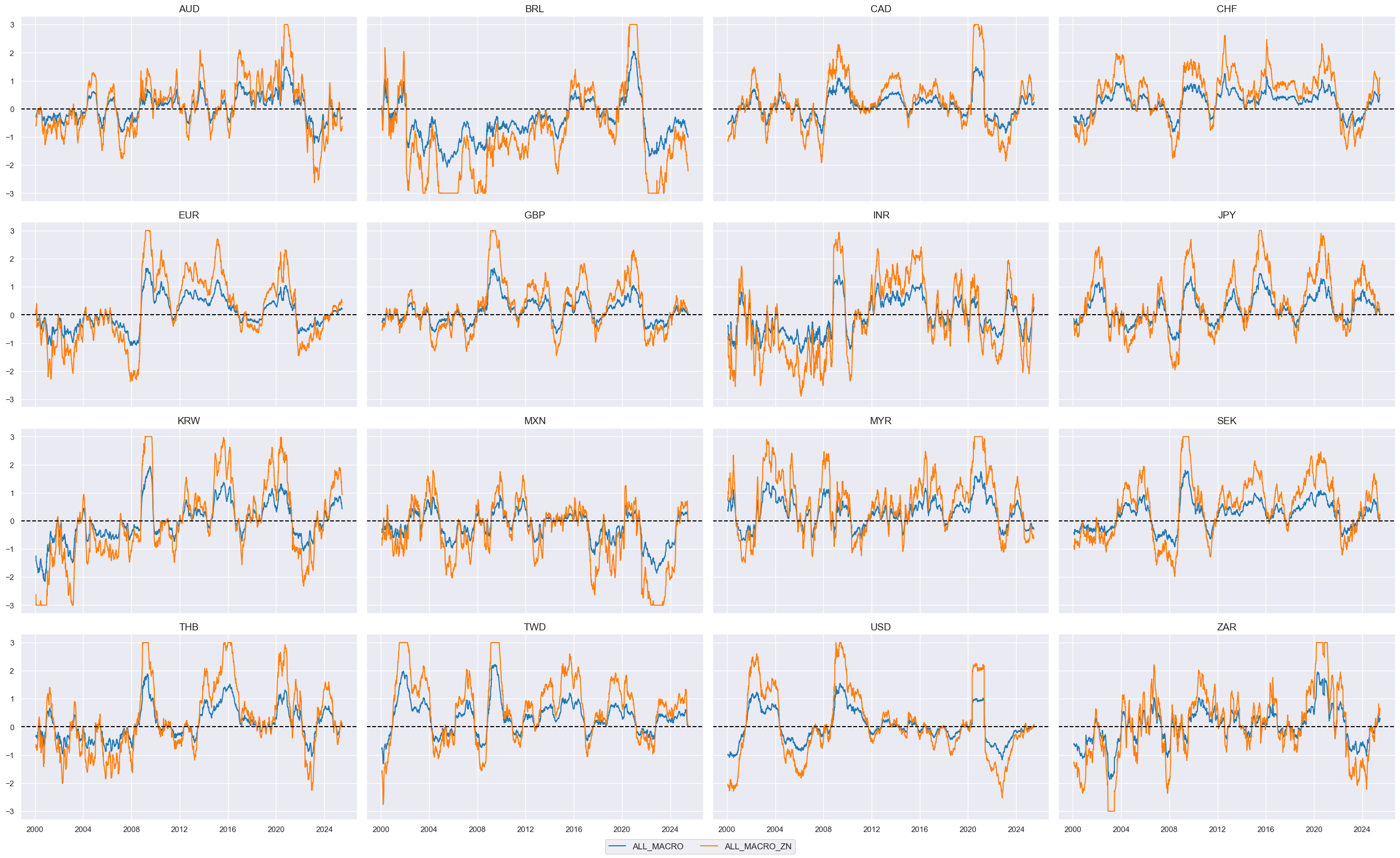
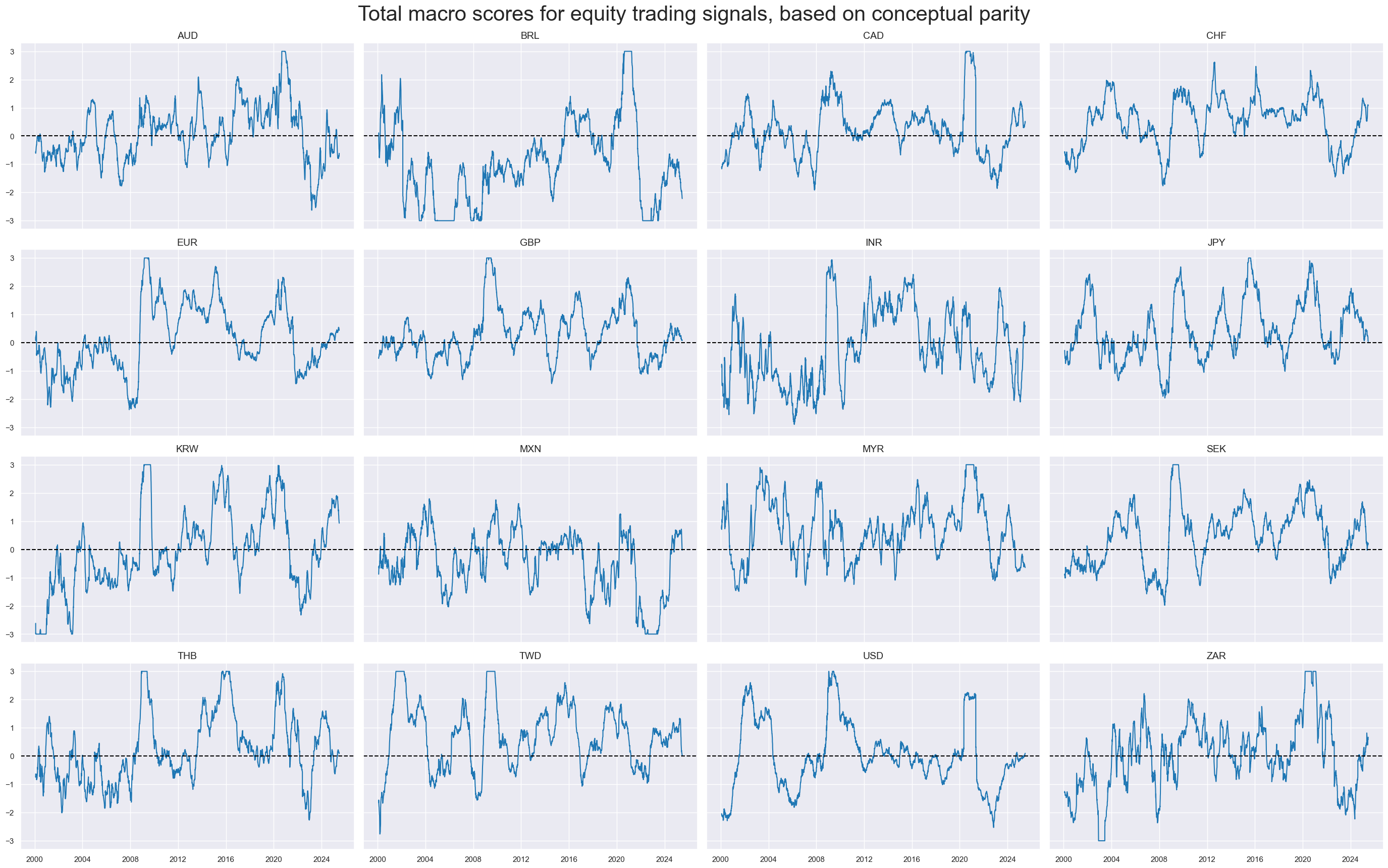
All five themes—Inflation shortfall, Labor market slackening, Effective currency depreciation, Ease of local finance, and Terms of trade improvement—are combined into a composite score using equal weights. This new indicator is standardized into a z-score and given the suffix
_ZN
, resulting in the label
ALL_MACRO_ZN
.There is no optimization involved.
# Combine to grand total

cidx = cids_eqxx
xcatx = themz

dfa = msp.linear_composite(
    df=dfx,
    xcats=xcatx,
    cids=cidx,
    complete_xcats=False,
    new_xcat="ALL_MACRO",
)
dfx = msm.update_df(dfx, dfa)

# Re-score

dfa = msp.make_zn_scores(
    dfx,
    xcat="ALL_MACRO",
    cids=cidx,
    sequential=True,
    min_obs=261 * 5,
    neutral="zero",
    pan_weight=1,  # assumes comparable impact scales across cross-sections
    thresh=3,
    postfix="_ZN",
    est_freq="m",
)
dfx = msm.update_df(dfx, dfa)

# Add to labelling dictionary

dict_themes["ALL_MACRO_ZN"] = "All macro themes" # updating dict_themes with the new indicator
cidx = cids_eqxx
xcatx = ["ALL_MACRO", "ALL_MACRO_ZN"]

msp.view_timelines(
    dfx,
    xcats=xcatx,
    cids=cidx,
    ncol=4,
    start="2000-01-01",
    same_y=True,
)
cidx = cids_eqxx
xcatx = ["ALL_MACRO_ZN"]

msp.view_timelines(
    dfx,
    xcats=xcatx,
    cids=cidx,
    title="Total macro scores for equity trading signals, based on conceptual parity",
    title_fontsize=30,
    xcat_labels=[dict_themes[xc] for xc in xcatx],
    legend_fontsize=20,
    ncol=4,
    start="2000-01-01",
    same_y=True,
)
Relative scores #
DM basket #
The convenience function
make_relative_value()
of the
macrosynergy.panel
module calculates values relative to an equally-weighted basket of developed market currencies, which are specified in the list
cids_dmeq
, while adapting to missing periods of any of the basket cross sections.
update_df()
function in the
macrosynergy
management module concatenates two JPMaQS data frames, effectively adding the newly calculated relative indicators with postfix
vDM
.
cidx = cids_dmeq
xcatx = macroz

dfa = msp.make_relative_value(
    dfx,
    xcats=xcatx,
    cids=cidx,
    start="2000-01-01",
    blacklist=fxblack,  # cross-sections can be blacklisted for calculation and basket use
    rel_meth="subtract",
    complete_cross=False,  # cross-sections do not have to be complete for basket calculation
    postfix="vDM",
)
dfx = msm.update_df(dfx, dfa)

macroz_vdm = [x + "vDM" for x in macroz]
macro = macroz[0]  # check composite score
cidx = cids_dmeq
xcatx = [macro, f"{macro}vDM"]

msp.view_timelines(
    dfx,
    xcats=xcatx,
    cids=cidx,
    ncol=4,
    start="2000-01-01",
    same_y=True,
)

Global basket #
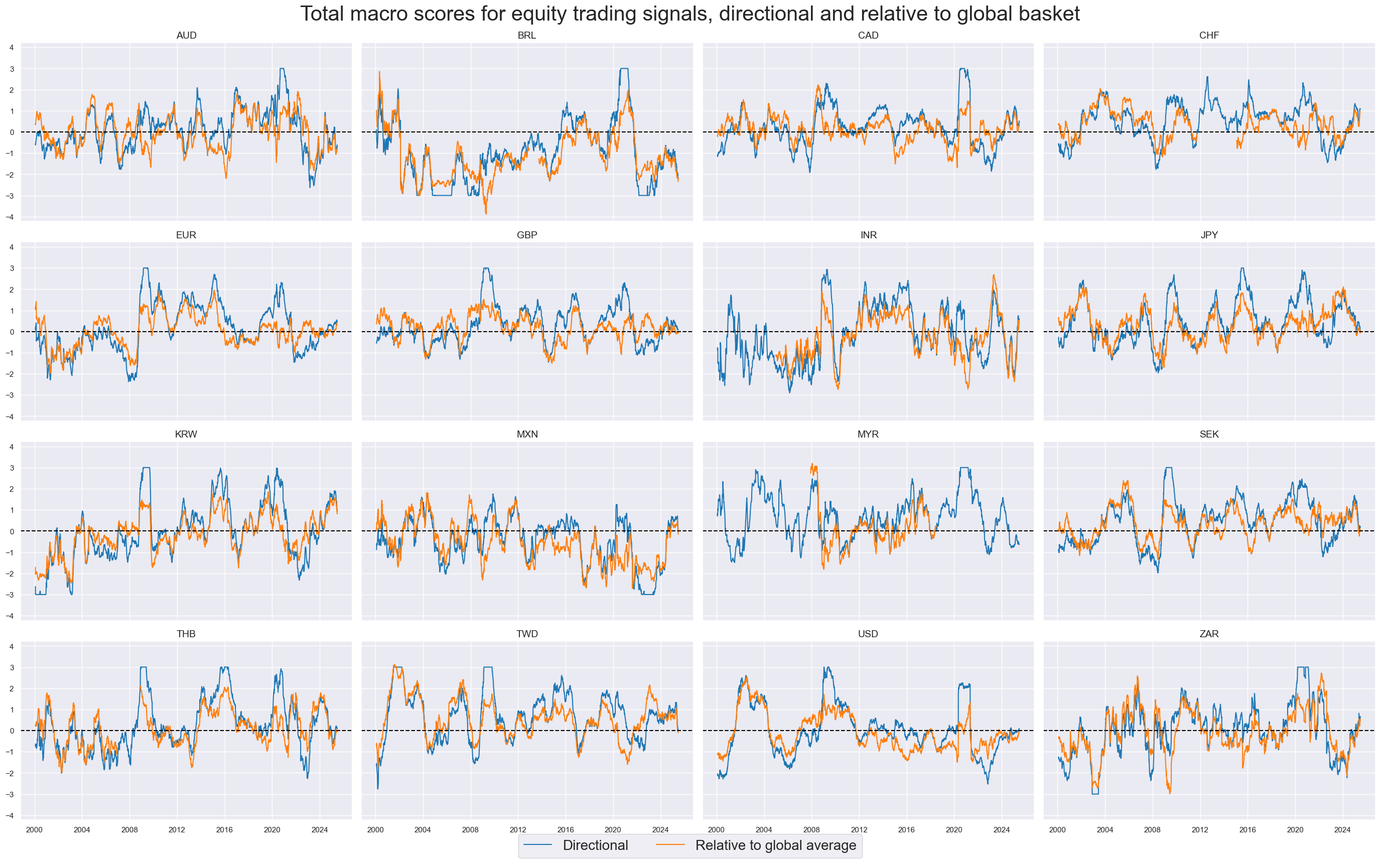
The
make_relative_value()
function from the
macrosynergy.panel
module calculates values relative to an equally-weighted basket of available market
cids_eqxx
. This basket includes all available market cross-sections and adapts to any missing periods within these cross-sections. The newly generated global relative indicators are then appended with the postfix
vGM
, differentiating them from the relative indicator calculated earlier.
cidx = cids_eqxx
xcatx = macroz

dfa = msp.make_relative_value(
    dfx,
    xcats=xcatx,
    cids=cidx,
    start="2000-01-01",
    blacklist=fxblack,  # cross-sections can be blacklisted for calculation and basket use
    rel_meth="subtract",
    complete_cross=False,  # cross-sections do not have to be complete for basket calculation
    postfix="vGM",
)
dfx = msm.update_df(dfx, dfa)

macroz_vgm = [x + "vGM" for x in macroz]
macro = macroz[0]  # pick a composite score
cidx = cids_eqxx
xcatx = [macro, f"{macro}vGM"]

msp.view_timelines(
    dfx,
    xcats=xcatx,
    cids=cidx,
    title="Total macro scores for equity trading signals, directional and relative to global basket",
    title_fontsize=30,
    xcat_labels=["Directional", "Relative to global average"],
    legend_fontsize=20,
    ncol=4,
    start="2000-01-01",
    same_y=True,
)
Target returns #
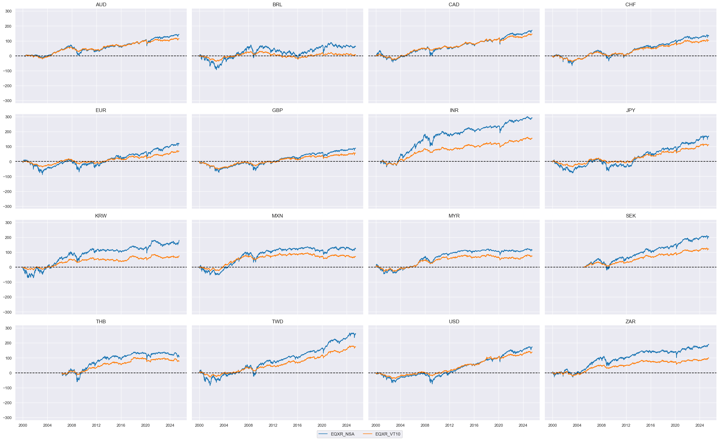
Outright equity index returns #
cidx = cids_eqxx
xcatx = ["EQXR_NSA", "EQXR_VT10"]

msp.view_timelines(
    dfx,
    xcats=xcatx,
    cids=cidx,
    ncol=4,
    start="2000-01-01",
    same_y=True,
    cumsum=True,
)
Relative equity index returns #
DM basket #
The code below calculates relative values for equity index futures relative to a basket of all available market currencies specified in the list
cids_dmeq
. The newly calculated relative indicators are assigned the suffix
vDM
.
cidx = cids_dmeq
xcatx = ["EQXR_NSA", "EQXR_VT10"]

dfa = msp.make_relative_value(
    dfx,
    xcats=xcatx,
    cids=cidx,
    start="2000-01-01",
    blacklist=fxblack,  # cross-sections can be blacklisted for calculation and basket use
    rel_meth="subtract",
    complete_cross=False,  # cross-sections do not have to be complete for basket calculation
    postfix="vDM",
)
dfx = msm.update_df(dfx, dfa)
cidx = cids_dmeq
xcatx = ["EQXR_NSAvDM", "EQXR_VT10vDM"]

msp.view_timelines(
    dfx,
    xcats=xcatx,
    cids=cidx,
    ncol=4,
    start="2000-01-01",
    same_y=True,
    cumsum=True,
)

Global basket #
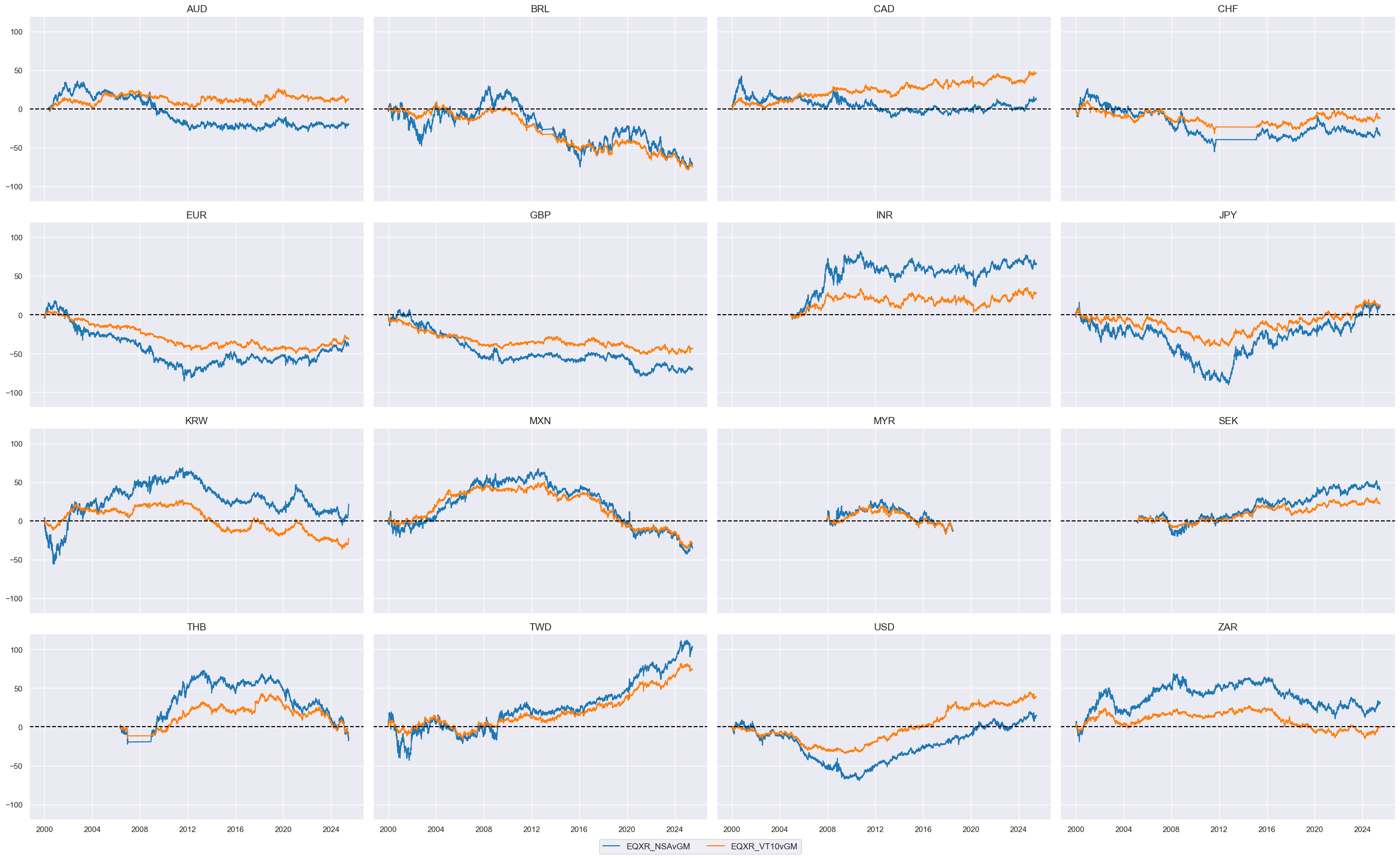
The code below calculates relative values for equity index futures relative to a basket of all available market currencies specified in the list
cids_eqxx
. The newly calculated relative indicators are assigned the suffix
vGM
.
cidx = cids_eqxx
xcatx = ["EQXR_NSA", "EQXR_VT10"]

dfa = msp.make_relative_value(
    dfx,
    xcats=xcatx,
    cids=cidx,
    start="2000-01-01",
    blacklist=fxblack,  # cross-sections can be blacklisted for calculation and basket use
    rel_meth="subtract",
    complete_cross=False,  # cross-sections do not have to be complete for basket calculation
    postfix="vGM",
)
dfx = msm.update_df(dfx, dfa)
cidx = cids_eqxx
xcatx = ["EQXR_NSAvGM", "EQXR_VT10vGM"]

msp.view_timelines(
    dfx,
    xcats=xcatx,
    cids=cidx,
    ncol=4,
    start="2000-01-01",
    same_y=True,
    cumsum=True,
)
Value checks #
Global directional futures strategy #
Specs and panel test #
We start by defining a dictionary with the key parameters necessary for evaluating a specific type of strategy. This includes setting the signals, target returns, cross-sections, initial date, and blacklistings for evaluating a global directional futures strategy.
dict_deq_gm = {
    "sigs": macroz,
    "targs": ["EQXR_NSA", "EQXR_VT10"],
    "cidx": cids_eqxx,
    "start": "2000-01-01",
    "black": fxblack,
    "srr": None,
    "pnls": None,
}
Instances of the
CategoryRelations
class from the
macrosynnergy.panel
package are designed to organize panels of features and targets into formats suitable for analysis. This class provides functionalities for frequency conversion, adding lags, and trimming outliers.
dix = dict_deq_gm

sig = dix["sigs"][0]
targ = dix["targs"][1]
blax = dix["black"]
cidx = dix["cidx"]
start = dix["start"]

cr = msp.CategoryRelations(
    dfx,
    xcats=[sig, targ],
    cids=cidx,
    freq="Q",
    lag=1,
    xcat_aggs=["last", "sum"],
    start=start,
    blacklist=blax,
)
cr.reg_scatter(
    labels=False,
    coef_box="lower left",
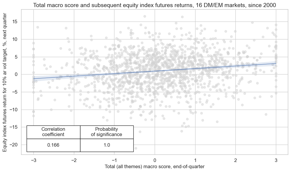
    title="Total macro score and subsequent equity index futures returns, 16 DM/EM markets, since 2000",
    xlab="Total (all themes) macro score, end-of-quarter",
    ylab="Equity index futures return for 10% ar vol target, %, next quarter",
    size=(10, 6),
    prob_est="map",
)
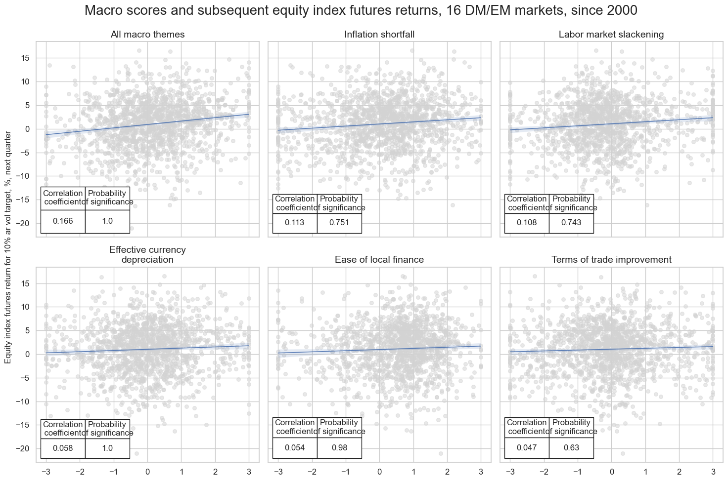
multiple_reg_scatter()
method allows comparison of several pairs of two categories relationships side by side, including the strength of the linear association and any potential outliers.
dix = dict_deq_gm

sigs = dix["sigs"]
targ = dix["targs"][1] # assuming just one target
blax = dix["black"]
cidx = dix["cidx"]
start = dix["start"]

# Initialize the dictionary to store CategoryRelations instances

dict_cr = {}

for sig in sigs:
    dict_cr[sig] = msp.CategoryRelations(
        dfx,
        xcats=[sig, targ],
        cids=cidx,
        freq="Q",
        lag=1,
        xcat_aggs=["last", "sum"],
        start=start,
        blacklist=blax,
    )

# Plotting the results

crs = list(dict_cr.values())
crs_keys = list(dict_cr.keys())

msv.multiple_reg_scatter(
    cat_rels=crs,
    title="Macro scores and subsequent equity index futures returns, 16 DM/EM markets, since 2000",
    ylab="Equity index futures return for 10% ar vol target, %, next quarter",
    ncol=3,
    nrow=2,
    figsize=(15, 10),
    prob_est="map",
    coef_box="lower left",
    subplot_titles=[dict_themes[k] for k in crs_keys],
)
LAB_SLACK_ZN misses: ['INR'].
Accuracy and correlation check #
Please refer to the
SignalReturnRelations
class of the
macrosynergy.signal
module for details on the code below.
dix = dict_deq_gm

sigx = dix["sigs"]
targx = dix["targs"]
cidx = dix["cidx"]
start = dix["start"]
blax = dix["black"]

srr = mss.SignalReturnRelations(
    dfx,
    cids=cidx,
    sigs=sigx,
    rets=targx,
    freqs="M",
    start=start,
    blacklist=blax,
)

dix["srr"] = srr
dix = dict_deq_gm
srr = dix["srr"]
display(srr.multiple_relations_table().astype("float").round(3))
| accuracy | bal_accuracy | pos_sigr | pos_retr | pos_prec | neg_prec | pearson | pearson_pval | kendall | kendall_pval | auc | ||||
|---|---|---|---|---|---|---|---|---|---|---|---|---|---|---|
| Return | Signal | Frequency | Aggregation | |||||||||||
| EQXR_NSA | ALL_MACRO_ZN | M | last | 0.539 | 0.531 | 0.548 | 0.585 | 0.613 | 0.449 | 0.125 | 0.000 | 0.067 | 0.000 | 0.532 |
| EASE_FIN_ZN | M | last | 0.558 | 0.522 | 0.727 | 0.589 | 0.602 | 0.443 | 0.041 | 0.007 | 0.035 | 0.001 | 0.518 | |
| FX_DEPREC_ZN | M | last | 0.515 | 0.516 | 0.491 | 0.585 | 0.602 | 0.431 | 0.042 | 0.006 | 0.028 | 0.005 | 0.517 | |
| LAB_SLACK_ZN | M | last | 0.481 | 0.499 | 0.397 | 0.586 | 0.585 | 0.413 | 0.075 | 0.000 | 0.033 | 0.002 | 0.499 | |
| TOT_POYA_ZN | M | last | 0.510 | 0.514 | 0.476 | 0.585 | 0.600 | 0.428 | 0.052 | 0.000 | 0.020 | 0.046 | 0.515 | |
| XINF_NEG_ZN | M | last | 0.535 | 0.524 | 0.569 | 0.587 | 0.607 | 0.440 | 0.083 | 0.000 | 0.040 | 0.000 | 0.524 | |
| EQXR_VT10 | ALL_MACRO_ZN | M | last | 0.539 | 0.531 | 0.548 | 0.585 | 0.614 | 0.449 | 0.102 | 0.000 | 0.061 | 0.000 | 0.532 |
| EASE_FIN_ZN | M | last | 0.558 | 0.522 | 0.727 | 0.590 | 0.602 | 0.443 | 0.029 | 0.059 | 0.025 | 0.014 | 0.518 | |
| FX_DEPREC_ZN | M | last | 0.515 | 0.516 | 0.491 | 0.585 | 0.602 | 0.431 | 0.025 | 0.092 | 0.019 | 0.053 | 0.517 | |
| LAB_SLACK_ZN | M | last | 0.482 | 0.499 | 0.397 | 0.586 | 0.586 | 0.413 | 0.063 | 0.000 | 0.028 | 0.008 | 0.499 | |
| TOT_POYA_ZN | M | last | 0.510 | 0.514 | 0.476 | 0.586 | 0.600 | 0.428 | 0.036 | 0.015 | 0.017 | 0.082 | 0.515 | |
| XINF_NEG_ZN | M | last | 0.535 | 0.524 | 0.569 | 0.587 | 0.608 | 0.440 | 0.079 | 0.000 | 0.040 | 0.000 | 0.524 |
Naive PnL #
The
NaivePnL
class of the
macrosynergy.pnl
module is the basis for calculating simple stylized PnLs for various signals under consideration of correlation benchmarks.
dix = dict_deq_gm

sigx = dix["sigs"]
targ = dix["targs"][1]
cidx = dix["cidx"]
blax = dix["black"]
start = dix["start"]

naive_pnl = msn.NaivePnL(
    dfx,
    ret=targ,
    sigs=sigx,
    cids=cidx,
    start=start,
    blacklist=blax,
    bms=["USD_EQXR_NSA"],
)

for sig in sigx:
    naive_pnl.make_pnl(
        sig,
        sig_neg=False,
        sig_op="raw",
        sig_add=0,
        thresh=3,
        rebal_freq="monthly",
        vol_scale=10,
        rebal_slip=1,
        pnl_name=sig+"_RAW"
    )

for sig in sigx[:2]:
    naive_pnl.make_pnl(
        sig,
        sig_neg=False,
        sig_op="raw",
        sig_add=1,
        thresh=3,
        rebal_freq="monthly",
        vol_scale=10,
        rebal_slip=1,
        pnl_name=sig+"_RAWLB1"
    )

naive_pnl.make_long_pnl(vol_scale=10, label="Long only")

dix["pnls"] = naive_pnl
dix = dict_deq_gm

start = dix["start"]
cidx = dix["cidx"]
sigx = [dix["sigs"][0]]

naive_pnl = dix["pnls"]
vers = ["_RAW", "_RAWLB1"]
pnls = [s + v for s in sigx for v in vers] + ["Long only"]

desc = [
    "based on total macro score (no long bias)",
    "based on total macro score, with long bias (1 standard deviation)",
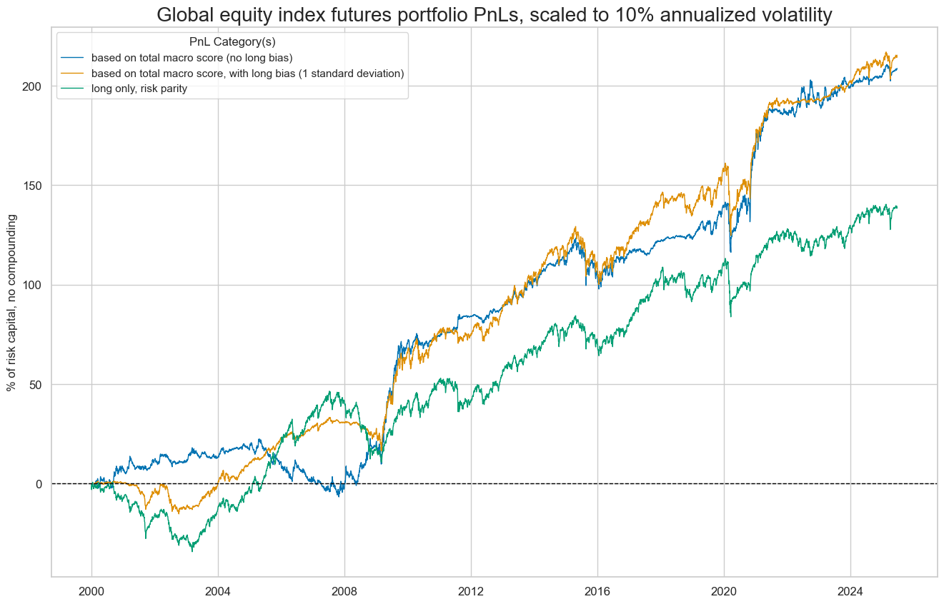
    "long only, risk parity",

]

labels = {key: desc for key, desc in zip(pnls, desc)}

naive_pnl.plot_pnls(
    pnl_cats=pnls,
    pnl_cids=["ALL"],
    start=start,
    title="Global equity index futures portfolio PnLs, scaled to 10% annualized volatility",
    xcat_labels=labels,
    figsize=(16, 10),
)
dix = dict_deq_gm

start = dix["start"]
cidx = dix["cidx"]
sigx = dix["sigs"][2:]

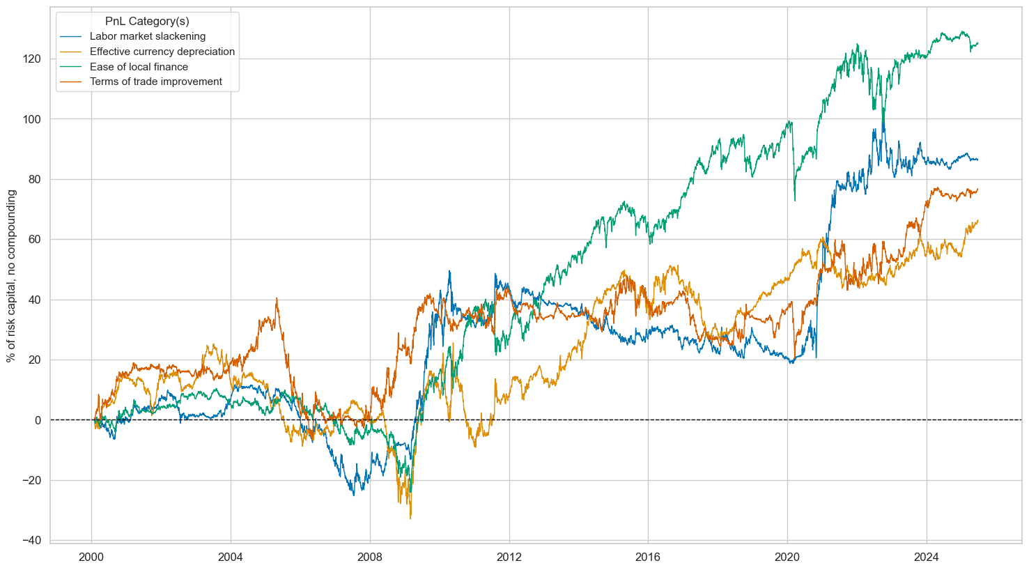
lab={key + "_RAW": value for key, value in dict_themes.items()}
labels = dict(list(lab.items())[2:])

naive_pnl = dix["pnls"]
pnls = [s + "_RAW" for s in sigx]

naive_pnl.plot_pnls(
    pnl_cats=pnls,
    pnl_cids=["ALL"],
    start=start,
    title=None,
    xcat_labels=labels,
    figsize=(18, 10),
)
dix = dict_deq_gm
start = dix["start"]
sigx = dix["sigs"]
naive_pnl = dix["pnls"]

pnls = [sig + "_RAW" for sig in sigx] + ["ALL_MACRO_ZN_RAWLB1", "Long only"]

df_eval = naive_pnl.evaluate_pnls(
    pnl_cats=pnls,
    pnl_cids=["ALL"],
    start=start,
)

labels={key + "_RAW": value for key, value in dict_themes.items()}
labels['ALL_MACRO_ZN_RAWLB1'] = 'All macro, long bias (1std)'

df_eval = df_eval.rename(columns=labels)

display(df_eval.transpose().astype("float").round(3))
| Return % | St. Dev. % | Sharpe Ratio | Sortino Ratio | Max 21-Day Draw % | Max 6-Month Draw % | Peak to Trough Draw % | Top 5% Monthly PnL Share | USD_EQXR_NSA correl | Traded Months | |
|---|---|---|---|---|---|---|---|---|---|---|
| xcat | ||||||||||
| All macro themes | 8.223 | 10.0 | 0.822 | 1.202 | -24.175 | -18.663 | -29.119 | 0.694 | 0.101 | 306.0 |
| Inflation shortfall | 5.958 | 10.0 | 0.596 | 0.862 | -20.435 | -24.336 | -35.807 | 0.935 | -0.083 | 306.0 |
| Labor market slackening | 3.412 | 10.0 | 0.341 | 0.507 | -17.899 | -16.335 | -36.911 | 1.613 | -0.116 | 306.0 |
| Effective currency depreciation | 2.589 | 10.0 | 0.259 | 0.376 | -16.152 | -28.833 | -58.225 | 1.685 | 0.071 | 306.0 |
| Ease of local finance | 4.936 | 10.0 | 0.494 | 0.685 | -25.234 | -22.649 | -34.623 | 0.908 | 0.339 | 306.0 |
| Terms of trade improvement | 3.025 | 10.0 | 0.302 | 0.443 | -18.763 | -30.351 | -46.999 | 1.642 | 0.035 | 306.0 |
| All macro, long bias (1std) | 8.483 | 10.0 | 0.848 | 1.178 | -33.402 | -22.560 | -36.395 | 0.533 | 0.478 | 306.0 |
| Long only | 5.474 | 10.0 | 0.547 | 0.743 | -26.587 | -26.748 | -35.676 | 0.622 | 0.595 | 306.0 |
DM directional futures strategy #
This section deals with the same global directional futures strategy as above, but just for developed markets.
Specs and panel test #
dict_deq_dm = {
    "sigs": macroz,
    "targs": ["EQXR_NSA", "EQXR_VT10"],
    "cidx": cids_dmeq,
    "start": "2000-01-01",
    "black": fxblack,
    "srr": None,
    "pnls": None,
}
dix = dict_deq_dm

sig = dix["sigs"][0]
targ = dix["targs"][1]
blax = dix["black"]
cidx = dix["cidx"]
start = dix["start"]

cr = msp.CategoryRelations(
    dfx,
    xcats=[sig, targ],
    cids=cidx,
    freq="Q",
    lag=1,
    xcat_aggs=["last", "sum"],
    start=start,
    blacklist=blax,
)
cr.reg_scatter(
    labels=False,
    coef_box="lower left",
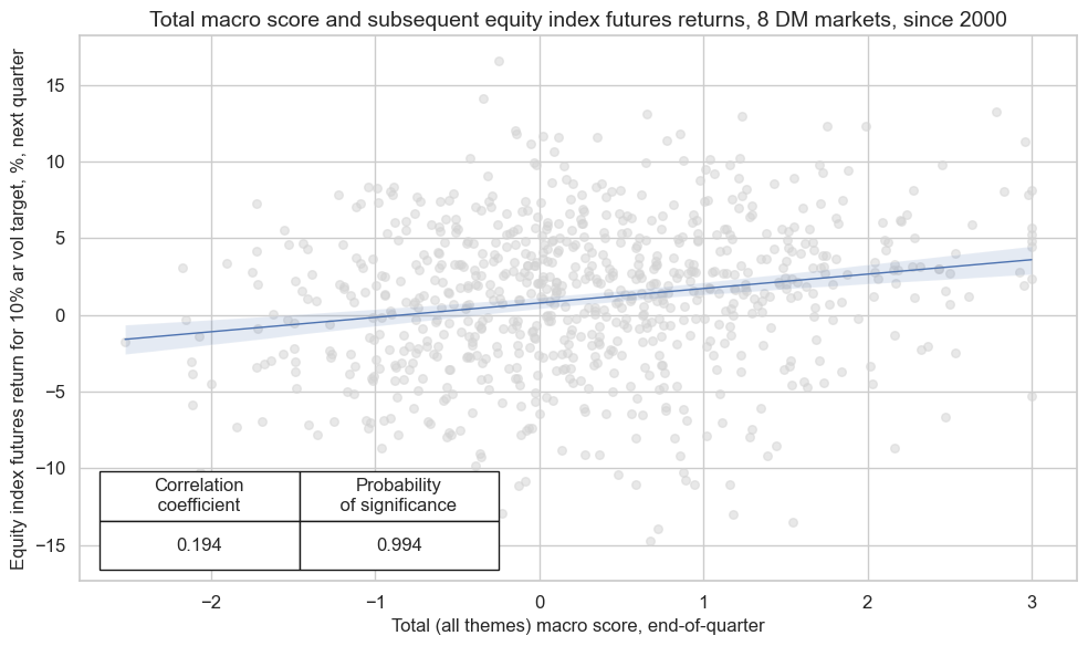
    title="Total macro score and subsequent equity index futures returns, 8 DM markets, since 2000",
    xlab="Total (all themes) macro score, end-of-quarter",
    ylab="Equity index futures return for 10% ar vol target, %, next quarter",
    size=(10, 6),
    prob_est="map",
)
dix = dict_deq_dm

sigs = dix["sigs"]
targ = dix["targs"][1]
blax = dix["black"]
cidx = dix["cidx"]
start = dix["start"]

# Initialize the dictionary to store CategoryRelations instances

dict_cr = {}

for sig in sigs:
    dict_cr[sig] = msp.CategoryRelations(
        dfx,
        xcats=[sig, targ],
        cids=cidx,
        freq="Q",
        lag=1,
        xcat_aggs=["last", "sum"],
        start=start,
        blacklist=blax,
    )

# Plotting the results

crs = list(dict_cr.values())
crs_keys = list(dict_cr.keys())

msv.multiple_reg_scatter(
    cat_rels=crs,
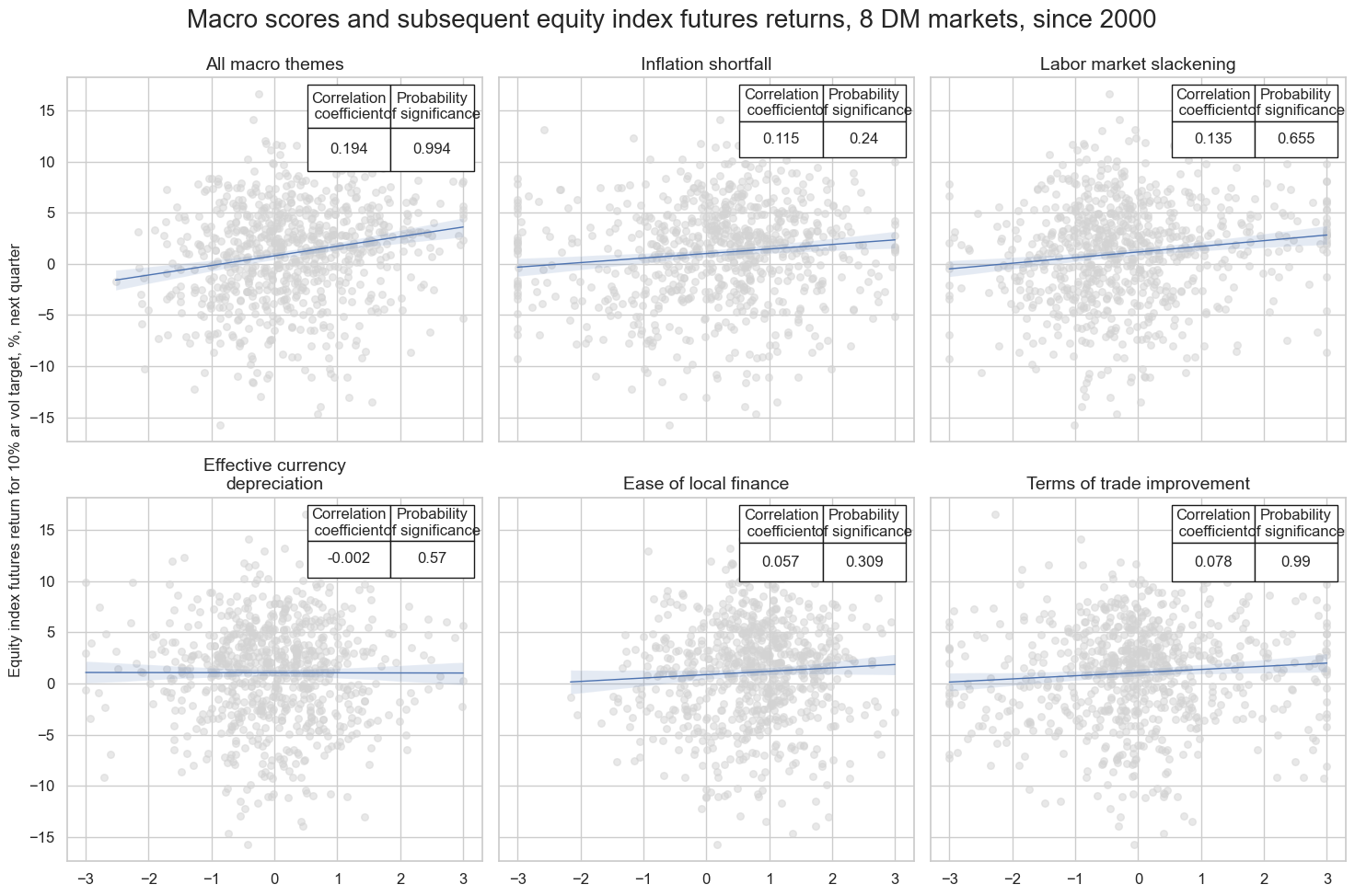
    title="Macro scores and subsequent equity index futures returns, 8 DM markets, since 2000",
    ylab="Equity index futures return for 10% ar vol target, %, next quarter",
    ncol=3,
    nrow=2,
    figsize=(15, 10),
    prob_est="map",
    coef_box="upper right",
    subplot_titles=[dict_themes[k] for k in crs_keys],
)
Accuracy and correlation check #
dix = dict_deq_dm

sigx = dix["sigs"]
targx = dix["targs"]
cidx = dix["cidx"]
start = dix["start"]
blax = dix["black"]

srr = mss.SignalReturnRelations(
    dfx,
    cids=cidx,
    sigs=sigx,
    rets=targx,
    freqs="M",
    start=start,
    blacklist=blax,
)

dix["srr"] = srr
dix = dict_deq_dm

srr = dix["srr"]

display(srr.multiple_relations_table().astype("float").round(3))
| accuracy | bal_accuracy | pos_sigr | pos_retr | pos_prec | neg_prec | pearson | pearson_pval | kendall | kendall_pval | auc | ||||
|---|---|---|---|---|---|---|---|---|---|---|---|---|---|---|
| Return | Signal | Frequency | Aggregation | |||||||||||
| EQXR_NSA | ALL_MACRO_ZN | M | last | 0.555 | 0.539 | 0.586 | 0.602 | 0.634 | 0.443 | 0.140 | 0.000 | 0.081 | 0.000 | 0.539 |
| EASE_FIN_ZN | M | last | 0.585 | 0.534 | 0.801 | 0.605 | 0.618 | 0.450 | 0.049 | 0.018 | 0.033 | 0.017 | 0.523 | |
| FX_DEPREC_ZN | M | last | 0.494 | 0.497 | 0.483 | 0.602 | 0.599 | 0.395 | 0.005 | 0.799 | -0.002 | 0.858 | 0.497 | |
| LAB_SLACK_ZN | M | last | 0.476 | 0.504 | 0.363 | 0.602 | 0.607 | 0.401 | 0.081 | 0.000 | 0.044 | 0.001 | 0.504 | |
| TOT_POYA_ZN | M | last | 0.522 | 0.526 | 0.480 | 0.603 | 0.629 | 0.422 | 0.054 | 0.009 | 0.036 | 0.010 | 0.527 | |
| XINF_NEG_ZN | M | last | 0.562 | 0.539 | 0.622 | 0.604 | 0.634 | 0.445 | 0.098 | 0.000 | 0.061 | 0.000 | 0.539 | |
| EQXR_VT10 | ALL_MACRO_ZN | M | last | 0.555 | 0.539 | 0.586 | 0.602 | 0.635 | 0.443 | 0.116 | 0.000 | 0.067 | 0.000 | 0.539 |
| EASE_FIN_ZN | M | last | 0.585 | 0.534 | 0.801 | 0.605 | 0.619 | 0.450 | 0.023 | 0.264 | 0.013 | 0.362 | 0.523 | |
| FX_DEPREC_ZN | M | last | 0.494 | 0.498 | 0.483 | 0.602 | 0.600 | 0.395 | -0.003 | 0.891 | -0.002 | 0.912 | 0.498 | |
| LAB_SLACK_ZN | M | last | 0.476 | 0.505 | 0.363 | 0.602 | 0.608 | 0.401 | 0.070 | 0.001 | 0.032 | 0.019 | 0.505 | |
| TOT_POYA_ZN | M | last | 0.521 | 0.525 | 0.480 | 0.603 | 0.629 | 0.421 | 0.056 | 0.007 | 0.034 | 0.015 | 0.526 | |
| XINF_NEG_ZN | M | last | 0.563 | 0.540 | 0.622 | 0.604 | 0.634 | 0.445 | 0.080 | 0.000 | 0.050 | 0.000 | 0.539 |
Naive PnL #
dix = dict_deq_dm

sigx = dix["sigs"]
targ = dix["targs"][1]
cidx = dix["cidx"]
blax = dix["black"]
start = dix["start"]

naive_pnl = msn.NaivePnL(
    dfx,
    ret=targ,
    sigs=sigx,
    cids=cidx,
    start=start,
    blacklist=blax,
    bms=["USD_EQXR_NSA"],
)

for sig in sigx:
    naive_pnl.make_pnl(
        sig,
        sig_neg=False,
        sig_op="raw",
        sig_add=0,
        thresh=3,
        rebal_freq="monthly",
        vol_scale=10,
        rebal_slip=1,
        pnl_name=sig+"_RAW"
    )

for sig in sigx[:2]:
    naive_pnl.make_pnl(
        sig,
        sig_neg=False,
        sig_op="raw",
        sig_add=1, # long bias, 1 standard deviation
        thresh=3,
        rebal_freq="monthly",
        vol_scale=10,
        rebal_slip=1,
        pnl_name=sig+"_RAWLB1"
    )

naive_pnl.make_long_pnl(vol_scale=10, label="Long only")

dix["pnls"] = naive_pnl
dix = dict_deq_dm

start = dix["start"]
cidx = dix["cidx"]
sigx = [dix["sigs"][0]]

naive_pnl = dix["pnls"]
vers = ["_RAW", "_RAWLB1"]
pnls = [s + v for s in sigx for v in vers] + ["Long only"]

desc = [
    "based on total macro score (no long bias)",
    "based on total macro score, with long bias (1 standard deviation)",
    "long only, risk parity",

]

labels = {key: desc for key, desc in zip(pnls, desc)}


naive_pnl.plot_pnls(
    pnl_cats=pnls,
    pnl_cids=["ALL"],
    start=start,
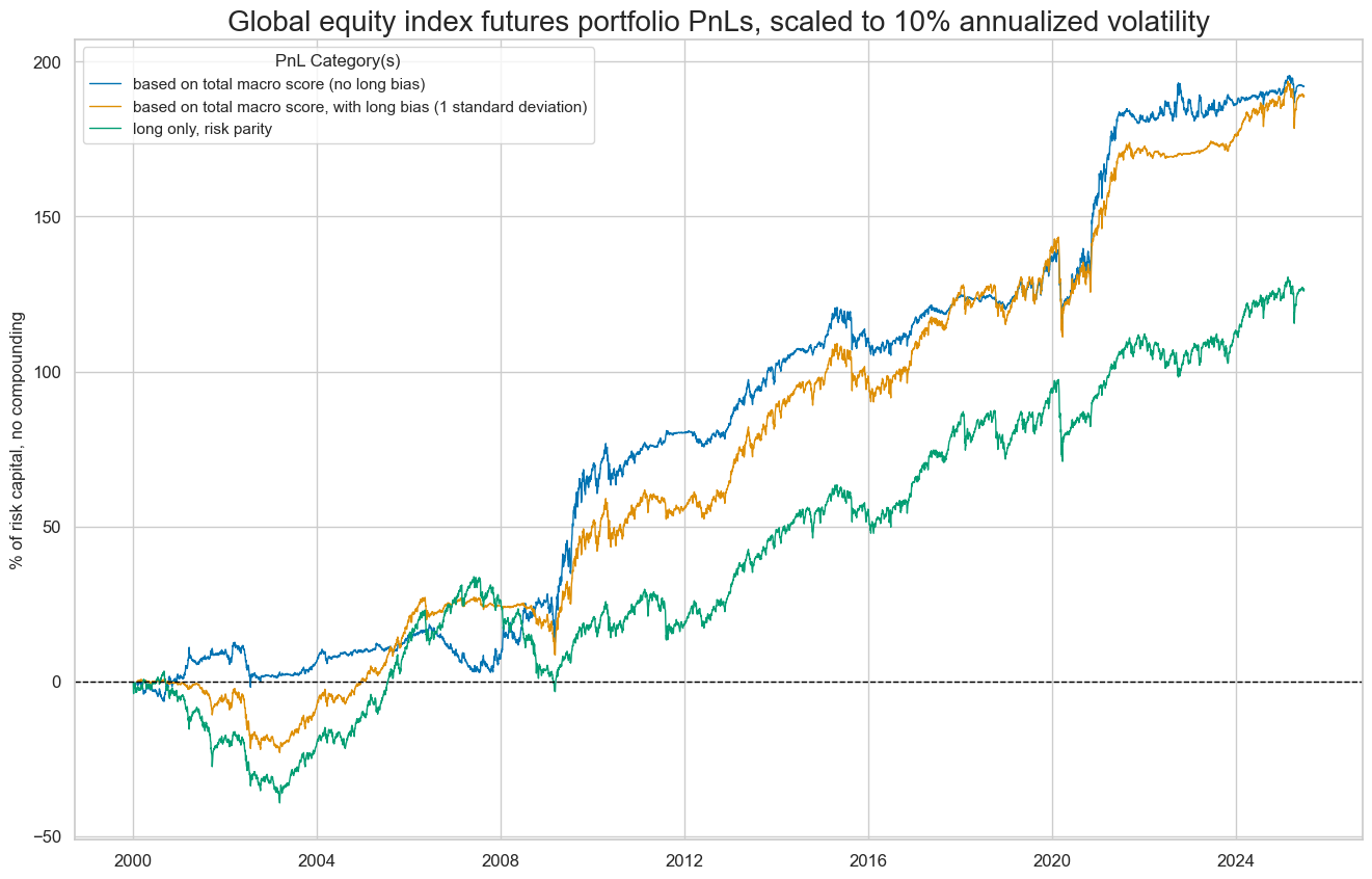
    title="Global equity index futures portfolio PnLs, scaled to 10% annualized volatility",
    xcat_labels=labels,
    figsize=(16, 10),
)
dix = dict_deq_dm

start = dix["start"]
cidx = dix["cidx"]
sigx = dix["sigs"][2:]

naive_pnl = dix["pnls"]
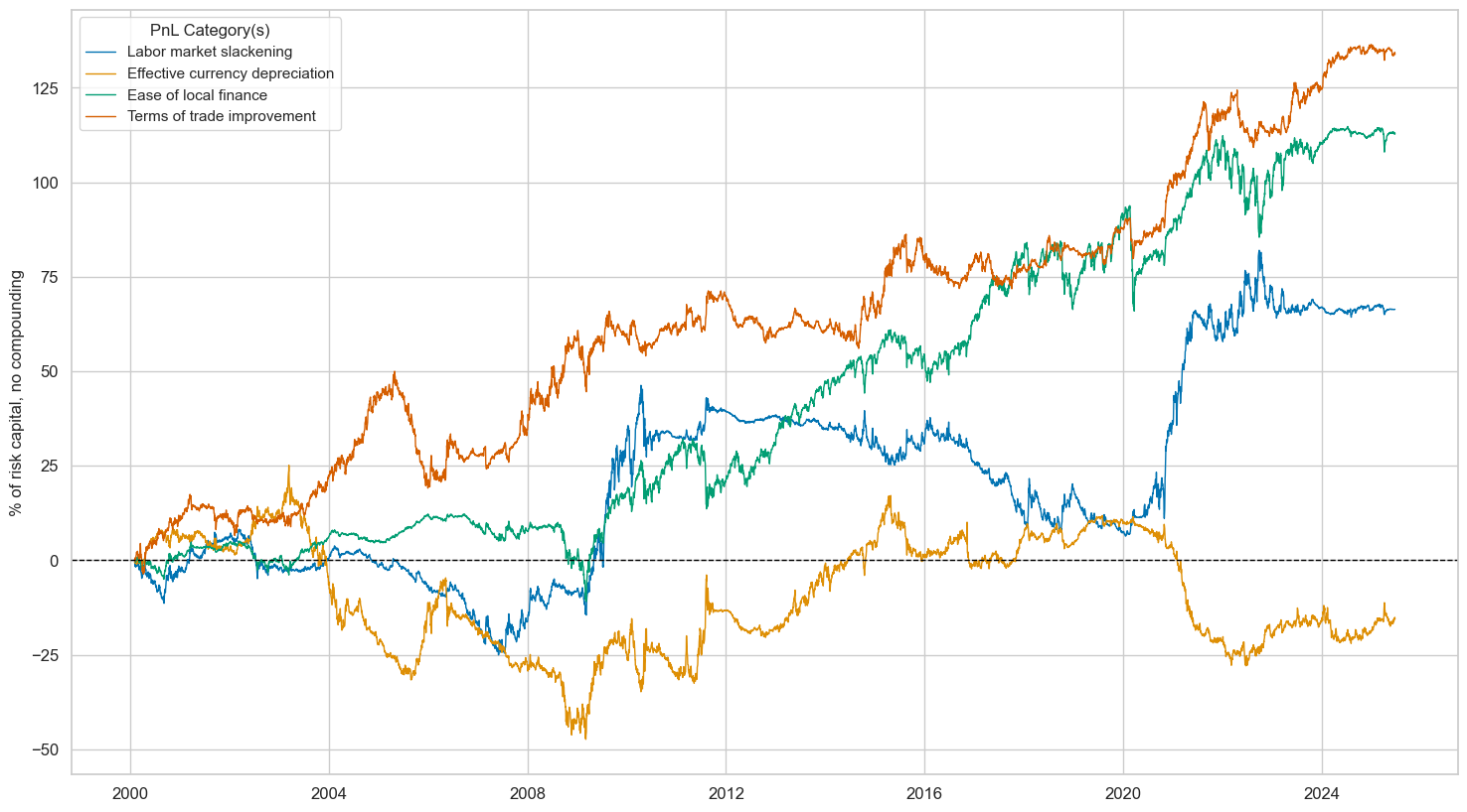
pnls = [s + "_RAW" for s in sigx]

lab={key + "_RAW": value for key, value in dict_themes.items()}
labels = dict(list(lab.items())[2:])

naive_pnl.plot_pnls(
    pnl_cats=pnls,
    pnl_cids=["ALL"],
    start=start,
    title=None,
    xcat_labels=labels,
    figsize=(18, 10),
)
dix = dict_deq_dm
start = dix["start"]
sigx = dix["sigs"]
naive_pnl = dix["pnls"]

pnls = [sig + "_RAW" for sig in sigx] + ["ALL_MACRO_ZN_RAWLB1", "Long only"]

df_eval = naive_pnl.evaluate_pnls(
    pnl_cats=pnls,
    pnl_cids=["ALL"],
    start=start,
)

labels={key + "_RAW": value for key, value in dict_themes.items()}
labels['ALL_MACRO_ZN_RAWLB1'] = 'All macro, long bias (1std)'

df_eval = df_eval.rename(columns=labels)

display(df_eval.transpose().astype("float").round(3))
| Return % | St. Dev. % | Sharpe Ratio | Sortino Ratio | Max 21-Day Draw % | Max 6-Month Draw % | Peak to Trough Draw % | Top 5% Monthly PnL Share | USD_EQXR_NSA correl | Traded Months | |
|---|---|---|---|---|---|---|---|---|---|---|
| xcat | ||||||||||
| All macro themes | 7.567 | 10.0 | 0.757 | 1.101 | -24.126 | -14.257 | -24.866 | 0.695 | 0.227 | 306.0 |
| Inflation shortfall | 4.992 | 10.0 | 0.499 | 0.714 | -17.763 | -25.500 | -35.777 | 0.967 | 0.011 | 306.0 |
| Labor market slackening | 2.615 | 10.0 | 0.261 | 0.389 | -17.875 | -14.930 | -39.879 | 1.995 | -0.075 | 306.0 |
| Effective currency depreciation | -0.615 | 10.0 | -0.061 | -0.087 | -12.758 | -24.289 | -72.524 | -5.593 | 0.001 | 306.0 |
| Ease of local finance | 4.451 | 10.0 | 0.445 | 0.612 | -26.924 | -21.755 | -27.867 | 0.858 | 0.504 | 306.0 |
| Terms of trade improvement | 5.269 | 10.0 | 0.527 | 0.776 | -12.152 | -24.221 | -30.921 | 0.808 | 0.003 | 306.0 |
| All macro, long bias (1std) | 7.450 | 10.0 | 0.745 | 1.037 | -31.202 | -18.680 | -32.247 | 0.550 | 0.542 | 306.0 |
| Long only | 4.973 | 10.0 | 0.497 | 0.677 | -25.526 | -21.066 | -42.577 | 0.644 | 0.630 | 306.0 |
dix = dict_deq_dm
cidx = dix["cidx"]
sig = dix["sigs"][0]
start = dix["start"]

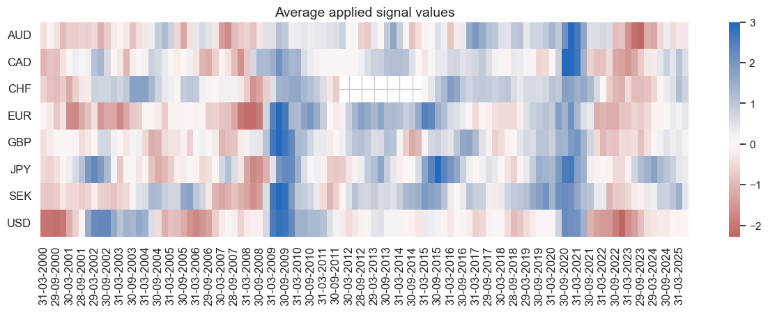
naive_pnl.signal_heatmap(
    pnl_name=sig + "_RAW",
    pnl_cids=cidx,
    freq="q",
    start=start,
    figsize=(15, 4),
)
Global relative futures strategy #
This section examines global relative value signals.
Specs and panel test #
dict_req_gm = {
    "sigs": macroz_vgm,
    "targs": ["EQXR_VT10vGM"],
    "cidx": cids_eqxx,
    "start": "2000-01-01",
    "black": fxblack,
    "srr": None,
    "pnls": None,
}

# For labelling
dict_themes_vgm = {
    key + "vGM": value + " (relative)" for key, value in dict_themes.items()
}
dix = dict_req_gm

sigs = dix["sigs"]
targ = dix["targs"][0]
blax = dix["black"]
cidx = dix["cidx"]
start = dix["start"]

# Initialize the dictionary to store CategoryRelations instances

dict_cr = {}

for sig in sigs:
    dict_cr[sig] = msp.CategoryRelations(
        dfx,
        xcats=[sig, targ],
        cids=cidx,
        freq="Q",
        lag=1,
        xcat_aggs=["last", "sum"],
        start=start,
        blacklist=blax,
    )

# Plotting the results

crs = list(dict_cr.values())
crs_keys = list(dict_cr.keys())

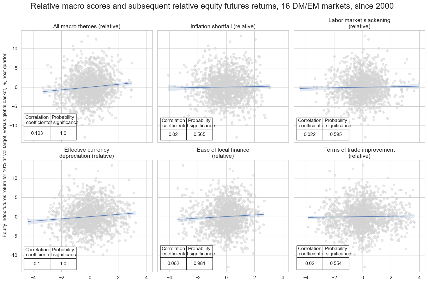
msv.multiple_reg_scatter(
    cat_rels=crs,
    title="Relative macro scores and subsequent relative equity futures returns, 16 DM/EM markets, since 2000",
    ylab="Equity index futures return for 10% ar vol target, versus global basket, %, next quarter",
    ncol=3,
    nrow=2,
    figsize=(15, 10),
    prob_est="map",
    coef_box="lower left",
    subplot_titles=[dict_themes_vgm[k] for k in crs_keys],
)
LAB_SLACK_ZNvGM misses: ['INR'].
Accuracy and correlation check #
dix = dict_req_gm

sigx = dix["sigs"]
targx = dix["targs"]
cidx = dix["cidx"]
start = dix["start"]
blax = dix["black"]

srr = mss.SignalReturnRelations(
    dfx,
    cids=cidx,
    sigs=sigx,
    rets=targx,
    freqs="M",
    start=start,
    blacklist=blax,
)

dix["srr"] = srr
dix = dict_req_gm
srr = dix["srr"]

display(srr.multiple_relations_table().astype("float").round(3))
| accuracy | bal_accuracy | pos_sigr | pos_retr | pos_prec | neg_prec | pearson | pearson_pval | kendall | kendall_pval | auc | ||||
|---|---|---|---|---|---|---|---|---|---|---|---|---|---|---|
| Return | Signal | Frequency | Aggregation | |||||||||||
| EQXR_VT10vGM | ALL_MACRO_ZNvGM | M | last | 0.510 | 0.510 | 0.513 | 0.493 | 0.504 | 0.517 | 0.061 | 0.000 | 0.032 | 0.001 | 0.510 |
| EASE_FIN_ZNvGM | M | last | 0.519 | 0.520 | 0.551 | 0.494 | 0.512 | 0.528 | 0.038 | 0.012 | 0.025 | 0.013 | 0.520 | |
| FX_DEPREC_ZNvGM | M | last | 0.518 | 0.518 | 0.499 | 0.493 | 0.512 | 0.525 | 0.053 | 0.000 | 0.029 | 0.004 | 0.518 | |
| LAB_SLACK_ZNvGM | M | last | 0.500 | 0.500 | 0.521 | 0.492 | 0.492 | 0.508 | 0.004 | 0.788 | 0.003 | 0.786 | 0.500 | |
| TOT_POYA_ZNvGM | M | last | 0.514 | 0.514 | 0.506 | 0.494 | 0.508 | 0.521 | 0.023 | 0.127 | 0.017 | 0.094 | 0.514 | |
| XINF_NEG_ZNvGM | M | last | 0.510 | 0.510 | 0.503 | 0.494 | 0.504 | 0.516 | 0.008 | 0.576 | 0.001 | 0.917 | 0.510 |
Naive PnL #
dix = dict_req_gm

sigx = dix["sigs"]
targ = dix["targs"][0]
cidx = dix["cidx"]
blax = dix["black"]
start = dix["start"]

naive_pnl = msn.NaivePnL(
    dfx,
    ret=targ,
    sigs=sigx,
    cids=cidx,
    start=start,
    blacklist=blax,
    bms=["USD_EQXR_NSA"],
)

for sig in sigx:
    naive_pnl.make_pnl(
        sig,
        sig_neg=False,
        sig_op="raw",
        sig_add=0,
        thresh=3,
        rebal_freq="monthly",
        vol_scale=10,
        rebal_slip=1,
        pnl_name=sig+"_RAW"
    )


dix["pnls"] = naive_pnl
dix = dict_req_gm

start = dix["start"]
cidx = dix["cidx"]
sig = dix["sigs"][0]

naive_pnl = dix["pnls"]
pnls = [sig + "_RAW"]


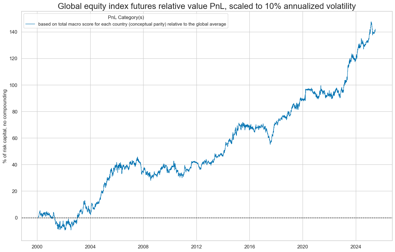
naive_pnl.plot_pnls(
    pnl_cats=pnls,
    pnl_cids=["ALL"],
    start=start,
    title="Global equity index futures relative value PnL, scaled to 10% annualized volatility",
    xcat_labels=["based on total macro score for each country (conceptual parity) relative to the global average"],
    figsize=(16, 10),
)
dix = dict_req_gm

start = dix["start"]
cidx = dix["cidx"]
sigx = dix["sigs"][1:]

naive_pnl = dix["pnls"]
pnls = [s + "_RAW" for s in sigx]

lab={key + "_RAW": value for key, value in dict_themes_vgm.items()}
labels = dict(list(lab.items())[1:])

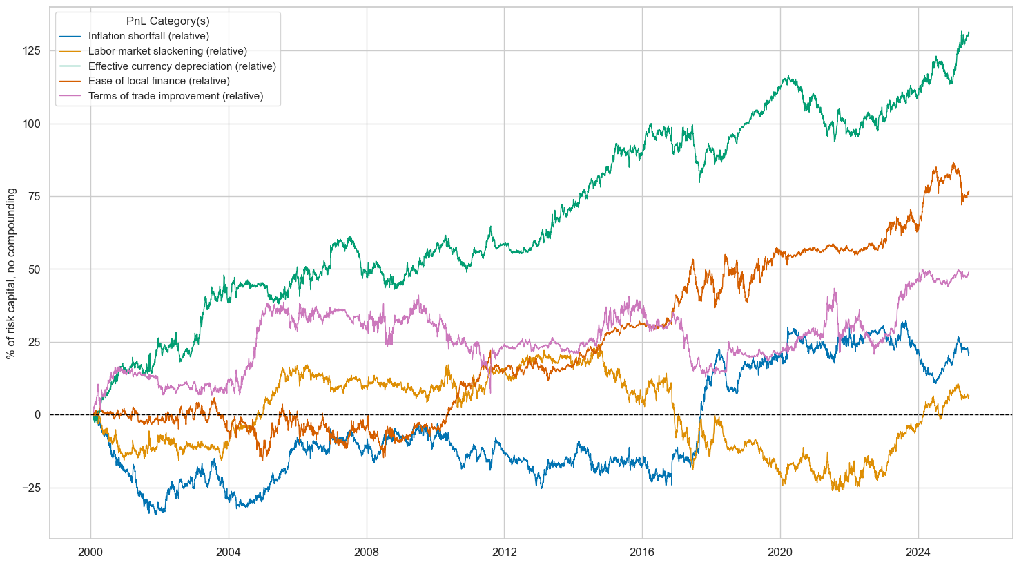
naive_pnl.plot_pnls(
    pnl_cats=pnls,
    pnl_cids=["ALL"],
    start=start,
    title=None,
    xcat_labels=labels,
    figsize=(18, 10),
)
dix = dict_req_gm
start = dix["start"]
sigx = dix["sigs"]

naive_pnl = dix["pnls"]
pnls = [sig + "_RAW" for sig in sigx]

labels={key + "_RAW": value for key, value in dict_themes_vgm.items()}


df_eval = naive_pnl.evaluate_pnls(
    pnl_cats=pnls,
    pnl_cids=["ALL"],
    start=start,
)
df_eval = df_eval.rename(columns=labels)

display(df_eval.transpose().astype("float").round(3))
| Return % | St. Dev. % | Sharpe Ratio | Sortino Ratio | Max 21-Day Draw % | Max 6-Month Draw % | Peak to Trough Draw % | Top 5% Monthly PnL Share | USD_EQXR_NSA correl | Traded Months | |
|---|---|---|---|---|---|---|---|---|---|---|
| xcat | ||||||||||
| All macro themes (relative) | 5.593 | 10.0 | 0.559 | 0.803 | -7.798 | -12.208 | -17.781 | 0.701 | -0.077 | 306.0 |
| Inflation shortfall (relative) | 0.849 | 10.0 | 0.085 | 0.123 | -8.866 | -15.772 | -34.905 | 4.324 | -0.083 | 306.0 |
| Labor market slackening (relative) | 0.259 | 10.0 | 0.026 | 0.037 | -11.985 | -22.702 | -50.538 | 11.025 | -0.058 | 306.0 |
| Effective currency depreciation (relative) | 5.154 | 10.0 | 0.515 | 0.747 | -9.973 | -18.865 | -22.669 | 0.639 | -0.016 | 306.0 |
| Ease of local finance (relative) | 3.032 | 10.0 | 0.303 | 0.427 | -11.609 | -13.537 | -21.591 | 1.114 | -0.134 | 306.0 |
| Terms of trade improvement (relative) | 1.937 | 10.0 | 0.194 | 0.278 | -20.503 | -17.901 | -33.728 | 1.979 | 0.104 | 306.0 |
DM relative futures strategy #
Relative equity futures strategy for developed markets
Specs and panel test #
dict_req_dm = {
    "sigs": macroz_vdm,
    "targs": ["EQXR_VT10vDM"],
    "cidx": cids_dmeq,
    "start": "2000-01-01",
    "black": fxblack,
    "srr": None,
    "pnls": None,
}

# For labelling
dict_themes_vdm = {
    key + "vDM": value + " (relative)" for key, value in dict_themes.items()
}
dix = dict_req_dm

sigs = dix["sigs"]
targ = dix["targs"][0]
blax = dix["black"]
cidx = dix["cidx"]
start = dix["start"]

# Initialize the dictionary to store CategoryRelations instances

dict_cr = {}

for sig in sigs:
    dict_cr[sig] = msp.CategoryRelations(
        dfx,
        xcats=[sig, targ],
        cids=cidx,
        freq="Q",
        lag=1,
        xcat_aggs=["last", "sum"],
        start=start,
        blacklist=blax,
    )

# Plotting the results

crs = list(dict_cr.values())
crs_keys = list(dict_cr.keys())

msv.multiple_reg_scatter(
    cat_rels=crs,
    title="Macro scores and subsequent equity index futures returns, 16 DM/EM markets, since 2000",
    ylab="Equity index futures return for 10% ar vol target, versus global basket, %, next quarter",
    ncol=3,
    nrow=2,
    figsize=(15, 10),
    prob_est="map",
    coef_box="lower left",
    subplot_titles=[dict_themes_vdm[k] for k in crs_keys],
)
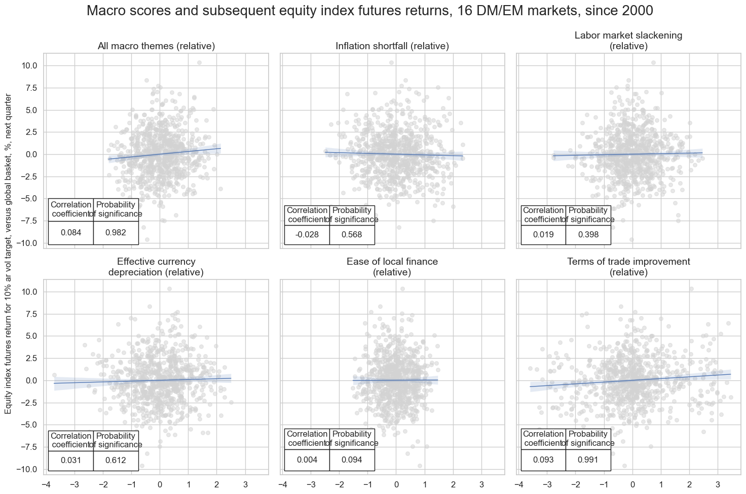
Accuracy and correlation check #
dix = dict_req_dm

sigx = dix["sigs"]
targx = dix["targs"]
cidx = dix["cidx"]
start = dix["start"]
blax = dix["black"]

srr = mss.SignalReturnRelations(
    dfx,
    cids=cidx,
    sigs=sigx,
    rets=targx,
    freqs="M",
    start=start,
    blacklist=blax,
)

dix["srr"] = srr
dix = dict_req_dm
srr = dix["srr"]

display(srr.multiple_relations_table().astype("float").round(3))
| accuracy | bal_accuracy | pos_sigr | pos_retr | pos_prec | neg_prec | pearson | pearson_pval | kendall | kendall_pval | auc | ||||
|---|---|---|---|---|---|---|---|---|---|---|---|---|---|---|
| Return | Signal | Frequency | Aggregation | |||||||||||
| EQXR_VT10vDM | ALL_MACRO_ZNvDM | M | last | 0.507 | 0.507 | 0.501 | 0.498 | 0.505 | 0.509 | 0.048 | 0.021 | 0.024 | 0.086 | 0.507 |
| EASE_FIN_ZNvDM | M | last | 0.514 | 0.514 | 0.500 | 0.500 | 0.514 | 0.515 | 0.005 | 0.817 | 0.009 | 0.525 | 0.514 | |
| FX_DEPREC_ZNvDM | M | last | 0.501 | 0.501 | 0.503 | 0.498 | 0.499 | 0.503 | 0.010 | 0.619 | 0.004 | 0.787 | 0.501 | |
| LAB_SLACK_ZNvDM | M | last | 0.506 | 0.506 | 0.484 | 0.498 | 0.504 | 0.508 | 0.000 | 0.989 | 0.003 | 0.820 | 0.506 | |
| TOT_POYA_ZNvDM | M | last | 0.511 | 0.511 | 0.484 | 0.498 | 0.509 | 0.512 | 0.063 | 0.002 | 0.035 | 0.012 | 0.511 | |
| XINF_NEG_ZNvDM | M | last | 0.497 | 0.497 | 0.484 | 0.498 | 0.495 | 0.498 | -0.016 | 0.444 | -0.013 | 0.354 | 0.497 |
Naive PnL #
dix = dict_req_dm

sigx = dix["sigs"]
targ = dix["targs"][0]
cidx = dix["cidx"]
blax = dix["black"]
start = dix["start"]

naive_pnl = msn.NaivePnL(
    dfx,
    ret=targ,
    sigs=sigx,
    cids=cidx,
    start=start,
    blacklist=blax,
    bms=["USD_EQXR_NSA"],
)

for sig in sigx:
    naive_pnl.make_pnl(
        sig,
        sig_neg=False,
        sig_op="raw",
        sig_add=0,
        thresh=3,
        rebal_freq="monthly",
        vol_scale=10,
        rebal_slip=1,
        pnl_name=sig+"_RAW"
    )


dix["pnls"] = naive_pnl
dix = dict_req_dm

start = dix["start"]
cidx = dix["cidx"]
sig = dix["sigs"][0]

naive_pnl = dix["pnls"]
pnls = [sig + "_RAW"]

naive_pnl.plot_pnls(
    pnl_cats=pnls,
    pnl_cids=["ALL"],
    start=start,
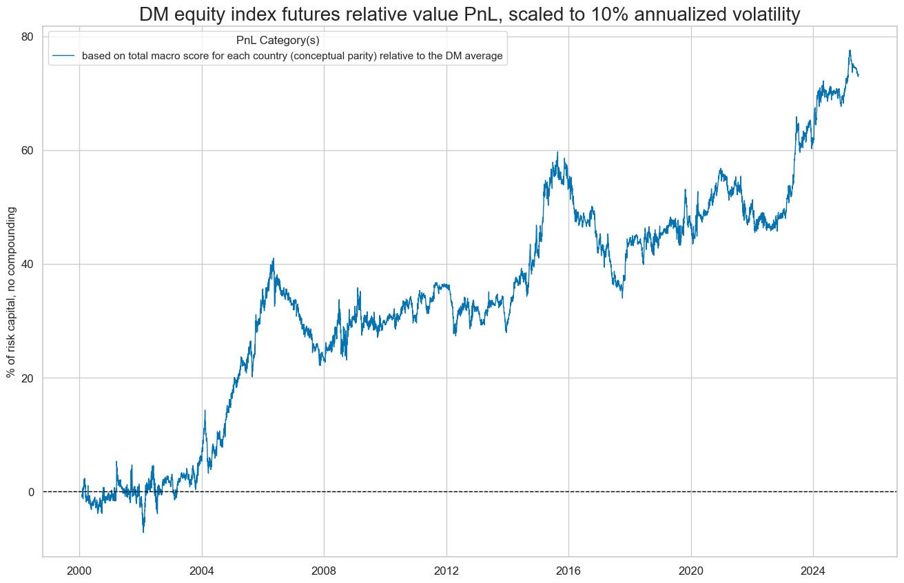
    title="DM equity index futures relative value PnL, scaled to 10% annualized volatility",
    xcat_labels=["based on total macro score for each country (conceptual parity) relative to the DM average"],
    figsize=(16, 10),
)
dix = dict_req_dm

start = dix["start"]
cidx = dix["cidx"]
sigx = dix["sigs"][1:]

naive_pnl = dix["pnls"]
pnls = [s + "_RAW" for s in sigx]


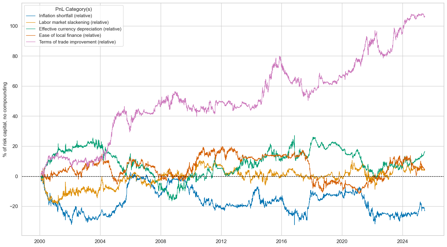
lab={key + "_RAW": value for key, value in dict_themes_vdm.items()}
labels = dict(list(lab.items())[1:])


naive_pnl.plot_pnls(
    pnl_cats=pnls,
    pnl_cids=["ALL"],
    start=start,
    title=None,
    xcat_labels=labels,
    figsize=(18, 10),
)
dix = dict_req_dm
start = dix["start"]
sigx = dix["sigs"]

naive_pnl = dix["pnls"]
pnls = [sig + "_RAW" for sig in sigx]

df_eval = naive_pnl.evaluate_pnls(
    pnl_cats=pnls,
    pnl_cids=["ALL"],
    start=start,
)

labels={key + "_RAW": value for key, value in dict_themes_vdm.items()}
df_eval = df_eval.rename(columns=labels)

display(df_eval.transpose().astype("float").round(3))
| Return % | St. Dev. % | Sharpe Ratio | Sortino Ratio | Max 21-Day Draw % | Max 6-Month Draw % | Peak to Trough Draw % | Top 5% Monthly PnL Share | USD_EQXR_NSA correl | Traded Months | |
|---|---|---|---|---|---|---|---|---|---|---|
| xcat | ||||||||||
| All macro themes (relative) | 2.882 | 10.0 | 0.288 | 0.417 | -9.039 | -11.619 | -25.778 | 1.103 | -0.079 | 306.0 |
| Inflation shortfall (relative) | -0.895 | 10.0 | -0.090 | -0.126 | -9.849 | -18.142 | -35.073 | -3.317 | -0.115 | 306.0 |
| Labor market slackening (relative) | 0.161 | 10.0 | 0.016 | 0.023 | -9.622 | -15.519 | -19.461 | 15.971 | 0.012 | 306.0 |
| Effective currency depreciation (relative) | 0.652 | 10.0 | 0.065 | 0.092 | -15.005 | -12.384 | -42.051 | 4.455 | -0.015 | 306.0 |
| Ease of local finance (relative) | 0.173 | 10.0 | 0.017 | 0.024 | -10.343 | -20.043 | -31.661 | 14.881 | 0.043 | 306.0 |
| Terms of trade improvement (relative) | 4.178 | 10.0 | 0.418 | 0.607 | -12.027 | -16.210 | -29.712 | 0.923 | -0.030 | 306.0 |