Emerging market macro risk scores

This category group comprises macro risk scores that reflect point-in-time states of economic indicators. The construction of these scores follows the methodology outlined in Macrosynergy’s research post here , which demonstrates how macro scores can be used to build macro risk premia indicators. These indicators, in turn, can serve as signals for fixed-income strategies. The research also explores the relationship between these signals and market returns—specifically foreign-currency bond index returns—highlighting a positive and statistically significant correlation. Selected results from the research are presented in this notebook.

Macro scores

Ticker : GFINRISK_NSA

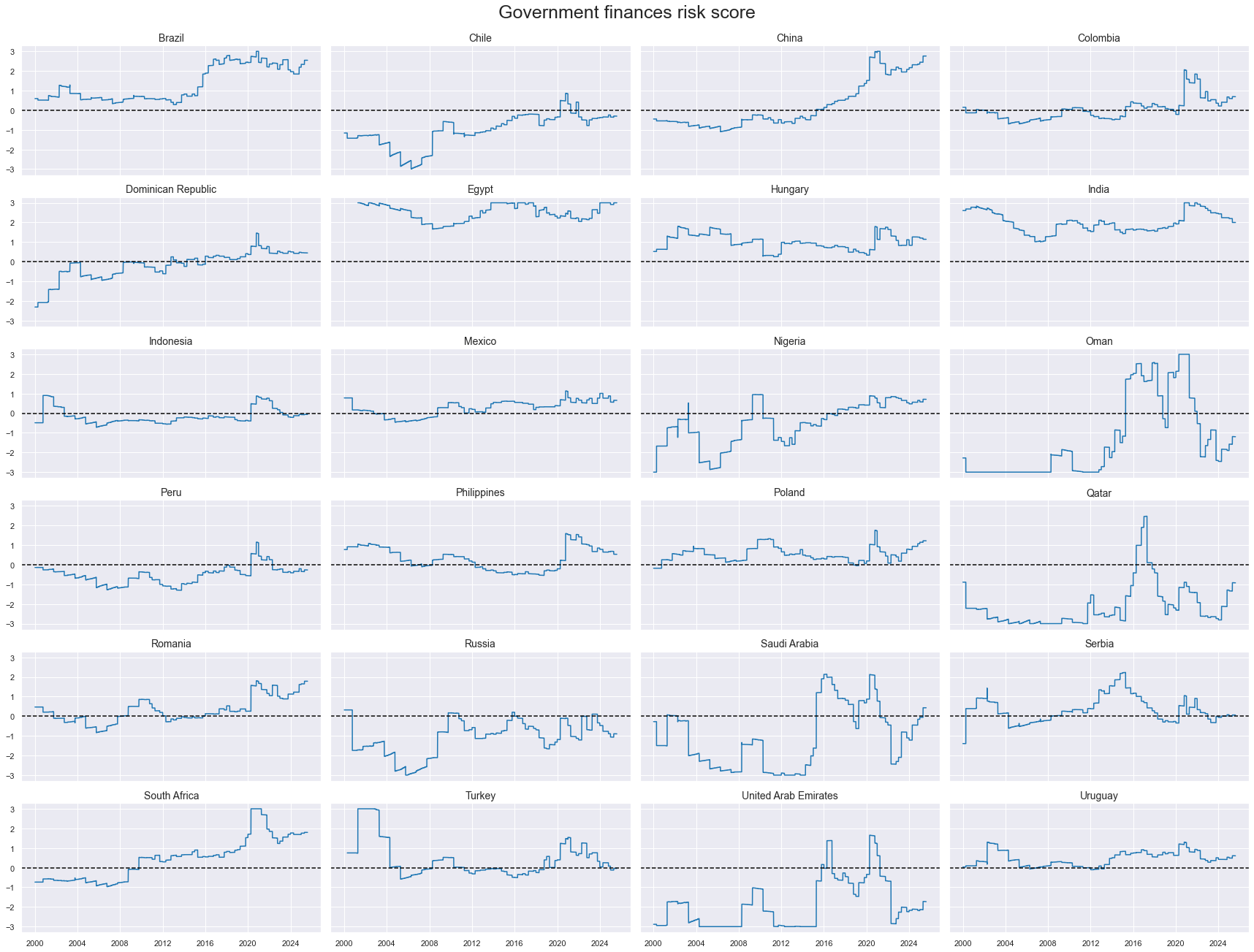
Label : Government finance risk score

Definition : General government finance risk score

Notes :

• The government finance risk score is a linear combination of z-scored government finance indicators.

• For general government finance risk, we use the general government balance as % of GDP for the current and next year, as well as the general government debt of the current year as % of GDP ( documentation here ).

• All else equal, lower balances, i.e., lower surpluses or higher deficits, and higher debt ratios imply a higher debt servicing burden and increase sovereign default risk.

• To compute macro risk scores, all indicators are first normalized sequentially using the median and standard deviation of the full panel— that is, all country time series values available up to a given point in time. To reduce the influence of outliers, values are capped at three standard deviations in both directions. Subsequently, indicator signs are adjusted so that a higher score consistently reflects higher macroeconomic risk.

Ticker : XBALRISK_NSA

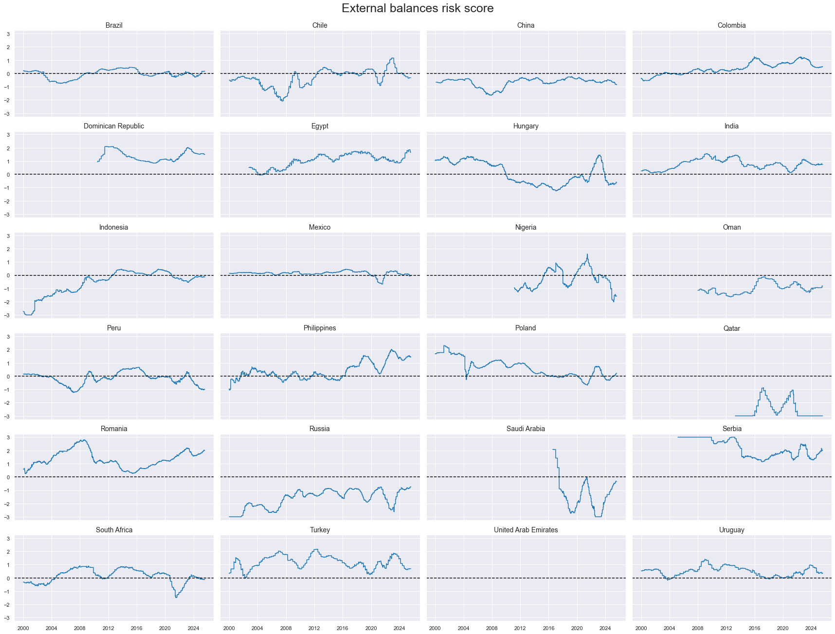
Label : External balance risk score

Definition : External balance risk score

Notes :

• The external balance risk score is a linear combination of z-scored external balance indicators.

• For external balance risk, we use the merchandise trade balance and the broader external current account, both as % of GDP and 12-month average ( documentation here ).

• All else equal, lower balances, i.e., smaller external surpluses or higher external deficits, increase the risk of currency depreciation and related surges of external debt servicing costs relative to local-currency tax revenues. Thereby, lower external balance ratios translate into higher sovereign default risk.

• To compute macro risk scores, all indicators are first normalized sequentially using the median and standard deviation of the full panel—that is, all country time series values available up to a given point in time. To reduce the influence of outliers, values are capped at three standard deviations in both directions. Subsequently, indicator signs are adjusted so that a higher score consistently reflects higher macroeconomic risk.

Ticker : XLIABRISK_NSA

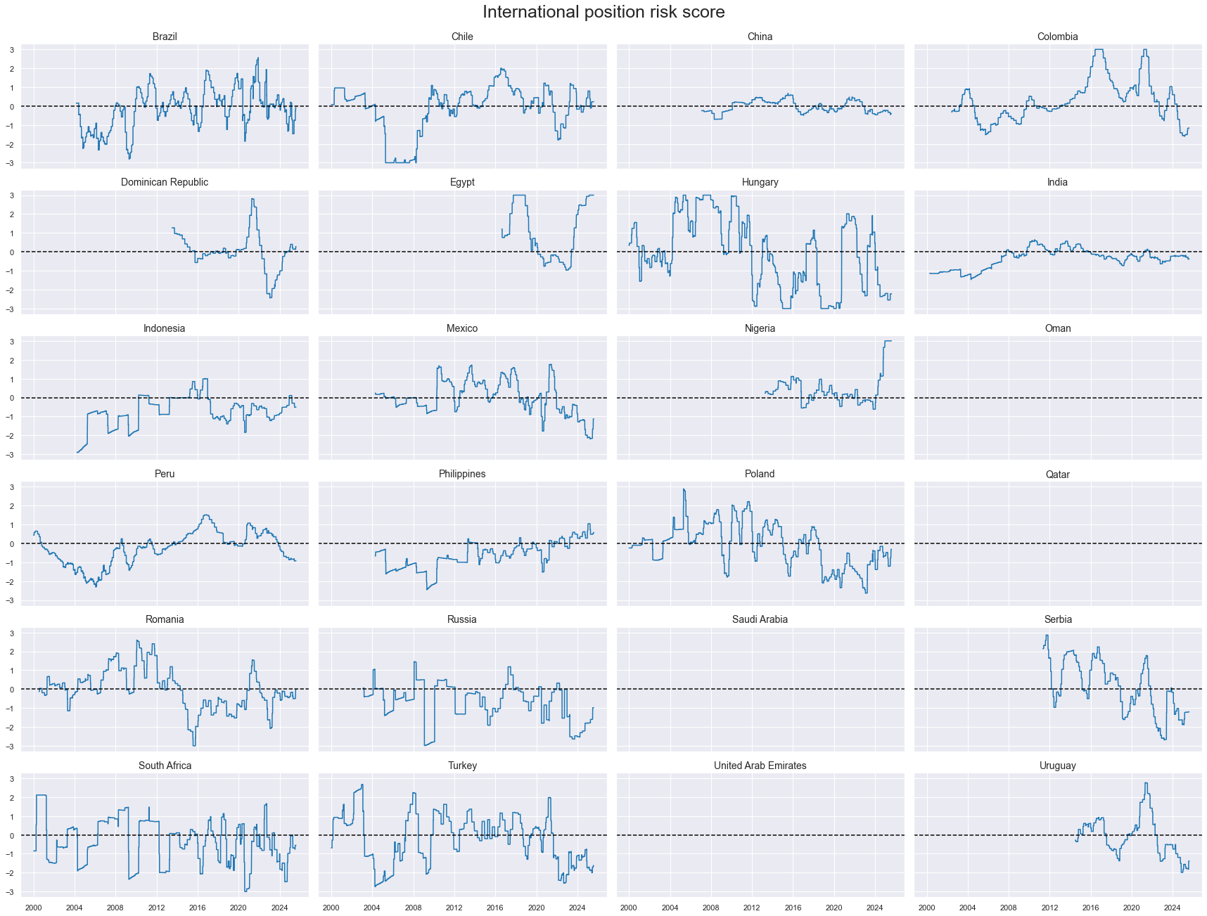
Label : International investment risk score

Definition : International investment risk score

Notes :

• The international investment score is a linear combination of z-scored international investment indicators.

• For international investment risk, we observe medium-term trends in cross-border investment positions. These include the difference between the latest net international investment position as % of GDP and its 2-year and 5-year moving averages, and the difference between the latest international liabilities ratios to GDP and their 2-year and 5-year moving averages - ( documentation here ). Declining net investment positions and rising liabilities point to growing dependence on foreign funding and rising vulnerability to sudden stops or reversals. Such vulnerability increases the risk of default across the economy.

• To compute macro risk scores, all indicators are first normalized sequentially using the median and standard deviation of the full panel—that is, all country time series values available up to a given point in time. To reduce the influence of outliers, values are capped at three standard deviations in both directions. Subsequently, indicator signs are adjusted so that a higher score consistently reflects higher macroeconomic risk.

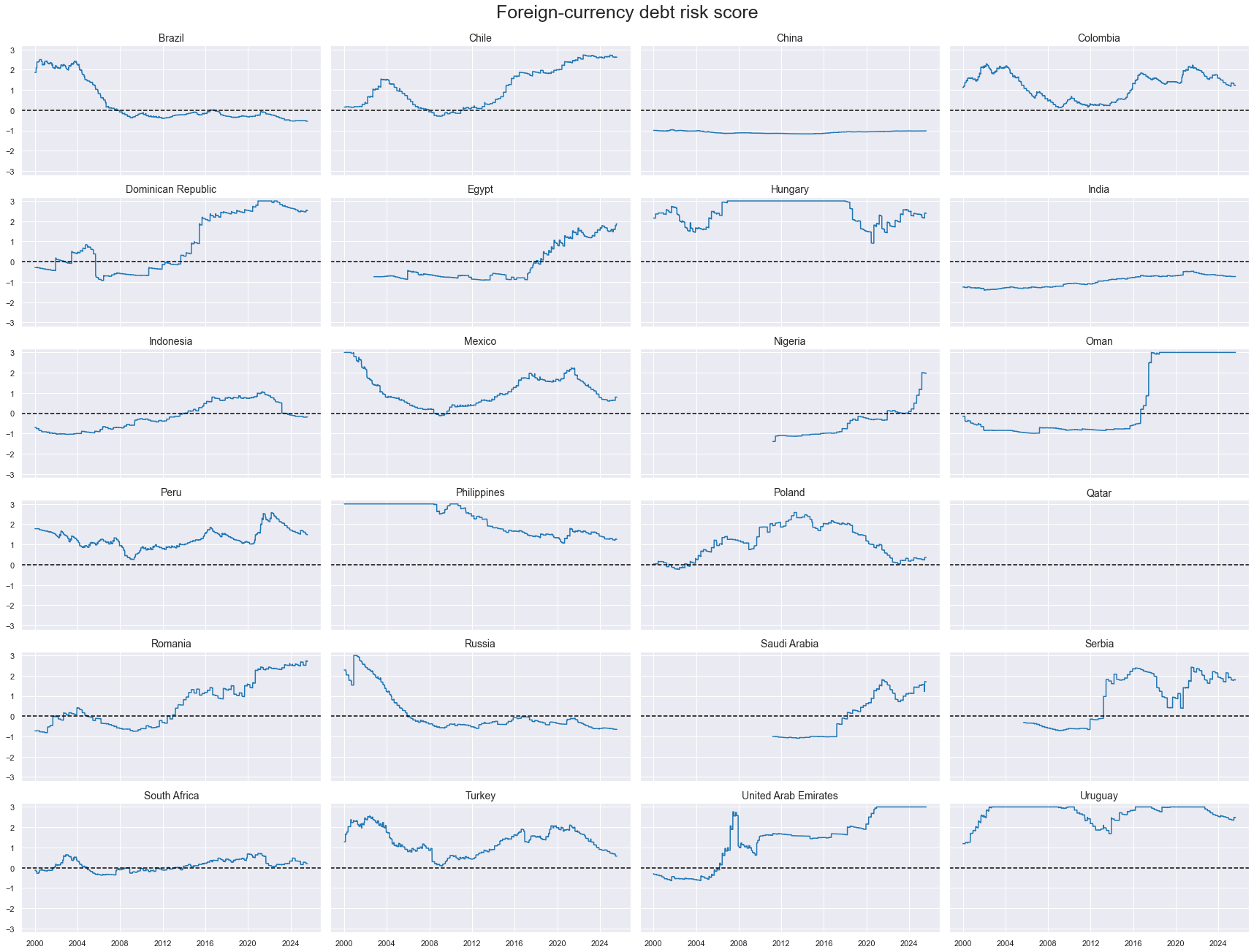
Ticker : XDEBTRISK_NSA

Label : Foreign debt sustainability risk score

Definition : Foreign debt sustainability score

Notes :

• The foreign debt sustainability score is a linear combination of z-scored foreign debt sustainability indicators.

• For foreign debt sustainability risk, we observe medium-term trends in cross-border investment positions. These include the difference between the latest net international investment position as % of GDP and its 2-year and 5-year moving averages, and the difference between the latest international liabilities ratios to GDP and their 2-year and 5-year moving averages ( documentation here ).

• Declining net investment positions and rising liabilities point to growing dependence on foreign funding and rising vulnerability to sudden stops or reversals. Such vulnerability increases the risk of default across the economy.

• To compute macro risk scores, all indicators are first normalized sequentially using the median and standard deviation of the full panel— that is, all country time series values available up to a given point in time. To reduce the influence of outliers, values are capped at three standard deviations in both directions. Subsequently, indicator signs are adjusted so that a higher score consistently reflects higher macroeconomic risk.

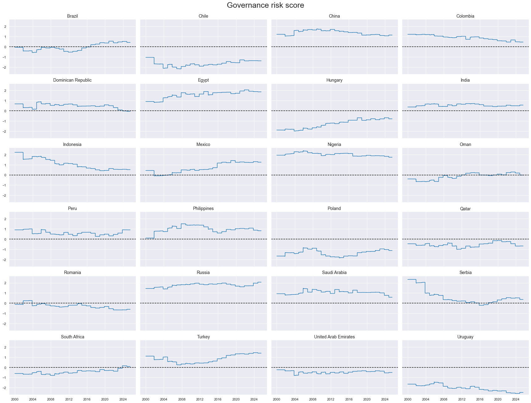
Ticker : GOVRISK_NSA

Label : Political stability and governance risk

Definition : Political stability and governance risk

Notes :

• The governance score is a linear combination of z-scored governance scores.

• For political stability and governance risk, we look at the governance scores of Transparency International and World Bank surveys. As a representative set we use indicators of government accountability, political stability and corruption control ( documentation here ). The poorer the governance of a country, the higher the risk of instability and default.

• To compute macro risk scores, all indicators are first normalized sequentially using the median and standard deviation of the full panel—that is, all country time series values available up to a given point in time. To reduce the influence of outliers, values are capped at three standard deviations in both directions. Subsequently, indicator signs are adjusted so that a higher score consistently reflects higher macroeconomic risk.

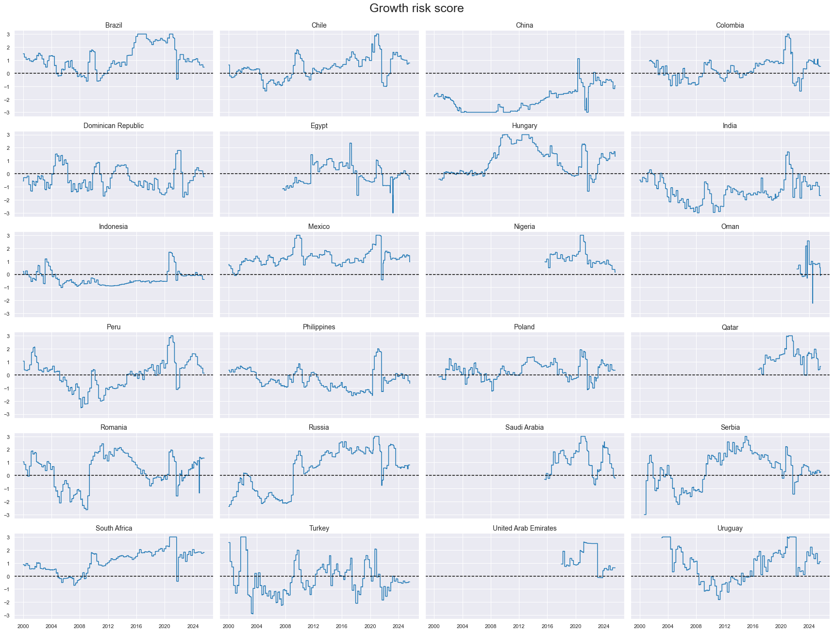
Ticker : GROWTHRISK_NSA

Label : Economic growth-related risk

Definition : Economic growth-related risk

Notes :

• The growth score is a linear combination of z-scored growth indicators.

• For economic growth-related risk, we use 5-year moving averages of real GDP growth. Persistently weaker growth typically translates into greater financial, economic, and political risk ( documentation here ).

• To compute macro risk scores, all indicators are first normalized sequentially using the median and standard deviation of the full panel—that is, all country time series values available up to a given point in time. To reduce the influence of outliers, values are capped at three standard deviations in both directions. Subsequently, indicator signs are adjusted so that a higher score consistently reflects higher macroeconomic risk.

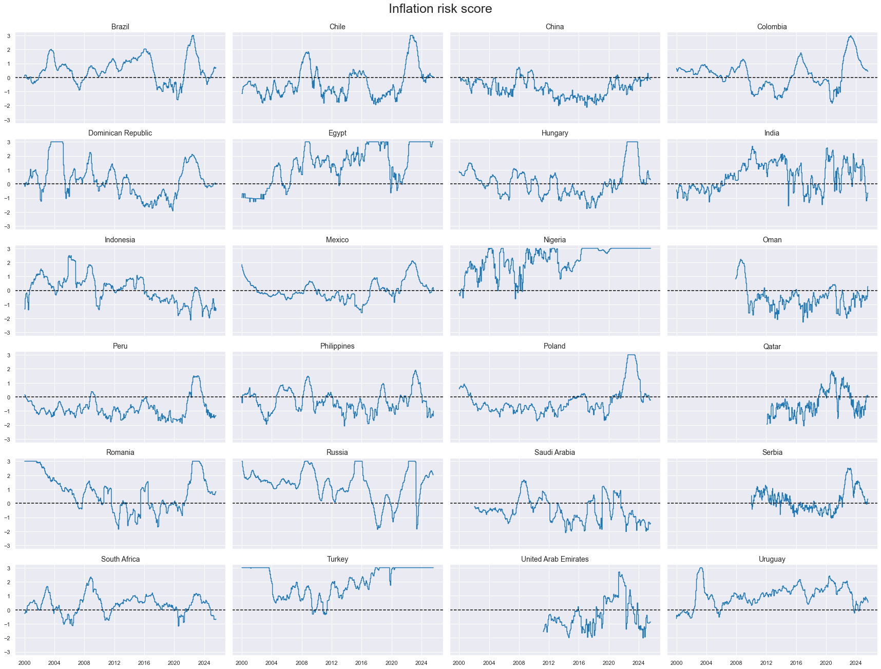
Ticker : INFLRISK_NSA

Label : Inflation risk score

Definition : Inflation risk score

Notes :

• The inflation score is a linear combination of z-scored inflation indicators.

• For inflation-related risk, we monitor core and headline CPI inflation ( documentation here ). To account for the two-sided and non-linear impact of inflation on financial stability — where incremental changes have diminishing marginal effects at higher inflation levels — we use the square root of the deviation of inflation rates from the conventional 2% target of developed markets.

• Both elevated inflation and deflation are considered sources of financial instability and, consequently, contribute to increased sovereign default risk.

• To compute macro risk scores, all indicators are first normalized sequentially using the median and standard deviation of the full panel—that is, all country time series values available up to a given point in time. To reduce the influence of outliers, values are capped at three standard deviations in both directions. Subsequently, indicator signs are adjusted so that a higher score consistently reflects higher macroeconomic risk.

Macro composite score

Ticker : MACROSCORE_NSA

Label : Composite macro risk score

Definition : Composite macro risk score

Notes :

• A composite macro risk score is a re-normalized average of the seven conceptual (macro) risk factor scores.

• Macro-quantamental risk scores represent normalized point-in-time information states of economic indicators related to the probability of fundamental losses, such as a creditor’s default. The term “quantamental” refers to meaningful quantitative-fundamental indicators whose relevance is supported by theory and experience. “Point-in-time” means that for each day in history, the indicator displays the latest publicly available updated value of the underlying concept.

• Thus, the composite macro risk score is the result of a linear combination of the re-normalised macro-quantamental risk scores shown above. In particular, it is a linear combination of the general government finance, external balance, international investment, foreign debt sustainability, political stability and governance, economic growth and inflation risk scores. The functions used to calculate the zn scores and linear combinations are those of the Macrosynergy package, ( outlined here and here ).

• A score of 1 in the macro composite indicates that, based solely on available macro indicators, a country’s sovereign risk is one standard deviation above normal, i.e., on the riskier side by historical and international standards.

• If some factors are missing, the composite is formed from the remaining ones, regardless of the number of factors present.

Imports

Only the standard Python data science packages and the specialized macrosynergy package are needed.

import numpy as np
import pandas as pd
from pandas import Timestamp
import matplotlib.pyplot as plt
import seaborn as sns
import os
import io

from datetime import datetime

import macrosynergy.management as msm
import macrosynergy.panel as msp
import macrosynergy.signal as mss
import macrosynergy.pnl as msn
import macrosynergy.visuals as msv

from macrosynergy.download import JPMaQSDownload
from macrosynergy.panel.adjust_weights import adjust_weights
import warnings

pd.set_option('display.width', 400)
pd.set_option('display.precision', 4)

warnings.simplefilter("ignore")

The JPMaQS indicators we consider are downloaded using the J.P. Morgan Dataquery API interface within the macrosynergy package. This is done by specifying ticker strings , formed by appending an indicator category code <category> to a currency area code <cross_section> . These constitute the main part of a full quantamental indicator ticker, taking the form DB(JPMAQS,<cross_section>_<category>,<info>) , where <info> denotes the time series of information for the given cross-section and category. The following types of information are available:

• value giving the latest available values for the indicator

• eop_lag referring to days elapsed since the end of the observation period

• mop_lag referring to the number of days elapsed since the mean observation period

• grade denoting a grade of the observation, giving a metric of real time information quality.

After instantiating the JPMaQSDownload class within the macrosynergy.download module, one can use the download(tickers,start_date,metrics) method to easily download the necessary data, where tickers is an array of ticker strings, start_date is the first collection date to be considered and metrics is an array comprising the times series information to be downloaded.

cids_fc_latam = [  # Latam foreign currency debt countries
    "BRL",
    "CLP",
    "COP",
    "DOP",
    "MXN",
    "PEN",
    "UYU",
]
cids_fc_emeu = [  # EM Europe foreign currency debt countries
    "HUF",
    "PLN",
    "RON",
    "RUB",
    "RSD",
    "TRY",
]
cids_fc_meaf = [  # Middle-East and Africa foreign currency debt countries
    "AED",
    "EGP",
    "NGN",
    "OMR",
    "QAR",
    "ZAR",
    "SAR",
]
cids_fc_asia = [  # Asia foreign currency debt countries
    "CNY",
    "IDR",
    "INR",
    "PHP",
]

cids_fc = sorted(
    list(
        set(cids_fc_latam + cids_fc_emeu + cids_fc_meaf + cids_fc_asia)
    )
)
cids_emxfc = ["CZK", "ILS", "KRW", "MYR", "SGD", "THB", "TWD"]

cids_em = sorted(cids_fc + cids_emxfc)

# Category tickers

risk_scores = ['GFINRISK_NSA','XBALRISK_NSA','XLIABRISK_NSA','XDEBTRISK_NSA','GOVRISK_NSA','GROWTHRISK_NSA','INFLRISK_NSA']

composite_risk_score = ['MACROSCORE_NSA'] 


risk_metrics = [
    "LTFCRATING_NSA",
    "FCBICRY_NSA",
    "FCBICRY_VT10",
    "CDS05YSPRD_NSA",
]

# Targets

rets = ["FCBIR_NSA", "FCBIXR_NSA", "FCBIXR_VT10"]


# Create ticker list

xcats = risk_metrics + rets + risk_scores + composite_risk_score
tickers = [cid + "_" + xcat for cid in cids_em for xcat in xcats]

print(f"Maximum number of tickers is {len(tickers)}")

Maximum number of tickers is 465

# Download series from J.P. Morgan DataQuery by tickers

start_date = "1998-01-01"
tickers = [cid + "_" + xcat for cid in cids_em for xcat in xcats]
print(f"Maximum number of tickers is {len(tickers)}")

# Retrieve credentials

client_id: str = os.getenv("DQ_CLIENT_ID")
client_secret: str = os.getenv("DQ_CLIENT_SECRET")

# Download from DataQuery

with JPMaQSDownload(client_id=client_id, client_secret=client_secret) as downloader:
    df = downloader.download(
        tickers=tickers,
        start_date=start_date,
        metrics=["value", "eop_lag", "mop_lag", "grading"],
        suppress_warning=True,
        show_progress=True,
    )

dfx = df

Maximum number of tickers is 465
Downloading data from JPMaQS.
Timestamp UTC:  2025-08-08 11:48:08
Connection successful!

Requesting data: 100%|██████████| 93/93 [00:18<00:00,  4.93it/s]
Downloading data: 100%|██████████| 93/93 [00:40<00:00,  2.31it/s]

Some expressions are missing from the downloaded data. Check logger output for complete list.
212 out of 1860 expressions are missing. To download the catalogue of all available expressions and filter the unavailable expressions, set `get_catalogue=True` in the call to `JPMaQSDownload.download()`.

black_fc = {'RUB': [Timestamp('2022-02-01 00:00:00'), Timestamp('2035-02-26 00:00:00')]}

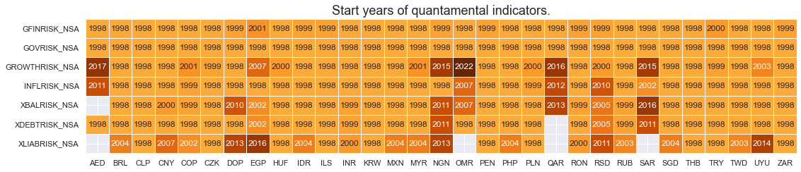
Availability

Most series are available from the late 1990s. USA and GBP data go back to the early 1990s. However, the U.S. has not published gross debt servicing data for the corporate and overall private sector. Korean data have only been available from 2011.

xcatx = risk_scores
msm.check_availability(df=dfx, xcats=xcatx, cids=cids_em, missing_recent=False)

xcatx = composite_risk_score
msm.check_availability(df=dfx, xcats=xcatx, cids=cids_em, missing_recent=False)

Vintage quality has been very different across countries. For most countries JPMaQS has only a few recent years of original vintages. This includes Switzerland, the UK, and the U.S. (for household debt services).

History

Macro scores

dict_labels = {}
dict_labels["GFINRISK_NSA"] = "Government finances risk score"
dict_labels["XBALRISK_NSA"] = "External balances risk score"
dict_labels["XLIABRISK_NSA"] = "International position risk score"
dict_labels["XDEBTRISK_NSA"] = "Foreign-currency debt risk score"
dict_labels['GOVRISK_NSA'] = 'Governance risk score'
dict_labels['GROWTHRISK_NSA'] = "Growth risk score"
dict_labels["INFLRISK_NSA"] = "Inflation risk score"
dict_labels['MACROSCORE_NSA'] = "Composite macro score"

dict_countries = {
    'AED': 'United Arab Emirates',
    'BRL': 'Brazil',
    'CLP': 'Chile',
    'CNY': 'China',
    'COP': 'Colombia',
    'DOP': 'Dominican Republic',
    'EGP': 'Egypt',
    'HUF': 'Hungary',
    'IDR': 'Indonesia',
    'INR': 'India',
    'MXN': 'Mexico',
    'NGN': 'Nigeria',
    'OMR': 'Oman',
    'PEN': 'Peru',
    'PHP': 'Philippines',
    'PLN': 'Poland',
    'QAR': 'Qatar',
    'RON': 'Romania',
    'RSD': 'Serbia',
    'RUB': 'Russia',
    'SAR': 'Saudi Arabia',
    'TRY': 'Turkey',
    'UYU': 'Uruguay',
    'ZAR': 'South Africa'
}

All factor scores are highly autocorrelated, and some more structural factors maintain positive or negative values for a decade or longer.

for score in risk_scores:
    xcatx = [score]
    title = dict_labels[xcatx[0]]
    cidx = cids_fc
    sdate = "2000-01-01"
    
    msp.view_timelines(
        dfx,
        xcats=xcatx,
        cids=cidx,
        ncol=4,
        start=sdate,
        same_y=True,
        aspect=2,
        xcat_labels=dict_labels,
        cid_labels=dict_countries,
        title=f"{title}",
        title_fontsize=25,
        legend_fontsize=16,
        height=2,
    )

sub_risk_scores = ['GFINRISK_NSA', 'XLIABRISK_NSA'] 
sub_cids = ['AED', 'BRL', 'CLP', 'CNY', 'COP', 'DOP', 'EGP']


msp.correl_matrix(
    df=dfx,
    xcats=[sub_risk_scores[0]],
    xcats_secondary=[sub_risk_scores[1]],
    cids=sub_cids,
    title=f"Correlation matrix of {dict_labels[sub_risk_scores[0]]} and {dict_labels[sub_risk_scores[1]]}, select cross-sections, since 2000",
)

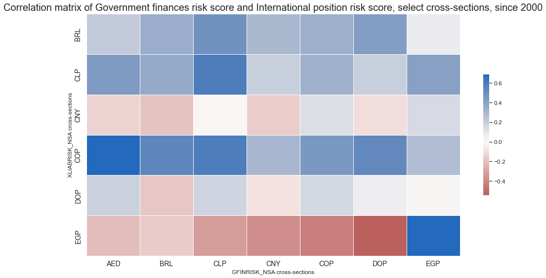
Correlations between macro scores have been generally positive across the analised horizon.

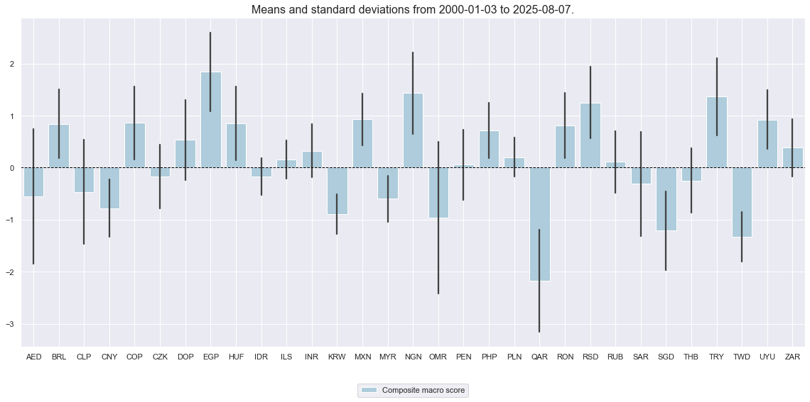
xcatx = ['MACROSCORE_NSA']
cidx = cids_fc
sdate = "2000-01-01"

msp.view_ranges(
    dfx,
    xcats=xcatx,
    kind="bar",
    sort_cids_by=None,
    start=sdate,
    xcat_labels=dict_labels,
)

msp.view_timelines(
    dfx,
    xcats=xcatx,
    cids=cidx,
    ncol=4,
    start=sdate,
    same_y=True,
    aspect=2,
    xcat_labels=dict_labels,
    cid_labels=dict_countries,
    title="Composite macro risk related to sovereign risk, equally-weighted score of 7 constituents",
    title_fontsize=25,
    legend_fontsize=16,
    height=2,
)

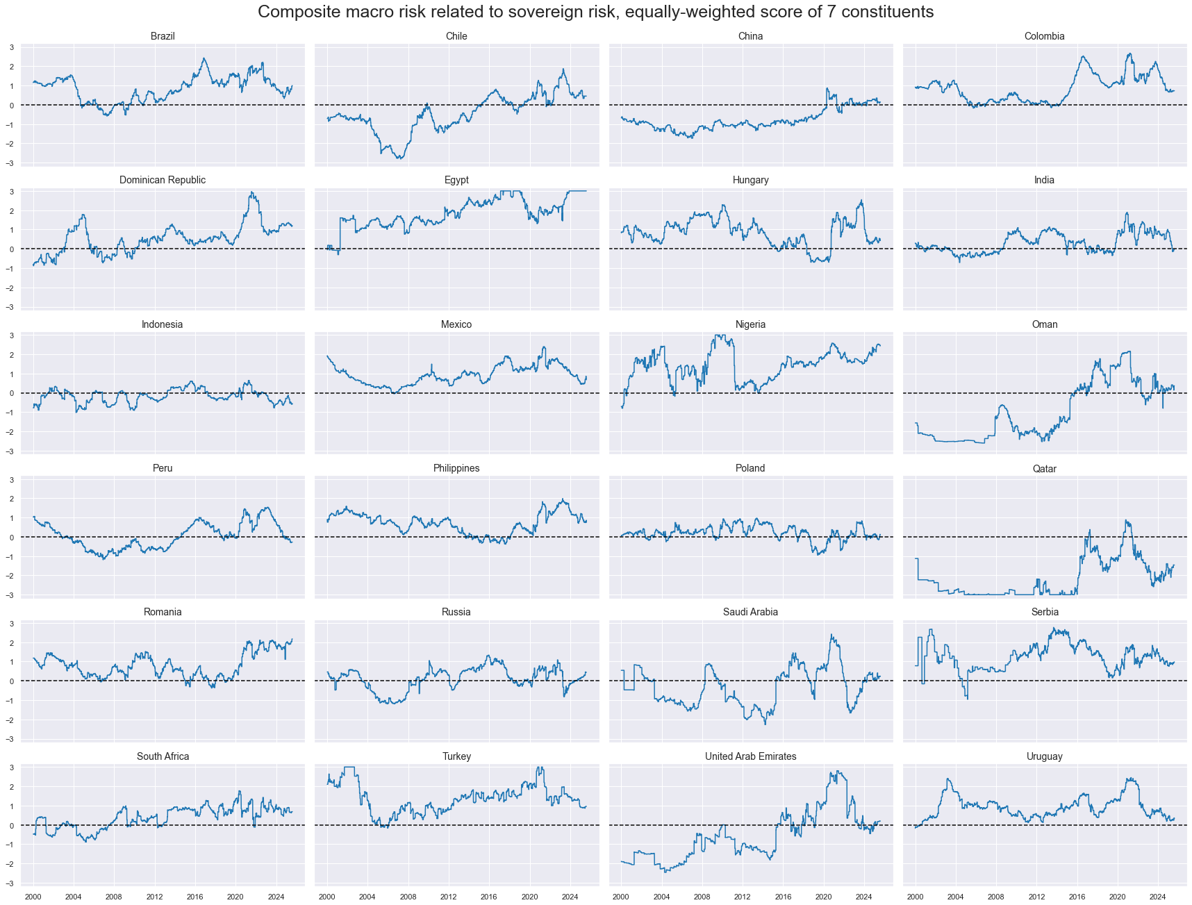
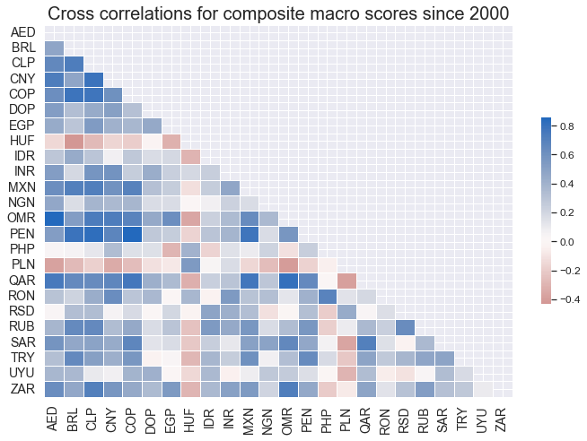
A composite macro risk score is a re-normalized average of the seven conceptual risk factor scores. If some factors are missing, the composite is formed from the remaining ones, regardless of the number of factors present. Generally, composite macro scores are highly correlated among countries.

cidx = cids_fc

msp.correl_matrix(
    dfx,
    xcats="MACROSCORE_NSA",
    cids=cidx,
    size=(10, 7),
    start="2000-01-01",
    title="Cross correlations for composite macro scores since 2000",
)

Importance

Research links

Macro risk premium scores estimate the price-value gaps of financial contracts, both relative to historical benchmarks and in comparison with one another. Combining market and macroeconomic information offers a structured, intelligent approach to leveraging quantitative date, often yielding more substantial and reliable value than unstructured uses of the individual data sets. The importance of clear theoretical priors is illustrated by the simple credit risk model presented below. Macrosynergy .

Empirical clues

We aim to show the relationships between our composite macro scores and two proxies of market risk scores. We approximate the market’s required compensation for sovereign credit risk by two metrics, with complementary strengths.

We then aim to build risk-premium scores, as per the Macrosynergy research post here . Macro risk premium scores, derived from this comparison, capture variations in premia paid across time and countries. Applied to 24 sovereigns over the past 25 years, these scores show significant positive predictive power for volatility-targeted returns on U.S. dollar-denominated bond indices.

With regards to the market risk scores, we use two indications of such risk:

Log sovereign spread scores are normalized natural logarithms of 5-year credit default swap (CDS) spreads ( documentation here ) using medians and standard deviations of the 24-country panel up to each point in time. As for macro factors, the scores are winsorized at three standard deviations. For the ten sovereigns without a liquid CDS market, spreads are approximated by the foreign-currency bond index carry ( documentation here ). Logarithms are used because credit spreads tend to increase more than proportionally with rising default probability. This is due to the convex relationship between spreads and default risk, and is akin to option pricing. The non-linearity is also evident in the empirical relationships between sovereign credit spreads and both ratings and macro risk indices in our 24-country data panel.

Ratings scores are based on long-term foreign-currency sovereign credit rating indices. These indices are calculated as weighted averages of ratings and outlook data of Fitch, S&P, and Moody’s ( documentation here ). The values go from 1 to 23, with a higher value indicating a better rating. However, for the purpose of risk scores, we have inverted numeric values so that higher values indicate higher risk, analogously to spreads.

# Use index carry where CDS spreads not available ("priced risk" score)

msm.missing_in_df(df, xcats=["CDS05YSPRD_NSA"], cids=cids_fc)  # countries without CDS
cidx = ['AED', 'DOP', 'EGP', 'INR', 'NGN', 'OMR', 'QAR', 'RSD', 'SAR', 'UYU']

calcs = ["CDS05YSPRD_NSA = FCBICRY_NSA"]
dfa = msp.panel_calculator(dfx, calcs=calcs, cids=cidx)
dfx = msm.update_df(dfx, dfa)

# Use inverse rating score ("rated risk" score)

calcs = [
    "LTFCRATING_ADJ = LTFCRATING_NSA + 1",  # temporary fix for VEF/RUB problem
    "LTFCRATING_INV = 1 / LTFCRATING_ADJ",
    "CDS05YSPRD_LOG = np.log( CDS05YSPRD_NSA )"  # accoount for non-linearity of spread changes
]
cidx = cids_fc
dfa = msp.panel_calculator(dfx, calcs=calcs, cids=cidx)
dfx = msm.update_df(dfx, dfa)

No missing XCATs across DataFrame.
Missing cids for CDS05YSPRD_NSA:  ['AED', 'DOP', 'EGP', 'INR', 'NGN', 'OMR', 'QAR', 'RSD', 'SAR', 'UYU']

# Re-score the composite

for xc in ["CDS05YSPRD_LOG", "LTFCRATING_INV"]:
    dfa = msp.make_zn_scores(
        dfx,
        xcat=xc,
        cids=cidx,
        sequential=True,
        min_obs=261 * 3,
        neutral="median",
        pan_weight=1,
        thresh=3,
        postfix="_ZN",
        est_freq="m",
    )
    
    dfx = msm.update_df(dfx, dfa)

dict_labels["CDS05YSPRD_LOG_ZN"] = "Log spread-based market risk score"
dict_labels["LTFCRATING_INV_ZN"] = "Ratings-based market risk score"

# Composite market risk scores

cidx = cids_fc
xcatx = ["CDS05YSPRD_LOG_ZN", "LTFCRATING_INV_ZN"]

dfa = msp.linear_composite(
    dfx,
    xcats=xcatx,
    cids=cidx,
    complete_xcats=False,
    new_xcat="MARKETRISK",
)

dfx = msm.update_df(dfx, dfa)

# Re-score the composite

dfa = msp.make_zn_scores(
    dfx,
    xcat="MARKETRISK",
    cids=cidx,
    sequential=True,
    min_obs=261 * 3,
    neutral="zero",
    pan_weight=1,
    thresh=3,
    postfix="_ZN",
    est_freq="m",
)

dfx = msm.update_df(dfx, dfa)

dict_labels["MARKETRISK_ZN"] = "Composite market risk score"

xcatx = ["LTFCRATING_INV_ZN", "CDS05YSPRD_LOG_ZN"]
cidx = cids_fc

cr = msp.CategoryRelations(
    dfx,
    xcats=xcatx,
    cids=cidx,
    years=5,
    lag=0,
    xcat_aggs=["mean", "mean"],
    blacklist=black_fc,
    start="2000-01-01",
)

cr.reg_scatter(
    labels=True,
    label_fontsize=12,
    title="Long-term relations between credit spread and rated risk scores, by half-decades, since 2000",
    title_fontsize=16,
    xlab="Rated risk score, half-decade average",
    ylab="Credit spread score, half-decade average",
)

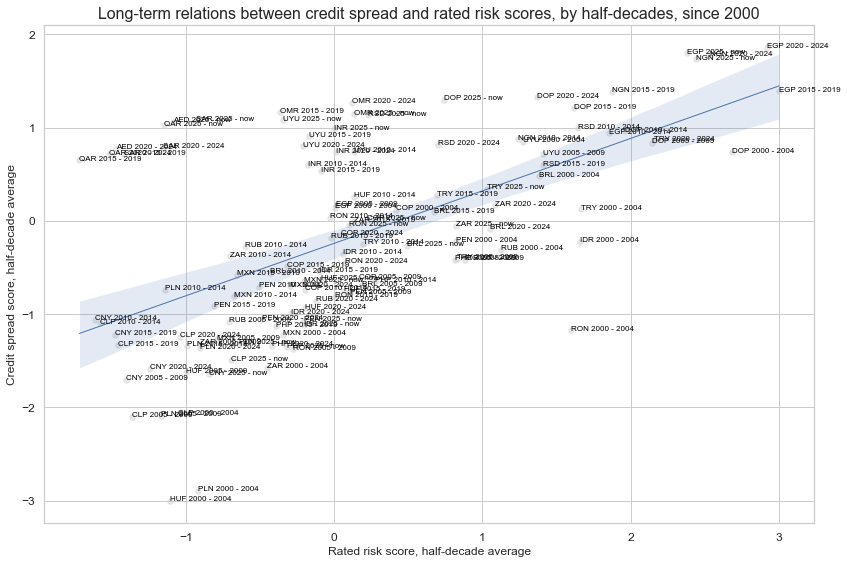
Sovereign credit-related macro risk scores have been strongly positively correlated with ratings-based market risk scores.

# Long-term macro risk - ratings relations

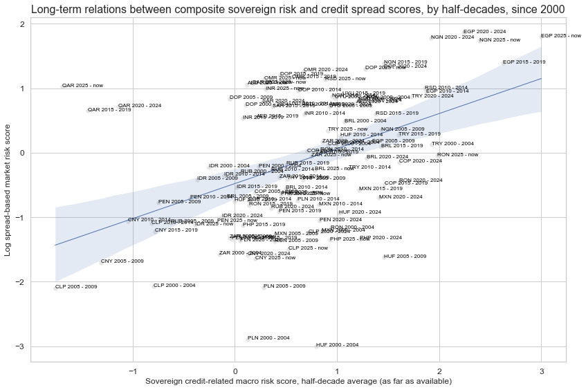
xcatx = ["MACROSCORE_NSA", "CDS05YSPRD_LOG_ZN"]
cidx = cids_fc

cr = msp.CategoryRelations(
    dfx,
    xcats=xcatx,
    cids=cidx,
    years=5,
    lag=0,
    xcat_aggs=["mean", "mean"],
    blacklist=black_fc,
    start="2000-01-01",
)

cr.reg_scatter(
    labels=True,
    label_fontsize=12,
    title="Long-term relations between composite sovereign risk and credit spread scores, by half-decades, since 2000",
    title_fontsize=16,
    xlab="Sovereign credit-related macro risk score, half-decade average (as far as available)",
    ylab=dict_labels['CDS05YSPRD_LOG_ZN'],
)

# Long-term macro risk - ratings relations

xcatx = ["MACROSCORE_NSA", "LTFCRATING_INV_ZN"]
cidx = cids_fc

cr = msp.CategoryRelations(
    dfx,
    xcats=xcatx,
    cids=cidx,
    years=5,
    lag=0,
    xcat_aggs=["mean", "mean"],
    blacklist=black_fc,
    start="2000-01-01",
)

cr.reg_scatter(
    labels=True,
    label_fontsize=12,
    title="Long-term relations between composite sovereign risk and rated risk scores, by half-decades, since 2000",
    title_fontsize=16,
    xlab="Sovereign credit-related macro risk score, half-decade average (as far as available)",
    ylab=dict_labels['LTFCRATING_INV_ZN'],
)

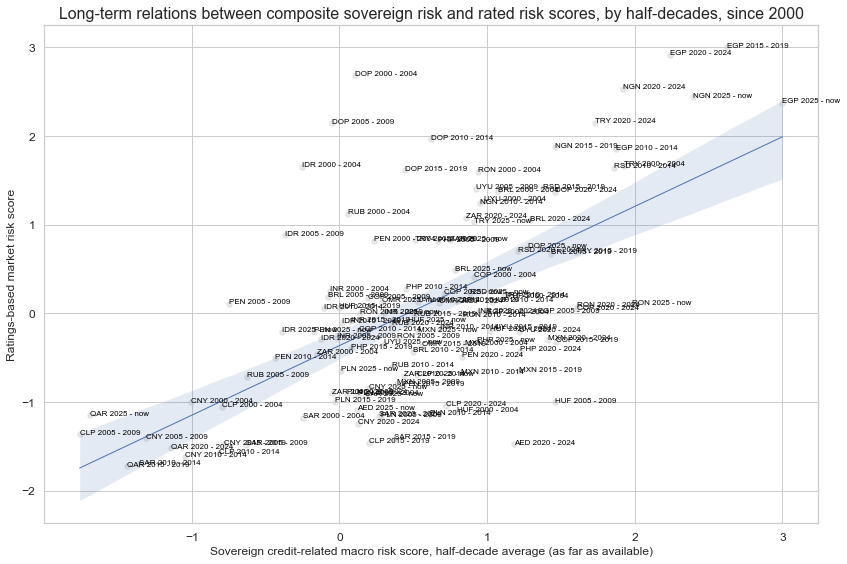
Long term relations between composite macro risk scores and credit spread scores, and composite macro risk scores and rated risk scores have been largely positive and statistically significant.

We now proceed to build our macro risk premium.

# Score differences

cidx = cids_fc

calcs = [
    "MACROSPREAD_RPS = CDS05YSPRD_LOG_ZN - MACROSCORE_NSA",
    "MACRORATING_RPS = LTFCRATING_INV_ZN - MACROSCORE_NSA",
    "MACROALL_RPS = MARKETRISK_ZN - MACROSCORE_NSA",
]
dfa = msp.panel_calculator(dfx, calcs=calcs, cids=cidx)
dfx = msm.update_df(dfx, dfa)

rps = list(dfa['xcat'].unique())

# Re-z-scoring the risk premium scores

for rp in rps:
    dfa = msp.make_zn_scores(
        dfx,
        xcat=rp,
        cids=cidx,
        sequential=True,
        min_obs=261 * 3,
        neutral="zero",
        pan_weight=1,
        thresh=3,
        postfix="_ZN",
        est_freq="m",
    )
    dfx = msm.update_df(dfx, dfa)

dict_labels["MACROSPREAD_RPS_ZN"] = "Spread-based macro risk premium score"
dict_labels["MACRORATING_RPS_ZN"] = "Ratings-based macro risk premium score"
dict_labels["MACROALL_RPS_ZN"] = "Macro risk premium score"

rpz = ["MACROSPREAD_RPS_ZN", "MACRORATING_RPS_ZN", "MACROALL_RPS_ZN",]
xrpz = rpz + [rp[:-3] + "_CWS_ZN" for rp in rpz]

dict_dir = {
    "sigs": ['MACROSPREAD_RPS_ZN','MACRORATING_RPS_ZN', 'MACROALL_RPS_ZN', 'MARKETRISK_ZN'],
    "targs": ["FCBIXR_VT10", "FCBIXR_NSA"],
    "cidx": cids_fc,
    "start": "2000-01-01",
    "black": black_fc,
}

dix = dict_dir

sigs = dix['sigs']
ret = dix["targs"][0]
cidx = dix["cidx"]
start = dix["start"]
black = dix["black"]

catregs = {}
for sig in sigs:
    catregs[sig] = msp.CategoryRelations(
        dfx,
        xcats=[sig, ret],
        cids=cidx,
        freq="M",
        lag=1,
        xcat_aggs=["last", "sum"],
        start=start,
        blacklist=black,
    )

msv.multiple_reg_scatter(
    cat_rels=[v for k, v in catregs.items()],
    ncol=2,
    nrow=2,
    figsize=(14, 12),
    title="Risk scores and subsequent foreign currency bond index excess returns, 24 countries since 2000",
    title_fontsize=20,
    xlab="End-of-quarter score",
    ylab="Foreign currency bond index excess returns, vol targeted, %, next quarter",
    coef_box="lower right",
    prob_est="map",
    single_chart=True,
    subplot_titles=[dict_labels[key] for key in sigs]
)

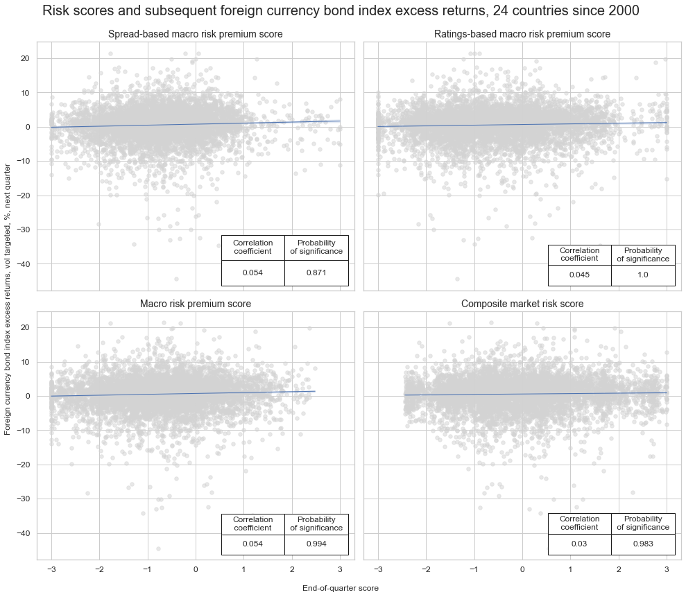
Both the spread-based macro risk premium and the ratings-based macro risk premiums are positively and significatly correlated with lagged foreign currency bond index returns. So is the market risk score, and, more importantly, we observe a strong positive correlation between our macro risk premium score and our returns, as a result of the previous relations.

Appendices

Appendix 1: Currency symbols

The word ‘cross-section’ refers to currencies, currency areas or economic areas. In alphabetical order, these are AUD (Australian dollar), BRL (Brazilian real), CAD (Canadian dollar), CHF (Swiss franc), CLP (Chilean peso), CNY (Chinese yuan renminbi), COP (Colombian peso), CZK (Czech Republic koruna), DEM (German mark), ESP (Spanish peseta), EUR (Euro), FRF (French franc), GBP (British pound), HKD (Hong Kong dollar), HUF (Hungarian forint), IDR (Indonesian rupiah), ITL (Italian lira), JPY (Japanese yen), KRW (Korean won), MXN (Mexican peso), MYR (Malaysian ringgit), NLG (Dutch guilder), NOK (Norwegian krone), NZD (New Zealand dollar), PEN (Peruvian sol), PHP (Phillipine peso), PLN (Polish zloty), RON (Romanian leu), RUB (Russian ruble), SEK (Swedish krona), SGD (Singaporean dollar), THB (Thai baht), TRY (Turkish lira), TWD (Taiwanese dollar), USD (U.S. dollar), ZAR (South African rand).