Labor market surprises

This category group contains economic surprise indicators related to levels and dynamics in employment and unemployment. Economic surprises are deviations of point-in-time quantamental indicators from predicted values. For an in-depth explanation, please read Appendix 2 .

Employment growth surprises

Ticker : EMPL_SA_P1M1ML12_ARMAS / _P1M1ML12_3MMA_ARMAS / _P1Q1QL4_ARMAS

Label : Employment, sa, %oya: ARMA(1,1)-based surprises / 3mma, ARMA(1,1)-based surprises / quarterly, ARMA(1,1)-based surprises

Definition : Employment, seasonally adjusted, % over a year ago: ARMA(1,1)-based surprises / 3mma, ARMA(1,1)-based surprises / quarterly, ARMA(1,1)-based surprises

Notes :

• Refer to the section on employment growth for notes on the underlying data series.

• Expected values for release dates are based on an “ARMA(1,1)” model. This is a simple univariate time series model that predicts increments based on an autoregressive component, i.e., last period’s value, and a moving average component, represented by last period’s error. The coefficients of the model are estimated sequentially based on the vintages of the underlying data. And each vintage-specific model produces a one-step-ahead forecast for the subsequent observation period.

• In contrast to the employment growth indicators themselves, the employment growth surprise indicators use seasonally adjusted series, simplifying one-period-ahead forecasts. However, since the transformation is a year-over-year percentage change, this seasonal adjustment has little practical impact on the results.

Unemployment rate surprises

Ticker : UNEMPLRATE_SA_ARMAS / UNEMPLRATE_SA_3MMA_ARMAS

Label : Unemployment rate, sa, ARMA(1,1)-based surprises: level / 3mma

Definition : Unemployment rate, seasonally adjusted, ARMA(1,1)-based surprises: level / 3-month moving average

Notes :

• Refer to the section on unemployment rates for notes on the underlying data series.

• Expected values for release dates are based on an “ARMA(1,1)” model. This is a simple univariate time series model that predicts increments based on an autoregressive component, i.e., last period’s value, and a moving average component, represented by last period’s error. The coefficients of the model are estimated sequentially based on the vintages of the underlying data. And each vintage-specific model produces a one-step-ahead forecast for the subsequent observation period.

• For CLP, COP, MYR, and TRY, longer historical data exist at mixed frequencies (quarterly and annual). To ensure consistency in surprise calculation, the series have been truncated to retain only a single frequency.

Unemployment growth surprises

Ticker : UNEMPLRATE_SA_3MMA_D1M1ML12_ARMAS / _D1Q1QL4_ARMAS

Label : Unemployment rate, sa, diff oya: 3mma, ARMA(1,1)-based surprises / quarterly, ARMA(1,1)-based surprises

Definition : Unemployment rate, seasonally adjusted, difference over a year ago: 3mma, ARMA(1,1)-based surprises / quarterly, ARMA(1,1)-based surprises

Notes :

• Refer to the section on unemployment growth for notes on the underlying data series.

• Expected values for release dates are based on an “ARMA(1,1)” model. This is a simple univariate time series model that predicts increments based on an autoregressive component, i.e., last period’s value, and a moving average component, represented by last period’s error. The coefficients of the model are estimated sequentially based on the vintages of the underlying data. And each vintage-specific model produces a one-step-ahead forecast for the subsequent observation period.

• For CLP, COP, MYR, and TRY, longer historical data exist at mixed frequencies (quarterly and annual). To ensure consistency in surprise calculation, the series have been truncated to retain only a single frequency.

Ticker : UNEMPLRATE_SA_D3M3ML3_ARMAS / _D6M6ML6_ARMAS / _D1Q1QL1_ARMAS / _D2Q2QL2_ARMAS

Label : Unemployment rate, sa: diff 3m/3m, ARMA(1,1)-based surprises / diff 6m/6m, ARMA(1,1)-based surprises / diff 1q/1q, ARMA(1,1)-based surprises / diff 2q/2q, ARMA(1,1)-based surprises

Definition : Unemployment rate, seasonally adjusted: difference 3 months over 3 months, ARMA(1,1)-based surprises / difference 6 months over 6 months, ARMA(1,1)-based surprises / difference quarter over quarter, ARMA(1,1)-based surprises / difference 2 quarters over 2 quarters, ARMA(1,1)-based surprises

Notes :

• Refer to the section on unemployment growth for notes on the underlying data series.

• Expected values for release dates are based on an “ARMA(1,1)” model. This is a simple univariate time series model that predicts increments based on an autoregressive component, i.e., last period’s value, and a moving average component, represented by last period’s error. The coefficients of the model are estimated sequentially based on the vintages of the underlying data. And each vintage-specific model produces a one-step-ahead forecast for the subsequent observation period.

• For CLP, COP, MYR, and TRY, longer historical data exist at mixed frequencies (quarterly and annual). To ensure consistency in surprise calculation, the series have been truncated to retain only a single frequency.

Unemployment gap surprises

Ticker : UNEMPLRATE_SA_3MMAv5YMA_ARMAS / _3MMAv10YMA_ARMAS / _3MMAv5YMM_ARMAS / _3MMAv10YMM_ARMAS

Label : Unemployment rate, sa: 3mma vs 5yma, ARMA(1,1)-based surprises / 3mma vs 10yma, ARMA(1,1)-based surprises / 3mma vs 5ymm, ARMA(1,1)-based surprises / 3mma vs 10ymm, ARMA(1,1)-based surprises

Definition : Unemployment rate, seasonally adjusted: 3-month moving average minus the 5-year moving average, ARMA(1,1)-based surprises / 3-month moving average minus the 10-year moving average, ARMA(1,1)-based surprises / 3-month moving average minus the 5-year moving median, ARMA(1,1)-based surprises / 3-month moving average minus the 10-year moving median, ARMA(1,1)-based surprises

Notes :

• Refer to the section on unemployment gaps for notes on the underlying data series.

• Expected values for release dates are based on an “ARMA(1,1)” model. This is a simple univariate time series model that predicts increments based on an autoregressive component, i.e., last period’s value, and a moving average component, represented by last period’s error. The coefficients of the model are estimated sequentially based on the vintages of the underlying data. And each vintage-specific model produces a one-step-ahead forecast for the subsequent observation period.

• For CLP, COP, MYR, and TRY, longer historical data exist at mixed frequencies (quarterly and annual). To ensure consistency in surprise calculation, the series have been truncated to retain only a single frequency.

Imports

Only the standard Python data science packages and the specialized macrosynergy package are needed.

import os
import numpy as np
import pandas as pd
import matplotlib.pyplot as plt
import seaborn as sns
from typing import List, Dict

import macrosynergy.management as msm
import macrosynergy.panel as msp
import macrosynergy.signal as mss
import macrosynergy.pnl as msn
import macrosynergy.visuals as msv

from macrosynergy.download import JPMaQSDownload

import warnings
warnings.simplefilter("ignore")

The JPMaQS indicators are retrieved using the J.P. Morgan DataQuery API via the macrosynergy package. Tickers are constructed by combining a currency area code ( <cross_section> ) with an indicator category code ( <category> ), forming a string of the form <cross_section>_<category> .

This composite string is embedded within a full DataQuery ticker:

DB(JPMAQS,<cross_section>_<category>,<info>)

where <info> refers to the type of time series data requested. The available options are:

• value : the latest available value of the indicator

• eop_lag : days since the end of the observation period

• mop_lag : days since the mean observation period

• grade : a real-time data quality metric

To download data, instantiate the JPMaQSDownload class from macrosynergy.download , and use the .download(tickers, start_date, metrics) method, where:

• tickers is a list of constructed ticker strings

• start_date is the first collection date to retrieve

• metrics specifies the types of information (e.g. value , grade ) to download

The macrosynergy package makes it easy to retrieve and work with this data in a fully programmatic and repeatable way.

# Cross-sections of interest

cids_dmca = ["AUD","CAD","CHF","EUR","GBP","JPY","NOK","NZD","SEK","USD"]  # DM currency areas
cids_dmec = ["DEM", "ESP", "FRF", "ITL", "NLG"]  # DM euro area countries
cids_latm = ["BRL", "COP", "CLP", "MXN", "PEN"]  # Latam countries
cids_emea = ["CZK", "HUF", "PLN", "RON", "RUB", "TRY", "ZAR"]  # EMEA countries
cids_emas = ["CNY","HKD","IDR","INR","KRW","MYR","PHP","SGD","THB","TWD"]  # EM Asia countries

cids_dm = cids_dmca + cids_dmec
cids_em = cids_latm + cids_emea + cids_emas

# For Equity analysis:

cids_g3 = ["EUR", "JPY", "USD"]  # DM large currency areas
cids_dmes = ["AUD", "CAD", "CHF", "GBP", "SEK"]  # Smaller DM equity countries
cids_dmeq = cids_g3 + cids_dmes  # DM equity countries

# For FX analysis:
cids_nofx = ["USD", "EUR", "CNY", "SGD", "HKD"]
cids_dmfx = list(set(cids_dmca) - set(cids_nofx)) # DM currencies excluding USD, EUR
cids_emfx = list(set(cids_em) - set(cids_nofx))


cids = sorted(cids_dm + cids_em)
cids_lab = sorted(list(set(cids) - set(["CNY", "IDR", "INR"])))
cids_rgdppe = sorted(list(set(cids) - set(cids_dmec + ["HKD"])))

# Quantamental categories of interest

xcats_empl = [
    f"EMPL_SA_{transformation}_ARMAS" for transformation in 
    [
        "P1M1ML12",
        "P1M1ML12_3MMA",
        "P1Q1QL4",
    ]]

xcats_unempl = sorted([
    f"UNEMPLRATE_SA{transformation}_ARMAS" for transformation in 
    [
        "",
        "_3MMA_D1M1ML12",
        "_D1Q1QL4",
        "_D3M3ML3",
        "_D6M6ML6",
        "_D1Q1QL1",
        "_D2Q2QL2",
        "_3MMA",
        "_3MMAv5YMA",
        "_3MMAv10YMA",
        "_3MMAv5YMM",
        "_3MMAv10YMM",
        "_D1Qv5YMA",
        "_D1Qv10YMA",
        "_D1Qv5YMM",
        "_D1Qv10YMM",
    ]])

econ = ["IVAWGT_SA_1YMA"]

mark = [
    "FXXR_NSA",
    "EQXR_NSA",
    "DU05YXR_NSA",
    "DU05YXR_VT10",
    "DU02YXR_NSA",
    "DU02YXR_VT10",
    "FXTARGETED_NSA",
    "FXUNTRADABLE_NSA",
    "DU10YXR_NSA",
    "FXXR_VT10",
    "FXXRHvGDRB_NSA"
]  # market links

main = xcats_empl + xcats_unempl
xcats = xcats_empl + xcats_unempl + mark + econ

# Download series from J.P. Morgan DataQuery by tickers

tickers = [cid + "_" + xcat for cid in cids for xcat in xcats]
tickers = tickers

print(f"Maximum number of tickers is {len(tickers)}")
start_date="1990-01-01"
end_date = (pd.Timestamp.today() - pd.offsets.BDay(1)).strftime('%Y-%m-%d')


# Retrieve credentials

client_id: str = os.getenv("DQ_CLIENT_ID")
client_secret: str = os.getenv("DQ_CLIENT_SECRET")

with JPMaQSDownload(client_id=client_id, client_secret=client_secret) as dq:
    df = dq.download(
        tickers=tickers,
        start_date=start_date,
        suppress_warning=True,
        metrics=["all"],
        show_progress=True,
        report_time_taken=True
        
    )
    
dfx = df

Maximum number of tickers is 1147
Downloading data from JPMaQS.
Timestamp UTC:  2025-07-11 09:57:18
Connection successful!

Requesting data: 100%|██████████| 287/287 [00:59<00:00,  4.86it/s]
Downloading data: 100%|██████████| 287/287 [01:08<00:00,  4.22it/s]

Time taken to download data: 	139.97 seconds.
Some expressions are missing from the downloaded data. Check logger output for complete list.
2165 out of 5735 expressions are missing. To download the catalogue of all available expressions and filter the unavailable expressions, set `get_catalogue=True` in the call to `JPMaQSDownload.download()`.

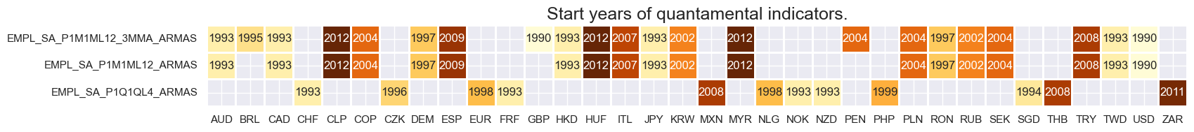
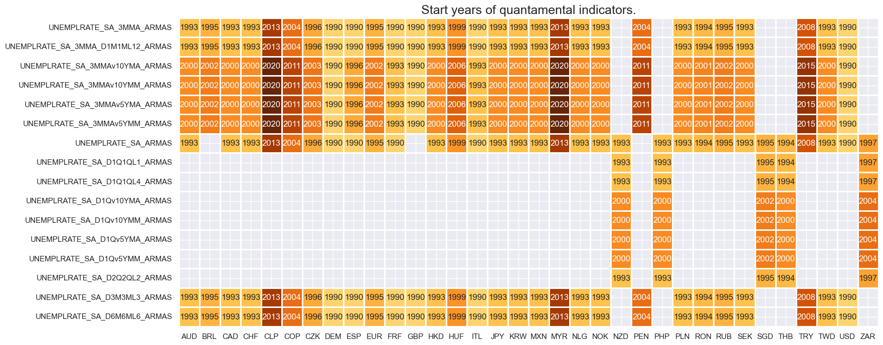
Availability

Availability of real-time quantamental indicators of labor market dynamics, either quarterly or monthly, is very diverse, with some series’ going back to the 1970s and others only starting in the 2010s.

For the explanation of currency symbols, which are related to currency areas or countries for which categories are available, please view Appendix 1 .

xcatx = xcats_empl
cidx = cids_lab

msm.check_availability(
    df,
    xcats=xcatx,
    cids=cidx,
    missing_recent=False,
)

xcatx = xcats_unempl
cidx = cids_lab

msm.check_availability(
    df,
    xcats=xcatx,
    cids=cidx,
    missing_recent=False,
)

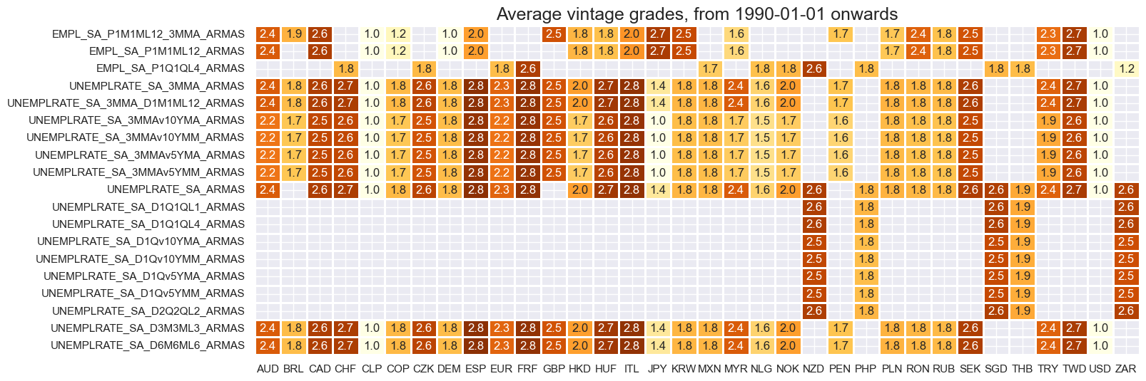
xcatx = xcats_empl + xcats_unempl
cidx = cids_lab

plot = msp.heatmap_grades(
    df,
    xcats=xcatx,
    cids=cidx,
    start=start_date,
    size=(16, 6),
    title=f"Average vintage grades, from {start_date} onwards",
)

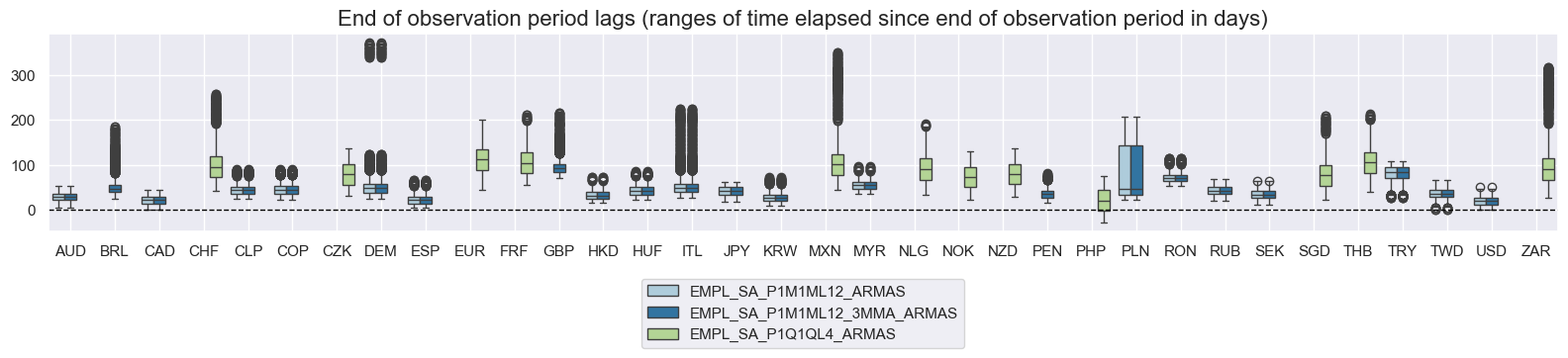
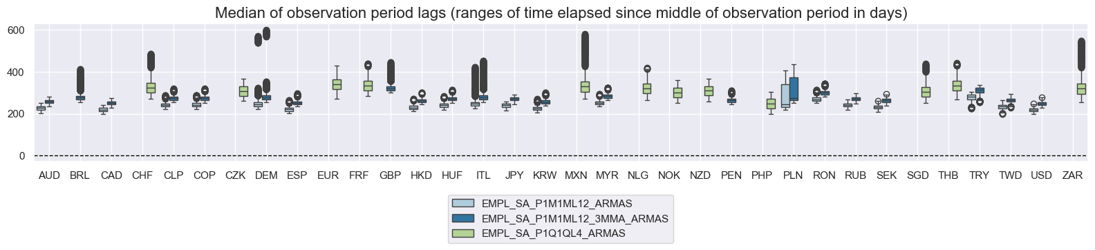
Most employment indicators maintain consistent publication schedules; however, certain cross-sections have experienced extended periods without new releases. Notably, DEM exhibited higher end-of-period lags in 1999 and 2000, but since 2006 these lags have consistently remained below 70 days. MXN experienced an exceptional publication delay in 2020 and 2021, attributable to the COVID-19 pandemic.

xcatx = ["EMPL_SA_P1M1ML12_ARMAS", "EMPL_SA_P1M1ML12_3MMA_ARMAS", "EMPL_SA_P1Q1QL4_ARMAS"]
cidx = cids_lab
msp.view_ranges(
    df,
    xcats=xcatx,
    cids=cidx,
    val="eop_lag",
    title="End of observation period lags (ranges of time elapsed since end of observation period in days)",
    start="2000-01-01",
    kind="box",
    size=(16, 4),
)
msp.view_ranges(
    df,
    xcats=xcatx,
    cids=cidx,
    val="mop_lag",
    title="Median of observation period lags (ranges of time elapsed since middle of observation period in days)",
    start="2000-01-01",
    kind="box",
    size=(16, 4),
)

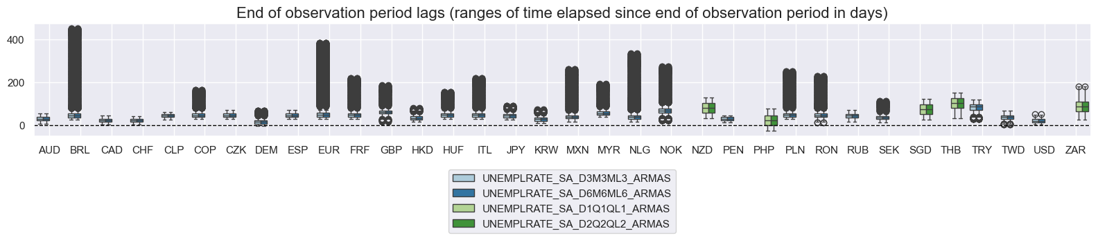
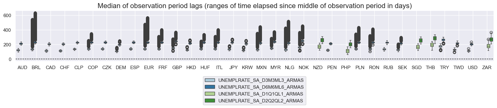
Similar trends apply to unemployment rate indicators. For EUR, the eop_lag has remained constant at 70 days since 2002. GBP saw an extended gap in data releases from September 2023 to February 2024, due to widely reported unreliability in data produced by the Office for National Statistics during this period.

xcatx = [
    "UNEMPLRATE_SA_D3M3ML3_ARMAS",
    "UNEMPLRATE_SA_D6M6ML6_ARMAS",
    "UNEMPLRATE_SA_D1Q1QL1_ARMAS",
    "UNEMPLRATE_SA_D2Q2QL2_ARMAS",
]
cidx = cids_lab
msp.view_ranges(
    df,
    xcats=xcatx,
    cids=cidx,
    val="eop_lag",
    title="End of observation period lags (ranges of time elapsed since end of observation period in days)",
    start="2000-01-01",
    kind="box",
    size=(16, 4),
)
msp.view_ranges(
    df,
    xcats=xcatx,
    cids= cidx,
    val="mop_lag",
    title="Median of observation period lags (ranges of time elapsed since middle of observation period in days)",
    start="2000-01-01",
    kind="box",
    size=(16, 4),
)

For the purpose of the below presentation, we have renamed quarterly-frequency indicators to approximate monthly equivalents in order to have a full panel of similar measures across most countries. The two series’ are not identical but are close substitutes.

quarterly_empl_cids = (
    dfx[dfx["xcat"].isin(main) & dfx["xcat"].str.contains("Q") & dfx["xcat"].str.startswith("EMPL")]
    [["cid", "xcat"]].drop_duplicates()["cid"].tolist()
)

quarterly_unempl_cids = (
    dfx[dfx["xcat"].isin(main) & dfx["xcat"].str.contains("Q") & dfx["xcat"].str.startswith("UNEMPL")]
    [["cid", "xcat"]].drop_duplicates()["cid"].tolist()
)

dict_repl = {
    'EMPL_SA_P1Q1QL4_ARMAS': 'EMPL_SA_P1M1ML12_3MMA_ARMAS',
    'UNEMPLRATE_SA_D1Q1QL4_ARMAS': 'UNEMPLRATE_SA_3MMA_D1M1ML12_ARMAS',
    'UNEMPLRATE_SA_D1Q1QL1_ARMAS': 'UNEMPLRATE_SA_D3M3ML3_ARMAS',
    'UNEMPLRATE_SA_D2Q2QL2_ARMAS': 'UNEMPLRATE_SA_D6M6ML6_ARMAS',
    'UNEMPLRATE_SA_ARMAS' : 'UNEMPLRATE_SA_3MMA_ARMAS',
    'UNEMPLRATE_SA_D1Qv5YMA_ARMAS': 'UNEMPLRATE_SA_3MMAv5YMA_ARMAS',
    'UNEMPLRATE_SA_D1Qv5YMM_ARMAS': 'UNEMPLRATE_SA_3MMAv5YMM_ARMAS',
    'UNEMPLRATE_SA_D1Qv10YMA_ARMAS': 'UNEMPLRATE_SA_3MMAv10YMA_ARMAS',
    'UNEMPLRATE_SA_D1Qv10YMM_ARMAS': 'UNEMPLRATE_SA_3MMAv10YMM_ARMAS',
}

for k, v in dict_repl.items():
    if k.startswith("EMPL"):
        mask = dfx["cid"].isin(quarterly_empl_cids) & dfx["xcat"].str.contains(k)
    elif k.startswith("UNEMPL"):
        mask = dfx["cid"].isin(quarterly_unempl_cids) & dfx["xcat"].str.contains(k)

    dfx.loc[mask, "xcat"] = dfx.loc[mask, "xcat"].str.replace(k, v)

History

Employment growth surprises

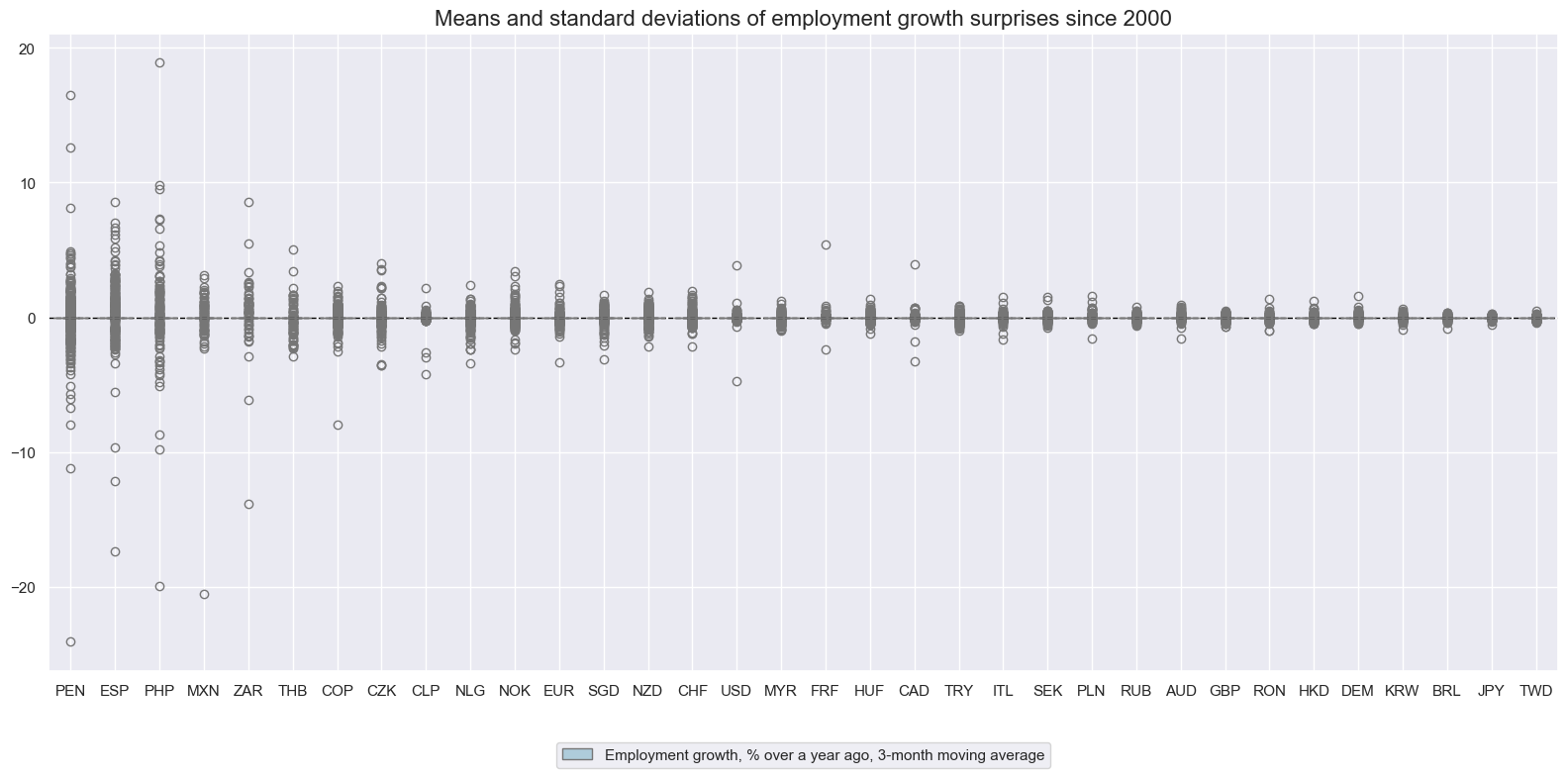
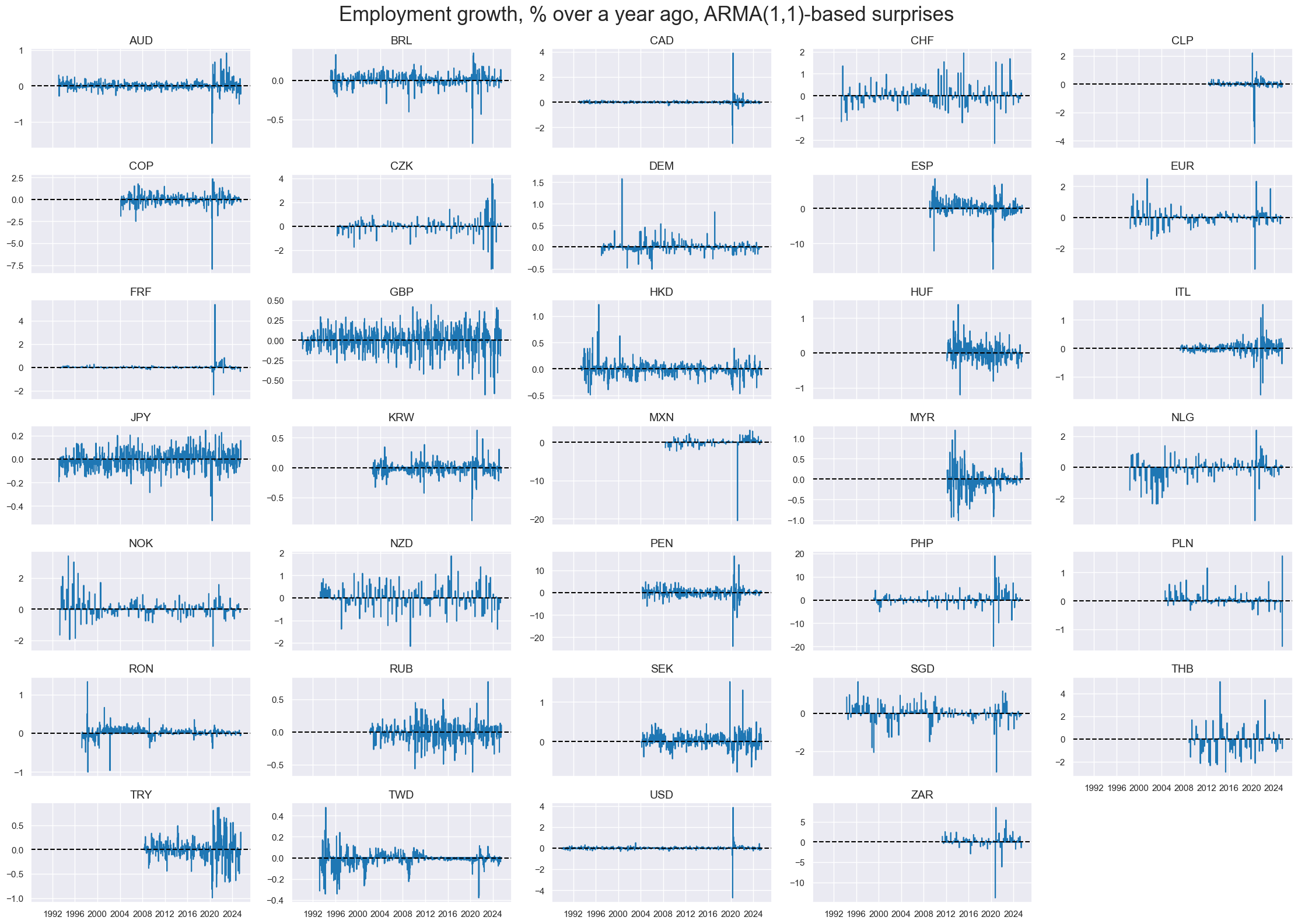
As for other indicators, employment growth surprises are close to white noise, with little autocorrelation. They also show a proclivity to outliers and great variations in standard deviations and across time. This points to the need of some normalization and winsorization of related signals if the surprises are used as indications for the overall economy.

cidx = sorted(cids_lab)
xcatx = ["EMPL_SA_P1M1ML12_3MMA_ARMAS"]

msp.view_ranges(
    dfx,
    xcats=xcatx,
    cids=cidx,
    sort_cids_by="std",
    start=start_date,
    kind="box",
    size=(16, 8),
    title="Means and standard deviations of employment growth surprises since 2000",
    xcat_labels=["Employment growth, % over a year ago, 3-month moving average"],
)

cidx = sorted(cids_lab)
xcatx = ["EMPL_SA_P1M1ML12_3MMA_ARMAS"]

msp.view_timelines(
    dfx,
    xcats=xcatx,
    cids=cidx,
    start=start_date,
    title="Employment growth, % over a year ago, ARMA(1,1)-based surprises",
    xcat_labels= ["3-month moving average"],
    ncol=5,
    aspect=2,
    height=1.5,
    same_y=False,
    legend_fontsize=20,
    title_fontsize=25,
    size=(12, 7),
    all_xticks=False,
)

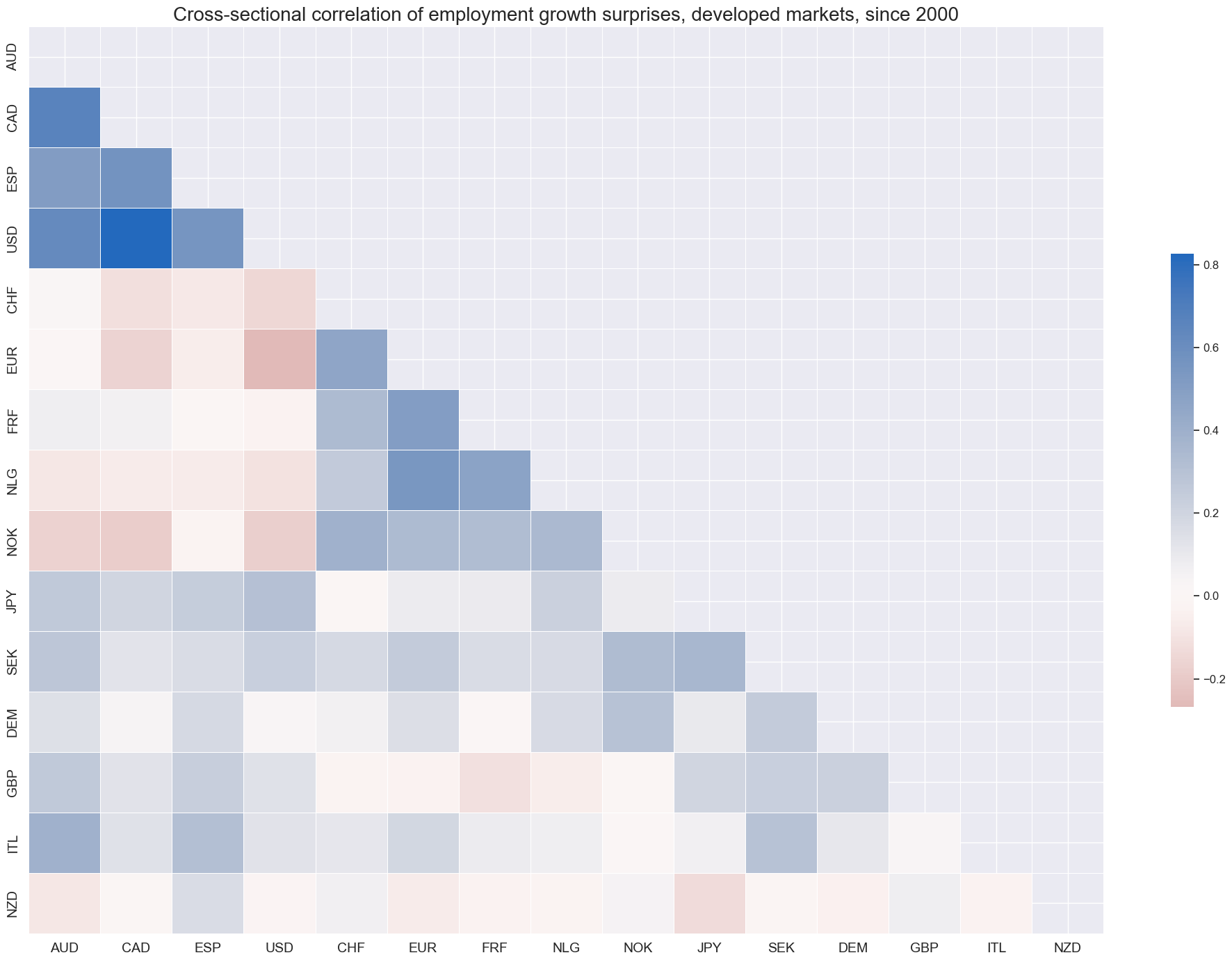
Employment growth surprises are not uniformly positively correlated, even in quarterly averages, suggesting that they may be suitable as components of country-specific signals in a diversified portfolio.

msp.correl_matrix(
    dfx,
    xcats="EMPL_SA_P1M1ML12_3MMA_ARMAS",
    cids=cids_dm,
    start="2000-01-01",
    title="Cross-sectional correlation of employment growth surprises, developed markets, since 2000",
    freq="q",
    cluster=True,
    size=(20, 14),
)

Surprises in annual changes in unemployment rates

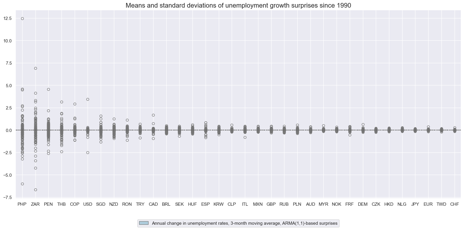
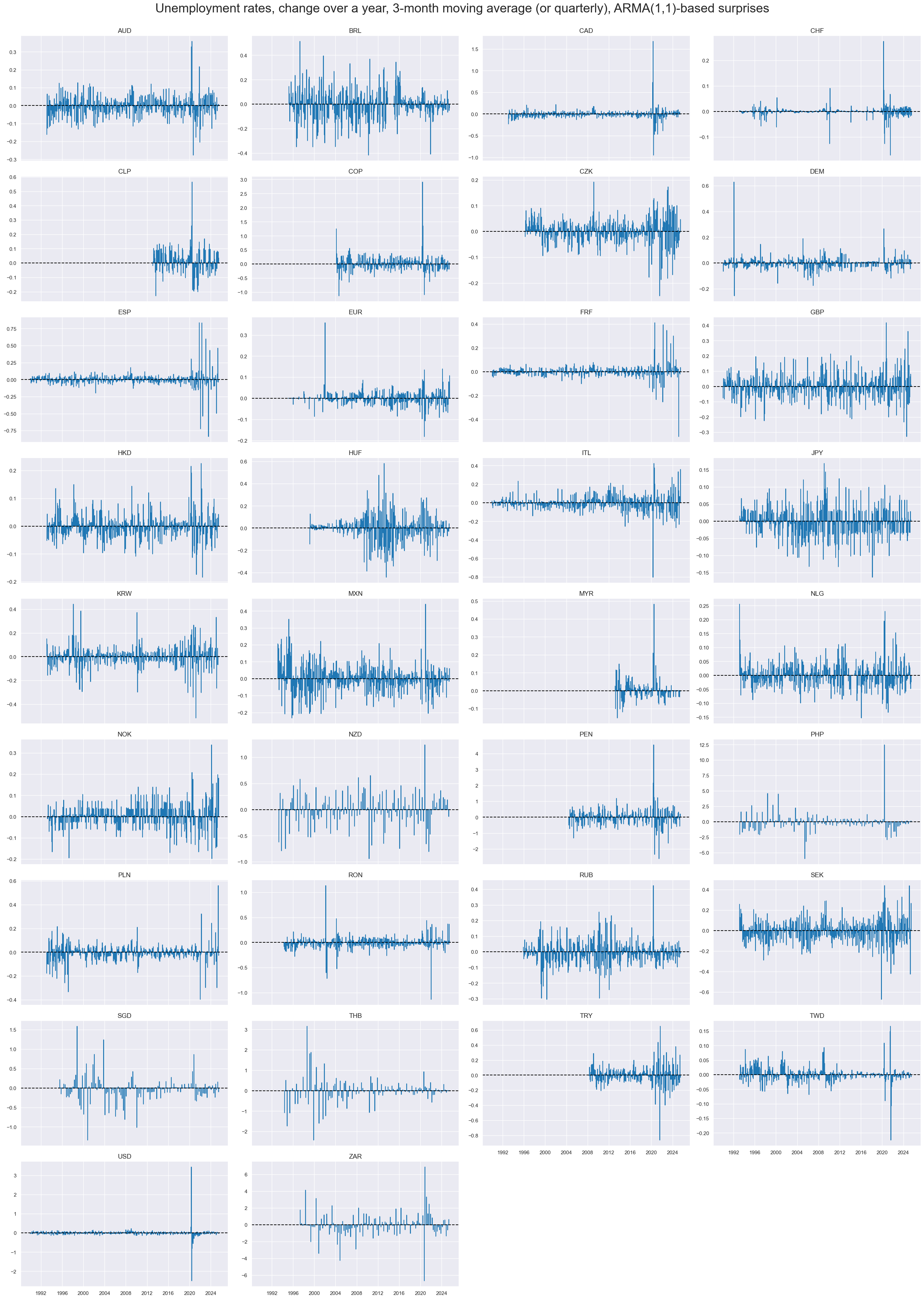
Volatility of unemployment rate changes have been very different across countries, reflecting differences in labor markets and social security incentives for registration, as well as the general registered level of joblessness.

xcatx = ["UNEMPLRATE_SA_3MMA_D1M1ML12_ARMAS"]
cidx = list(set(cids_lab))

msp.view_ranges(
    dfx,
    xcats=xcatx,
    cids=cidx,
    sort_cids_by="std",
    start=start_date,
    title="Means and standard deviations of unemployment growth surprises since 1990",
    xcat_labels=["Annual change in unemployment rates, 3-month moving average, ARMA(1,1)-based surprises"],
    kind="box",
    size=(16, 8),
)

xcatx = ["UNEMPLRATE_SA_3MMA_D1M1ML12_ARMAS"]
cidx = sorted(list(set(cids_lab)))

msp.view_timelines(
    dfx,
    xcats=xcatx,
    cids=cidx,
    start=start_date,
    title="Unemployment rates, change over a year, 3-month moving average (or quarterly), ARMA(1,1)-based surprises",
    legend_fontsize=17,
    title_fontsize=27,
    ncol=4,
    same_y=False,
    size=(12, 7),
    all_xticks=False,
)

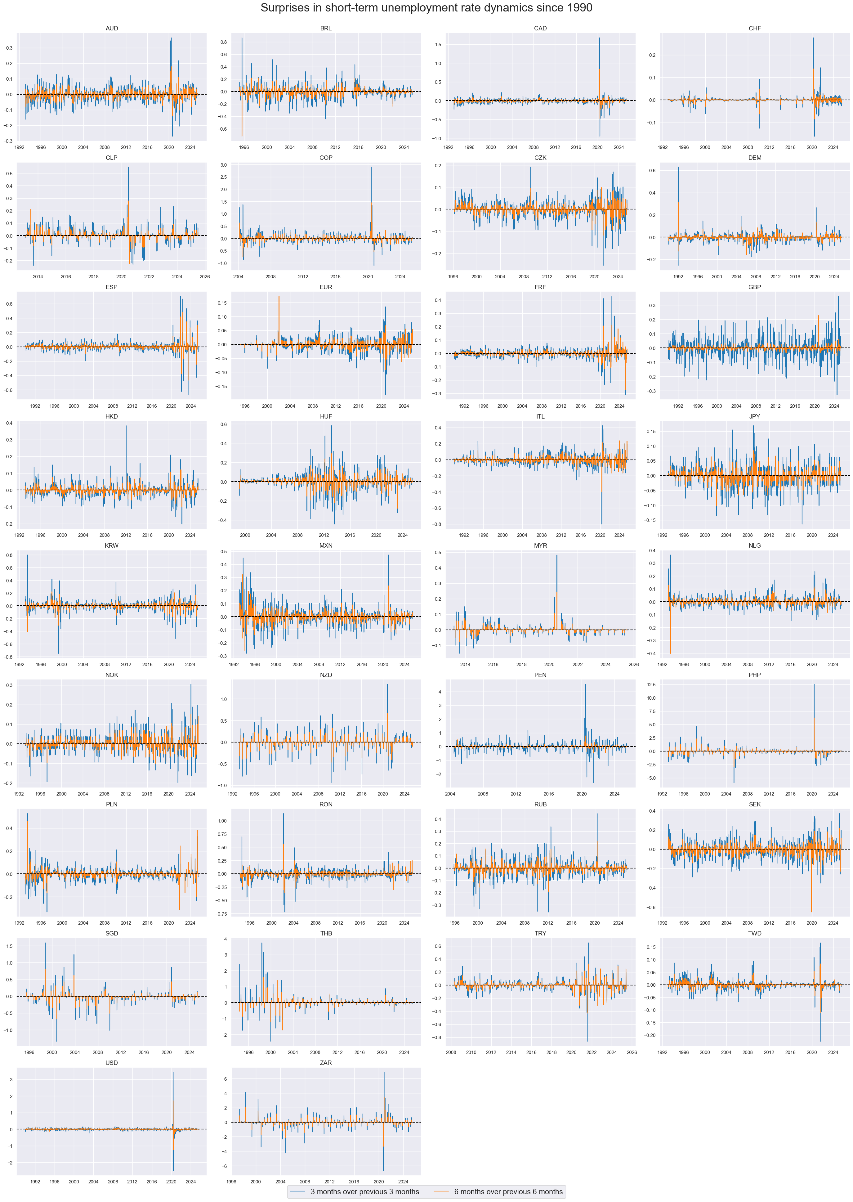
Surprises in shorter-term unemployment rates changes

Surprises look much like white noise, whicht heteroskedasticity across time and countries.

xcatx = ["UNEMPLRATE_SA_D3M3ML3_ARMAS", "UNEMPLRATE_SA_D6M6ML6_ARMAS"]
cidx = cids_lab
msp.view_timelines(
    dfx,
    xcats=xcatx,
    cids=cidx,
    start=start_date,
    title="Surprises in short-term unemployment rate dynamics since 1990",
    xcat_labels=["3 months over previous 3 months", "6 months over previous 6 months"],
    legend_fontsize=17,
    title_fontsize=27,
    ncol=4,
    same_y=False,
    size=(12, 7),
    all_xticks=True,
)

msp.correl_matrix(
    dfx, 
    xcats="UNEMPLRATE_SA_D6M6ML6_ARMAS", 
    cids=cids_dm, 
    size=(20, 14),
    freq="q",
    title="Cross-sectional correlation of unemployment rate surprises, developed markets, since 2000",
    start="2000-01-01",
)

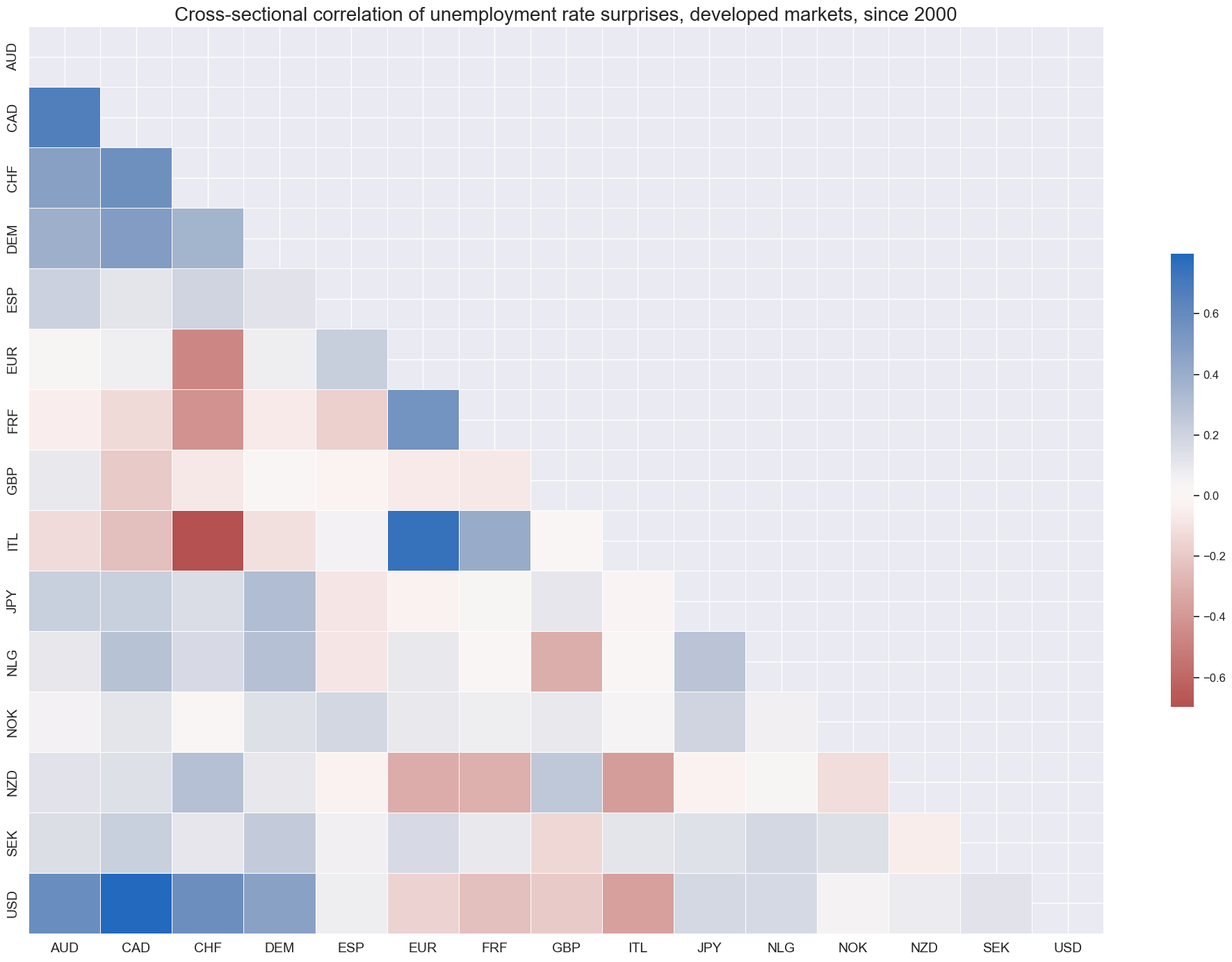
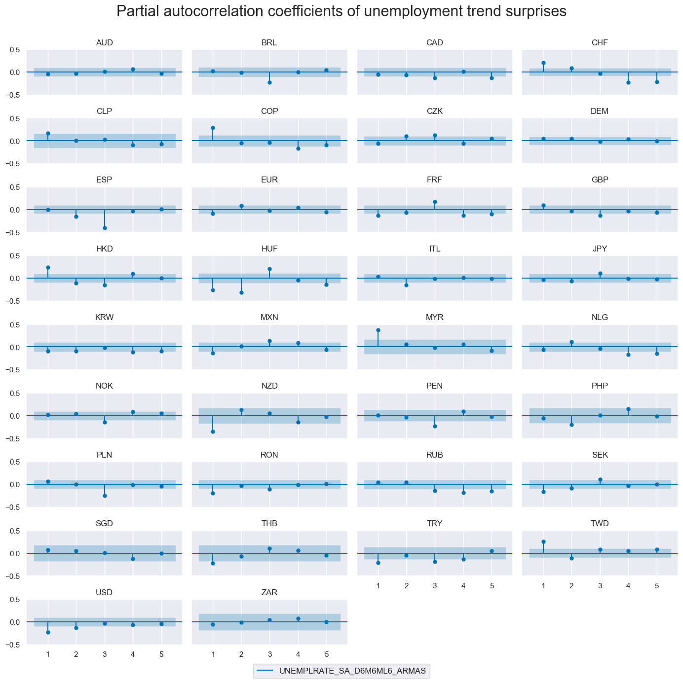
There has been positive or negative autocorrelation in unemployment rate changes across countries, with some countries showing a tendency for unemployment rate changes to revert to the mean, while others show a tendency for unemployment rate changes to persist.

msv.plot_pacf(
    df=dfx,
    cids=cidx,
    xcat="UNEMPLRATE_SA_D6M6ML6_ARMAS",
    title="Partial autocorrelation coefficients of unemployment trend surprises",
    lags=5,
    remove_zero_predictor=True,
    figsize=(14, 14),
    ncols=4,
)

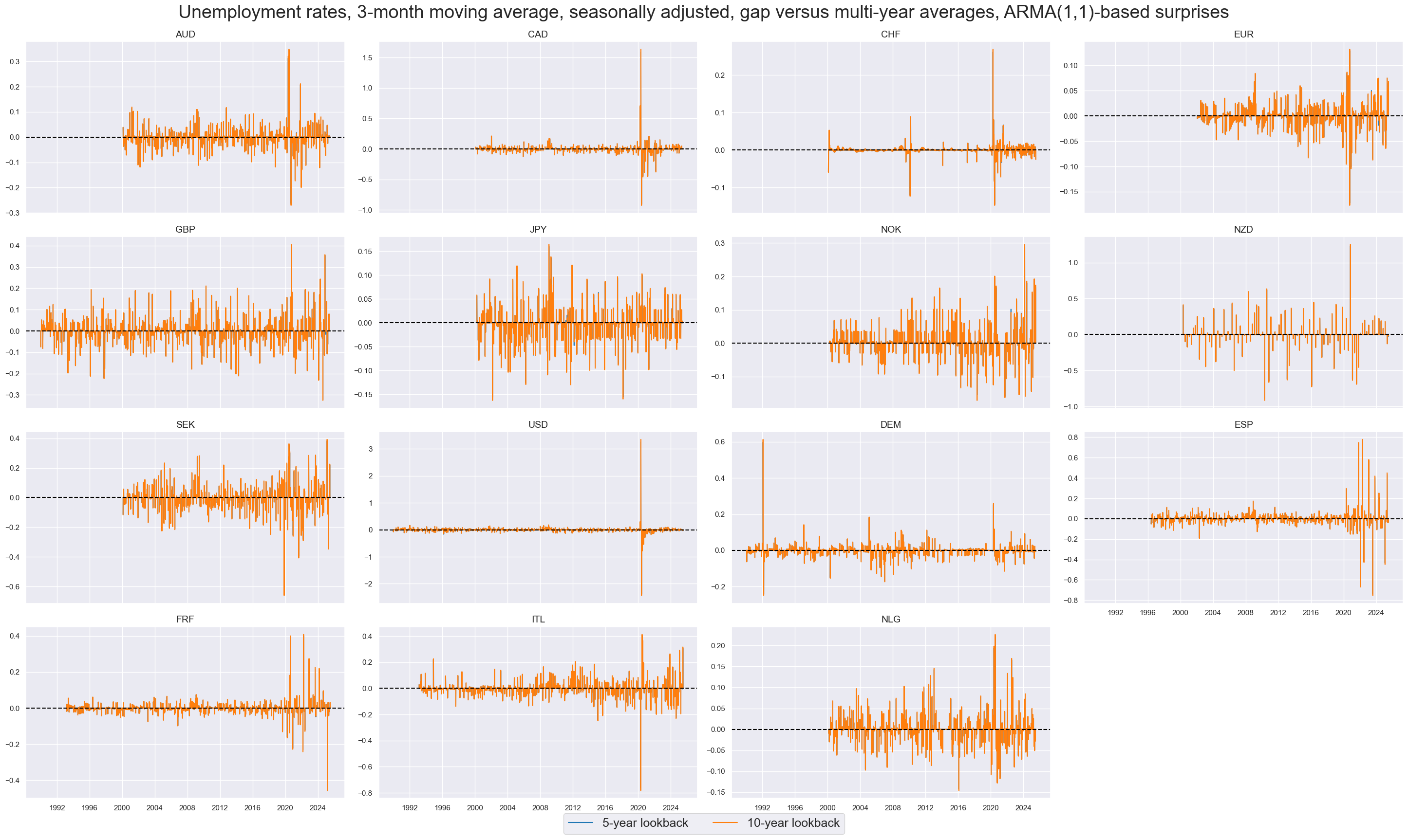
Surprises in unemployment rate gaps (vs 5-10y averages)

xcatx = ["UNEMPLRATE_SA_3MMAv5YMA_ARMAS", "UNEMPLRATE_SA_3MMAv10YMA_ARMAS"]
cidx = cids_dm

msp.view_timelines(
    dfx,
    xcats=xcatx,
    cids=cidx,
    start=start_date,
    title="Unemployment rates, 3-month moving average, seasonally adjusted, gap versus multi-year averages, ARMA(1,1)-based surprises",
    xcat_labels=["5-year lookback", "10-year lookback"],
    legend_fontsize=18,
    title_fontsize=27,
    ncol=4,
    same_y=False,
    size=(12, 7),
    aspect=1.7,
    all_xticks=False,
)

Importance

Research links

• Equity Returns, Unemployment, and Monetary Policy (2020)
  Yijie Li and Matti Suominen
  “We investigate both theoretically and empirically how unemployment level and its growth affect future stock returns. We find that both a higher unemployment rate and higher growth of unemployment positively predict future stock market returns.We investigate both theoretically and empirically how unemployment level and its growth affect future stock returns. We find that both a higher unemployment rate and higher growth of unemployment positively predict future stock market returns.”

• The stock market’s reaction to unemployment news, stock-bond return correlations, and the state of the economy (2006)
  John H. Boyd, Ravi Jagannathanb, and Qianqiu Liuc
  “…on average, the stock market responds positively to news of rising unemployment in expansions, and negatively in contractions. It follows that, since the economy is usually in an expansion phase, the stock market usually rises on bad labor market news.”

• The Reaction of Interest Rates to the Employment Report: The Role of Policy Anticipations (2012)
  Timothy Cook and Steven Korn
  “Interest rates have reacted strongly to the monthly employment report in recent years…The reaction of rates to the report and provide evidence that it has been stronger since the mid-1980s than in earlier years. Evidently the report now has greater impact…on expectations of where the Fed is going to move the federal funds rate. These expectations influence longer-term money market rates.”

Empirical clues

# Normalization and winsorization of employment growth surprises

xcatx = ["EMPL_SA_P1M1ML12_3MMA_ARMAS"]
cidx = cids
df_red = msm.reduce_df(dfx, xcats=xcatx, cids=cidx)

isc_obj = msm.InformationStateChanges.from_qdf(
    df=df_red,
    norm=True,
    std="std",
    min_periods=36,
    score_by="level"
)
dfa = isc_obj.to_qdf(value_column="zscore", postfix="N", thresh=3)

dfc = msm.update_df(dfx, dfa[["real_date", "cid", "xcat", "value"]])

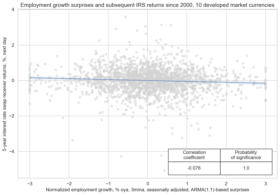
Labor market dynamics have great influence of expected monetary policy. Generally, downside surprises in employment and upside surprises in unemployment translate into a shift of expectations towards a more dovish monetary policy stance, which is a positive “shock” for duration exposure.

In accordance with this relation and the assumption of slight delays in the pricing of new information, we have found that employment growth surprises have been significant negative predictors for next day duration returns, as indicated by 5-year IRS fixed receiver returns. The relation is time sensitive, however, and the surprise effect loses its predictive power after a few days.

cr = msp.CategoryRelations(
    dfc,
    xcats=["EMPL_SA_P1M1ML12_3MMA_ARMASN", "DU05YXR_VT10"],
    cids=cids_dmca,
    freq="D",
    lag=1,
    xcat_aggs=["mean", "sum"],
    fwin=1,
    start="2000-01-01",
    years=None,
    xcat_trims=[None, 8],
)

cr.reg_scatter(
    coef_box="lower right",
    title="Employment growth surprises and subsequent IRS returns since 2000, 10 developed market currencies",
    xlab="Normalized employment growth, % oya, 3mma, seasonally adjusted, ARMA(1,1)-based surprises",
    ylab="5-year interest rate swap receiver returns, %, next day",
    prob_est="map",
    remove_zero_predictor=True,
    size=(10, 7)
)

# Normalization and winsorization of unemployment rate surprises

xcatx = ["UNEMPLRATE_SA_ARMAS", "UNEMPLRATE_SA_D6M6ML6_ARMAS"]
cidx = cids_dmca
df_red = msm.reduce_df(dfx, xcats=xcatx, cids=cidx)

isc_obj = msm.InformationStateChanges.from_qdf(
    df=df_red,
    norm=True,
    std="std",
    min_periods=36,
    score_by="level"
)
dfa = isc_obj.to_qdf(value_column="zscore", postfix="N", thresh=3)

dfc = msm.update_df(dfx, dfa[["real_date", "cid", "xcat", "value"]])

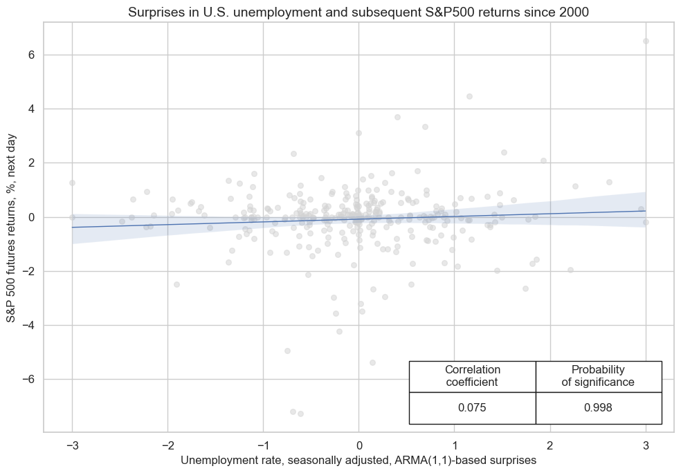
In the U.S., upside surprises to the unemployment rate have positively and significantly predicted next-day equity index returns. Since the U.S. has a central bank with an employment objective and a very flexible labor market, higher-than-expected unemployment typically translates into more-than-expected monetary policy support and less labor cost pressure.

cr = msp.CategoryRelations(
    dfc,
    xcats=["UNEMPLRATE_SA_ARMASN", "EQXR_NSA"],
    cids=["USD"],
    freq="D",
    lag=1,
    xcat_aggs=["sum", "sum"],
    fwin=1,
    start="2000-01-01",
    years=None,
    # xcat_trims=[None, 8],
)

cr.reg_scatter(
    coef_box="lower right",
    title="Surprises in U.S. unemployment and subsequent S&P500 returns since 2000",
    xlab="Unemployment rate, seasonally adjusted, ARMA(1,1)-based surprises",
    ylab="S&P 500 futures returns, %, next day",
    prob_est="map",
    remove_zero_predictor=True,
    size=(10, 7)
)

Appendices

Appendix 1: Currency symbols

The word ‘cross-section’ refers to currencies, currency areas or economic areas. In alphabetical order, these are AUD (Australian dollar), BRL (Brazilian real), CAD (Canadian dollar), CHF (Swiss franc), CLP (Chilean peso), CNY (Chinese yuan renminbi), COP (Colombian peso), CZK (Czech Republic koruna), DEM (German mark), ESP (Spanish peseta), EUR (Euro), FRF (French franc), GBP (British pound), HKD (Hong Kong dollar), HUF (Hungarian forint), IDR (Indonesian rupiah), ITL (Italian lira), JPY (Japanese yen), KRW (Korean won), MXN (Mexican peso), MYR (Malaysian ringgit), NLG (Dutch guilder), NOK (Norwegian krone), NZD (New Zealand dollar), PEN (Peruvian sol), PHP (Phillipine peso), PLN (Polish zloty), RON (Romanian leu), RUB (Russian ruble), SEK (Swedish krona), SGD (Singaporean dollar), THB (Thai baht), TRY (Turkish lira), TWD (Taiwanese dollar), USD (U.S. dollar), ZAR (South African rand).

Appendix 2: Quantamental economic surprises

Quantamental economic surprises are defined as deviations of point-in-time quantamental indicators from expected values. Expected values are estimated predictions of an informed market participant. Following this definition there are two types of surprises that jointly make up economic surprise indicators:

• A first print event is the difference between a quantamental indicator on a release date and its expected value. A release date is the day on which any underlying economic time series adds an observation period. Expected values are estimated, typically based on econometric models and information prior to the release date. A quantamental data surprise is always specific to the prediction model or statistical learning process.

• A pure revision event is the change in a quantamental indicator on a non-release date. It arises from revisions of data for previously released observation periods. Per default, it is assumed that all revisions are surprises, i.e., that the latest reported value for an observation period is the best predictor its value after revisions. Note that any revisions published on a release date become part of the first print event.

A quantamental indicator of economic surprises records the values of these two events on the dates they become known. It records zero values for all other dates. Models for predicting indicator values always use the latest vintage of the underlying data series. They are typically applied to increments, i.e., differences or log differences of volume, value or price indices. The predicted next increment produces an expected new vintage, and the expected new vintage implies a new derived expected quantamental indicator, such as an annual growth rate or moving average. Note than in this way predictions automatically account for “base effects”, i.e., predictable changes in growth rates that arise from unusually sharp increase of declines in index levels of the base period, for example a year ago.