Consumer price inflation surprises

This category contains economic surprise indicators related to consumer price inflation growth trends . These indicators measure the difference between realised inflation data and model-implied expectations formed using only information available before the release — a proxy for what the market might reasonably have expected at the time. They provide a systematic view of inflation surprises, defined as deviations from credible real-time forecasts.

For detailed methodology on surprise construction, including transformation logic and real-time forecast design, see Appendix 2 and the research article Quantamental economic surprise indicators: a primer .

Annual CPI inflation surprises

Ticker : CPIH_SA_P1M1ML12_ARMAS / CPIC_SA_P1M1ML12_ARMAS / CPIXFE_SA_P1M1ML12_ARMAS

Label : ARMA(1,1)-based surprises: Headline CPI inflation, % oya / Core CPI inflation, % oya / Consistent core CPI inflation, % oya

Definition : ARMA(1,1)-based surprises: Headline CPI inflation, % over a year ago / Core CPI inflation, % over a year ago / Consistent core CPI inflation, % over a year ago

Notes :

• Refer to the section on consumer price inflation growth trends and consistent core consumer price inflation trends for details on the underlying data series.

• Expected values are derived from the one-step-ahead forecast produced by the previous vintage of a univariate ARMA(1,1) time series model. This model predicts monthly log-changes of the price index, based on the previous month’s value (autoregressive component) and the most recent model residual (i.e. the in-sample error used in the moving average component). These forecasts are applied to the price index to construct the expected year-over-year inflation rate.

• Model coefficients are estimated separately for each data vintage, using only the information available at that point in time. This ensures every forecast is genuinely out-of-sample, reflecting expectations based on real-time data.

• Surprises are calculated as the difference between the actual and forecasted value of the year-over-year percentage change in the relevant consumer price index. In the case of pure revisions, without release of a new observation period, the surprise is the difference between the pre-release and post-release inflation rate.

Short-term (% 3m/3m) CPI inflation surprises

Ticker : CPIH_SJA_P3M3ML3AR_ARMAS / CPIC_SJA_P3M3ML3AR_ARMAS / CPIXFE_SJA_P3M3ML3AR_ARMAS

Label : ARMA(1,1)-based surprises: Headline CPI inflation, % 3m/3m, saar / Core CPI inflation, % 3m/3m, saar / Consistent core CPI inflation, % 3m/3m, saar

Definition : ARMA(1,1)-based surprises: Headline CPI inflation, % 3 months over previous 3 months, seasonally-adjusted annualized rate / Core CPI inflation, % 3 months over previous 3 months, seasonally-adjusted annualized rate / Consistent core CPI inflation, % 3 months over previous 3 months, seasonally-adjusted annualized rate

Notes :

• Refer to the section on consumer price trends and consistent core consumer price inflation trends for details on the underlying data series.

• Expected values are derived from the one-step-ahead forecast produced by the previous vintage of a univariate ARMA(1,1) time series model. This model predicts monthly log-changes of the price index, based on the previous month’s value (autoregressive component) and the most recent model residual (i.e. the in-sample error used in the moving average component). These forecasts are applied to the price index to construct the expected annualised 3m/3m inflation trend.

• Model coefficients are estimated separately for each data vintage, using only the information available at that point in time. This ensures every forecast is genuinely out-of-sample, reflecting expectations based on real-time data.

• Surprises are calculated as the difference between the actual and forecasted value of the percentage change in the relevant consumer price index. In the case of pure revisions, without release of a new observation period, the surprise is the difference between the pre-release and post-release inflation rate.

Short-term (% 6m/6m) CPI inflation surprises

Ticker : CPIH_SJA_P6M6ML6AR_ARMAS / CPIC_SJA_P6M6ML6AR_ARMAS / CPIXFE_SJA_P6M6ML6AR_ARMAS

Label : ARMA(1,1)-based surprises: Headline CPI inflation, % 6m/6m, saar / Core CPI inflation, % 6m/6m, saar / Consistent core CPI inflation, % 6m/6m, saar

Definition : ARMA(1,1)-based surprises: Headline CPI inflation, % 6 months over previous 6 months, seasonally-adjusted annualized rate / Core CPI inflation, % 6 months over previous 6 months, seasonally-adjusted annualized rate / Consistent core CPI inflation, % 6 months over previous 6 months, seasonally-adjusted annualized rate

Notes :

• See notes for the 3m/3m ARMA-based inflation surprises (such as CPIH_SJA_P3M3ML3AR_ARMAS ) for model specification and methodology. The only difference lies in the transformation, i.e., the annualised 6-month-over-6-month change in prices.

Monthly CPI change surprises

Ticker : CPIH_SJA_P1M1ML1_ARMAS / CPIC_SJA_P1M1ML1_ARMAS / CPIXFE_SJA_P1M1ML1_ARMAS

Label : ARMA(1,1)-based surprises: Headline CPI inflation, %m/m / Core CPI inflation, %m/m / Consistent core CPI inflation, %m/m

Definition : ARMA(1,1)-based surprises: Headline CPI inflation, % month on month / Core CPI inflation, % month on month / Consistent core CPI inflation, % month on month

Notes :

• See notes for the 3m/3m ARMA-based inflation surprises (such as CPIH_SJA_P3M3ML3AR_ARMAS ) for model specification and methodology. The only difference lies in the transformation, which here reflects the one-month-over-one-month change in adjusted consumer prices.

CPI inflation change surprises

Ticker : CPIH_SJA_P1M1ML12_D1M1ML3_ARMAS / CPIC_SJA_P1M1ML12_D1M1ML3_ARMAS / CPIXFE_SJA_P1M1ML12_D1M1ML3_ARMAS

Label : ARMA(1,1)-based surprises: Headline CPI inflation, %oya, diff over 3m / Core CPI inflation, %oya, diff over 3m / Consistent core CPI inflation, %oya, diff over 3m

Definition : ARMA(1,1)-based surprises: Headline CPI inflation, %oya, change over the last 3 months / Core CPI inflation, %oya, change over the last 3 months / Consistent core CPI inflation, %oya, change over the last 3 months

Notes :

• Refer to the section on change in headline consumer price inflation and change in consistent core consumer price inflation for details on the underlying data series.

• Expected values are derived from the one-step-ahead forecast produced by the previous vintage of a univariate ARMA(1,1) time series model. This model predicts monthly log-changes of the price index, based on the previous month’s value (autoregressive component) and the most recent model residual (i.e. the in-sample error used in the moving average component). These forecasts are applied to the price index to construct the expected change in the year-over-year inflation rate relative to three months earlier, within the same release.

• Model coefficients are estimated separately for each data vintage, using only the information available at that point in time. This ensures every forecast is genuinely out-of-sample, reflecting expectations based on real-time data.

• Surprises are calculated as the difference between the actual and forecasted value of the 3-month change in annual inflation in the relevant consumer price index. In the case of pure revisions, without release of a new observation period, the surprise is the difference between the pre-release and post-release inflation rate.

Core CPI changes, using early estimates and ARMAX models

Ticker : CPICE_SA_P1M1ML12_ARMAXS / CPICE_SJA_P3M3ML3AR_ARMAXS / CPICE_SJA_P6M6ML6AR_ARMAXS / CPICE_SA_P1M1ML12_D1M1ML3_ARMAXS

Label : Core CPI, using early estimates, ARMAX(1,1)-based surprises: % oya / % 3m/3m saar (jump-adjusted) / % 6m/6m saar (jump-adjusted) / change in % oya over 3 months

Definition : Core consumer price inflation, using early estimates, ARMAX(1,1)-based surprises: % oya / % 3m/3m saar (jump-adjusted) / % 6m/6m saar (jump-adjusted) / change of % oya over 3 months

Notes :

• These indicators are currently calculated only for Japan (JPY) and the U.S. (USD). See the section on core CPI changes, using early estimates for details on the underlying data. See also Appendix 3 for the methodology behind surprise construction using early predictors.

• Expected values are based on one-step-ahead forecasts from ARMAX(1,1) models estimated using only data available in each historical vintage. These models predict monthly log-changes in the price index using its own past behaviour and a contemporaneous early-released CPI component.

• The forecasted log-changes are used to reconstruct an index-level forecast. The relevant transformation (e.g. year-over-year inflation or a multi-month trend) is then applied to both the actual and forecasted index. The surprise is defined as the difference between these transformed values.

• Model coefficients are estimated separately for each data vintage, ensuring that all forecasts are genuinely out-of-sample and reflect real-time expectations.

Imports

Only the standard Python data science packages and the specialized macrosynergy package are needed.

# Core libraries
import os
import math
import json
import yaml
import warnings

# Scientific computing and plotting
import numpy as np
import pandas as pd
import matplotlib.pyplot as plt
import seaborn as sns

# Date and timing utilities
from timeit import default_timer as timer
from datetime import timedelta, date, datetime

# Macrosynergy package
import macrosynergy.management as msm
import macrosynergy.panel as msp
import macrosynergy.signal as mss
import macrosynergy.pnl as msn
import macrosynergy.visuals as msv
from macrosynergy.download import JPMaQSDownload

# Suppress warnings for cleaner output
warnings.simplefilter("ignore")

The JPMaQS indicators are retrieved using the J.P. Morgan DataQuery API via the macrosynergy package. Tickers are constructed by combining a currency area code ( <cross_section> ) with an indicator category code ( <category> ), forming a string of the form <cross_section>_<category> .

This composite string is embedded within a full DataQuery ticker:

DB(JPMAQS,<cross_section>_<category>,<info>)

where <info> refers to the type of time series data requested. The available options are:

• value : the latest available value of the indicator

• eop_lag : days since the end of the observation period

• mop_lag : days since the mean observation period

• grade : a real-time data quality metric

To download data, instantiate the JPMaQSDownload class from macrosynergy.download , and use the .download(tickers, start_date, metrics) method, where:

• tickers is a list of constructed ticker strings

• start_date is the first collection date to retrieve

• metrics specifies the types of information (e.g. value , grade ) to download

The macrosynergy package makes it easy to retrieve and work with this data in a fully programmatic and repeatable way.

# Cross-sections of interest by region

# Developed market (DM) currency areas
cids_dmca = [
    "AUD", "CAD", "CHF", "EUR", "GBP", "JPY", "NOK", "NZD", "SEK", "USD"
]

# Developed market euro area countries (pre-euro legacy codes)
cids_dmec = ["DEM", "ESP", "FRF", "ITL", "NLG"]

# Emerging market (EM) Latin America
cids_latm = ["BRL", "COP", "CLP", "MXN", "PEN"]

# Emerging market EMEA
cids_emea = ["CZK", "HUF", "ILS", "PLN", "RON", "RUB", "TRY", "ZAR"]

# Emerging market Asia
cids_emas = [
    "CNY",
    # "HKD",  # Excluded from analysis
    "IDR", "INR", "KRW", "MYR", "PHP", "SGD", "THB", "TWD"
]

# Aggregated developed and emerging markets
cids_dm = sorted(cids_dmca + cids_dmec)
cids_em = sorted(cids_latm + cids_emea + cids_emas)

# Final list of cross-sections (sorted)
cids = sorted(cids_dm + cids_em)

# Exported selection for further use
cids_exp = cids

# Quantamental categories of interest

# Core CPI trend surprise indicators (headline, core, and consistent core)
main = []

# Year-over-year inflation and change-in-inflation: headline and core
for base in ["CPIH_SA", "CPIC_SA"]:
    for transform in ("P1M1ML12", "P1Q1QL4", "P1M1ML12_D1M1ML3", "P1Q1QL4_D1Q1QL1"):
        main.append(f"{base}_{transform}_ARMAS")

# Change-in-inflation only: core
for transform in ("P1M1ML12", "P1M1ML12_D1M1ML3"):
    main.append(f"CPIC_SA_{transform}_ARMAS")

# Year-over-year and change-in-inflation: consistent core
for transform in ("P1M1ML12", "P1Q1QL4", "P1M1ML12_D1M1ML3", "P1Q1QL4_D1Q1QL1"):
    main.append(f"CPIXFE_SA_{transform}_ARMAS")

# Multi-month CPI trends (jump-adjusted): headline, core, consistent core
for base in ["CPIH_SJA", "CPIC_SJA", "CPIXFE_SJA"]:
    for transform in ("P1Q1QL1AR", "P2Q2QL2AR", "P3M3ML3AR", "P6M6ML6AR", "P1M1ML1"):
        main.append(f"{base}_{transform}_ARMAS")

# Core CPI early-estimate (ARMAX-based)
for transform in ("P3M3ML3AR", "P6M6ML6AR"):
    main.append(f"CPICE_SJA_{transform}_ARMAXS")

for transform in ("P1M1ML12", "P1M1ML12_D1M1ML3"):
    main.append(f"CPICE_SA_{transform}_ARMAXS")

# Economic context variables
econ = [
    "RIR_NSA",
    "IVAWGT_SA_1YMA",
    "CPIH_SA_P1M1ML12",
    "CPIC_SA_P1M1ML12"
]

# Market-linked context variables
mark = [
    "FXXR_NSA", "FXXR_VT10",
    "DU02YXR_NSA", "DU02YXR_VT10",
    "DU05YXR_NSA", "DU05YXR_VT10",
    "FXUNTRADABLE_NSA", "FXTARGETED_NSA",
    "EQXR_VT10"
]

# Combined list of cross-sectional categories
xcats = main + econ + mark

# Special industry-related commodity data set

# Commodity identifiers (LME base metals)
cids_co = ["ALM", "CPR", "LED", "NIC", "TIN", "ZNC"]

# Cross-sectional categories
xcats_co = ["COXR_VT10", "COXR_NSA"]

# Combined commodity tickers (cross-section + category)
tix_co = [f"{cid}_{xcat}" for cid in cids_co for xcat in xcats_co]

# Download series from J.P. Morgan DataQuery by tickers

start_date = "1990-01-01"

# Combine tickers for macro indicators and commodity overlays
tickers = [f"{cid}_{xcat}" for cid in cids for xcat in xcats] + tix_co
print(f"Maximum possible number of tickers: {len(tickers)}")

# Retrieve DataQuery API credentials from environment variables
client_id = os.getenv("DQ_CLIENT_ID")
client_secret = os.getenv("DQ_CLIENT_SECRET")

# Download data from DataQuery
start = timer()
with JPMaQSDownload(client_id=client_id, client_secret=client_secret) as downloader:
    df = downloader.download(
        tickers=tickers,
        start_date=start_date,
        metrics=["value", "eop_lag", "mop_lag", "grading"],
        suppress_warning=True,
        show_progress=True,
    )
end = timer()

print(f"Download time from DataQuery: {timedelta(seconds=end - start)}")

# Store downloaded DataFrame
dfd = df

Maximum possible number of tickers: 1714
Downloading data from JPMaQS.
Timestamp UTC:  2025-06-21 21:37:16
Connection successful!

Requesting data: 100%|██████████| 328/328 [01:09<00:00,  4.72it/s]
Downloading data: 100%|██████████| 328/328 [06:10<00:00,  1.13s/it]

Some expressions are missing from the downloaded data. Check logger output for complete list.
2640 out of 6560 expressions are missing. To download the catalogue of all available expressions and filter the unavailable expressions, set `get_catalogue=True` in the call to `JPMaQSDownload.download()`.
Download time from DataQuery: 0:08:02.802473

Availability

# Define subset of cross-sections and key indicator categories for availability check

cidx = cids  # Use all cross-sections previously defined

xcatx = [
    "CPIC_SA_P1M1ML12_ARMAS",    # Core CPI, % oya
    "CPIH_SA_P1M1ML12_ARMAS",    # Headline CPI, % oya
    "CPIXFE_SA_P1M1ML12_ARMAS",  # Consistent core CPI, % oya
    "CPIC_SA_P1Q1QL4_ARMAS",     # Core CPI, % qoq ann.
    "CPIH_SA_P1Q1QL4_ARMAS",     # Headline CPI, % qoq ann.
    "CPIXFE_SA_P1Q1QL4_ARMAS",   # Consistent core CPI, % qoq ann.
    "CPICE_SA_P1M1ML12_ARMAXS"   # Core CPI (early est.), % oya
]

# Run availability check on selected indicators and cross-sections
msm.check_availability(
    df=dfd,
    xcats=xcatx,
    cids=cidx,
    missing_recent=False,
)

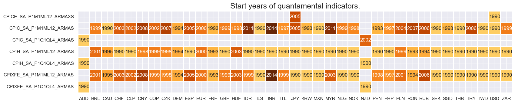
Real-time quantamental indicators of consumer price inflation trends have typically been available for developed markets since the late 1990s. For many emerging markets, data start from around 2000, with headline CPI series often available only later. For an explanation of the currency codes, which refer to currency areas or countries with available categories, see Appendix 1 .

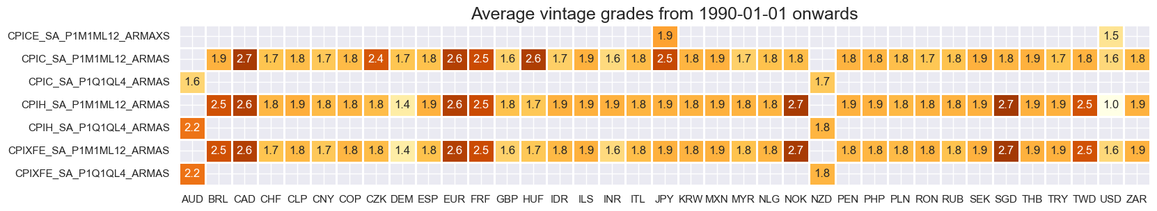
The chart below shows the average vintage grades of core CPI surprise indicators across countries. Grading reflects the timeliness and quality of real-time data available for each series since the start date.

Vintage quality is mixed. USD is the only cross-section with consistently high-grade data extending back to the early 1990s.

xcatx = [
    "CPIC_SA_P1M1ML12_ARMAS",    
    "CPIH_SA_P1M1ML12_ARMAS",     
    "CPIXFE_SA_P1M1ML12_ARMAS",  
    "CPICE_SA_P1M1ML12_ARMAXS", 
    "CPIC_SA_P1Q1QL4_ARMAS",    
    "CPIH_SA_P1Q1QL4_ARMAS",      
    "CPIXFE_SA_P1Q1QL4_ARMAS"    
]

cidx = cids_exp

plot = msp.heatmap_grades(
    dfd,
    xcats=xcatx,
    cids=cidx,
    size=(18, 3),
    title=f"Average vintage grades from {start_date} onwards",
    start=start_date,
)

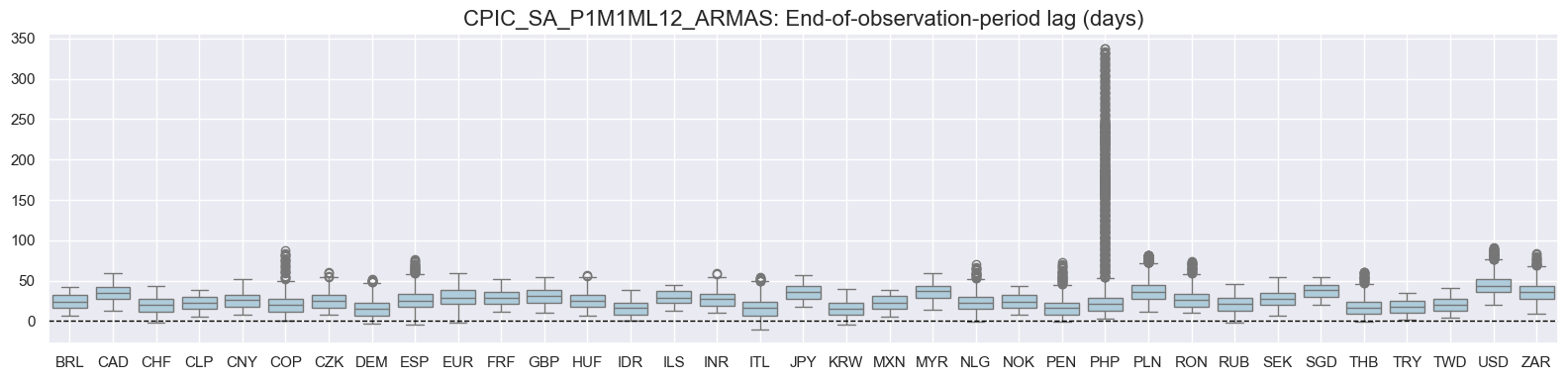
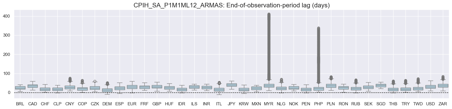
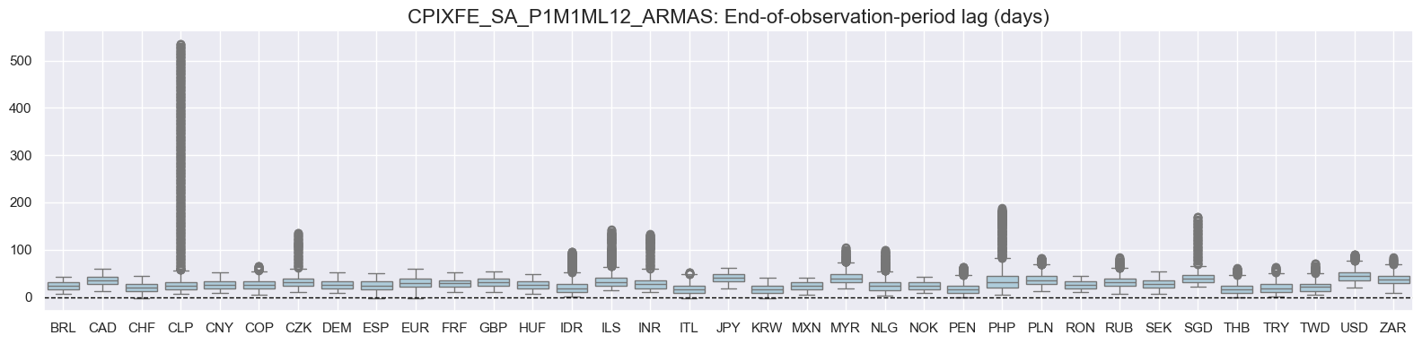
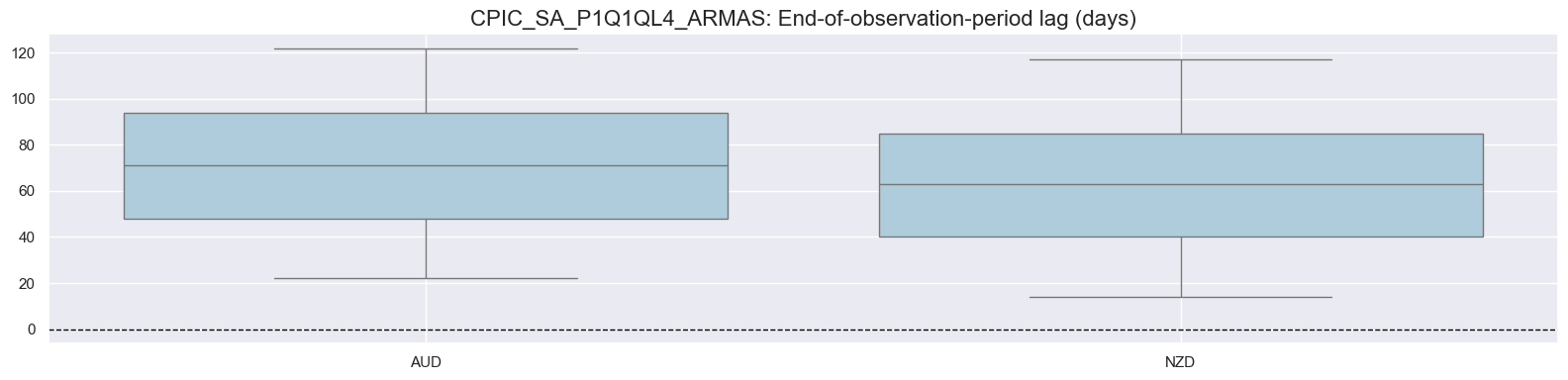
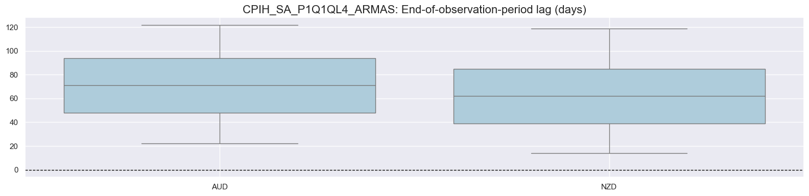
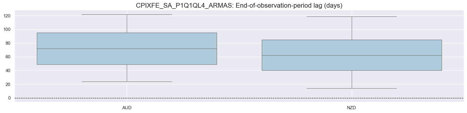
The distribution below shows end-of-observation period lags. US core CPI data experienced one publishing delay due to government shutdowns that affected the release.

# View eop_lag ranges by cross-section for selected CPI surprise indicators

cidx = cids_exp

xcats = [
    "CPIC_SA_P1M1ML12_ARMAS",    
    "CPIH_SA_P1M1ML12_ARMAS",    
    "CPIXFE_SA_P1M1ML12_ARMAS",  
    "CPIC_SA_P1Q1QL4_ARMAS",   
    "CPIH_SA_P1Q1QL4_ARMAS",     
    "CPIXFE_SA_P1Q1QL4_ARMAS",   
]

for xcat in xcats:
    msp.view_ranges(
        dfd,
        xcats=[xcat],
        cids=cidx,
        val="eop_lag",
        title=f"{xcat}: End-of-observation-period lag (days)",
        start=start_date,
        kind="box",
        size=(16, 4),
    )

# Harmonise xcat labels: replace quarterly transformations with equivalent monthly formats

dict_repl = {
    "CPIC_SA_P1Q1QL4_ARMAS": "CPIC_SA_P1M1ML12_ARMAS",
    "CPIH_SA_P1Q1QL4_ARMAS": "CPIH_SA_P1M1ML12_ARMAS",
    "CPIXFE_SA_P1Q1QL4_ARMAS": "CPIXFE_SA_P1M1ML12_ARMAS",
    "CPIH_SJA_P1Q1QL1AR_ARMAS": "CPIH_SJA_P3M3ML3AR_ARMAS",
    "CPIXFE_SJA_P1Q1QL1AR_ARMAS": "CPIXFE_SJA_P3M3ML3AR_ARMAS",
}

# Replace only exact matches for xcat names
dfd["xcat"] = dfd["xcat"].replace(dict_repl)

History

The variance of CPI inflation surprises has been very different across countries and regimes, suggesting a need to scale the surprises by concurrent inflation rates for comparability across countries.

# Boxplots of headline CPI surprise distributions (seasonally adjusted), by country

xcatx = ["CPIH_SA_P1M1ML12_ARMAS"]

# Exclude PEN due to limited data coverage or outlier behaviour
cids_filtered = sorted(set(cids_exp) - {"PEN"})

msp.view_ranges(
    dfd,
    xcats=xcatx,
    cids=cids_filtered,
    sort_cids_by="std",
    start=start_date,
    kind="bar",
    title="Distribution of headline CPI surprises, by country",
    size=(16, 8),
)

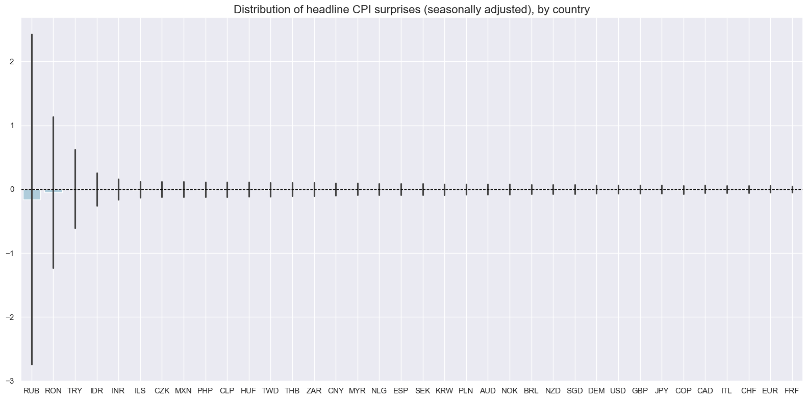
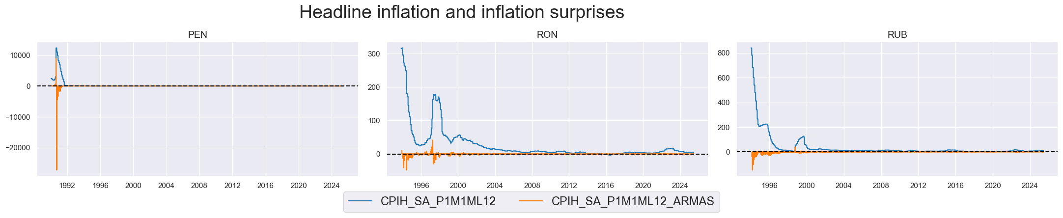
A few countries (Peru, Russia, and Romania) exhibit prolonged periods of non-stationary inflation dynamics. Such periods may invalidate surprise estimates because the ARMA model assumes stationary of time series.

# Timeline plots of headline inflation levels vs. inflation surprises
# Focus on countries with more volatile or non-stationary inflation dynamics

xcatx = [
    "CPIH_SA_P1M1ML12",          # Headline CPI, % oya
    "CPIH_SA_P1M1ML12_ARMAS"     # Surprise in % oya
]

cidx = ["PEN", "RON", "RUB"]

msp.view_timelines(
    dfd,
    xcats=xcatx,
    cids=cidx,
    start=start_date,
    title="Headline inflation and inflation surprises",
    title_adj=1.02,
    title_xadj=0.435,
    title_fontsize=27,
    legend_fontsize=17,
    label_adj=0.075,
    ncol=3,
    same_y=False,
    size=(12, 7),
    aspect=1.7,
    all_xticks=True,
)

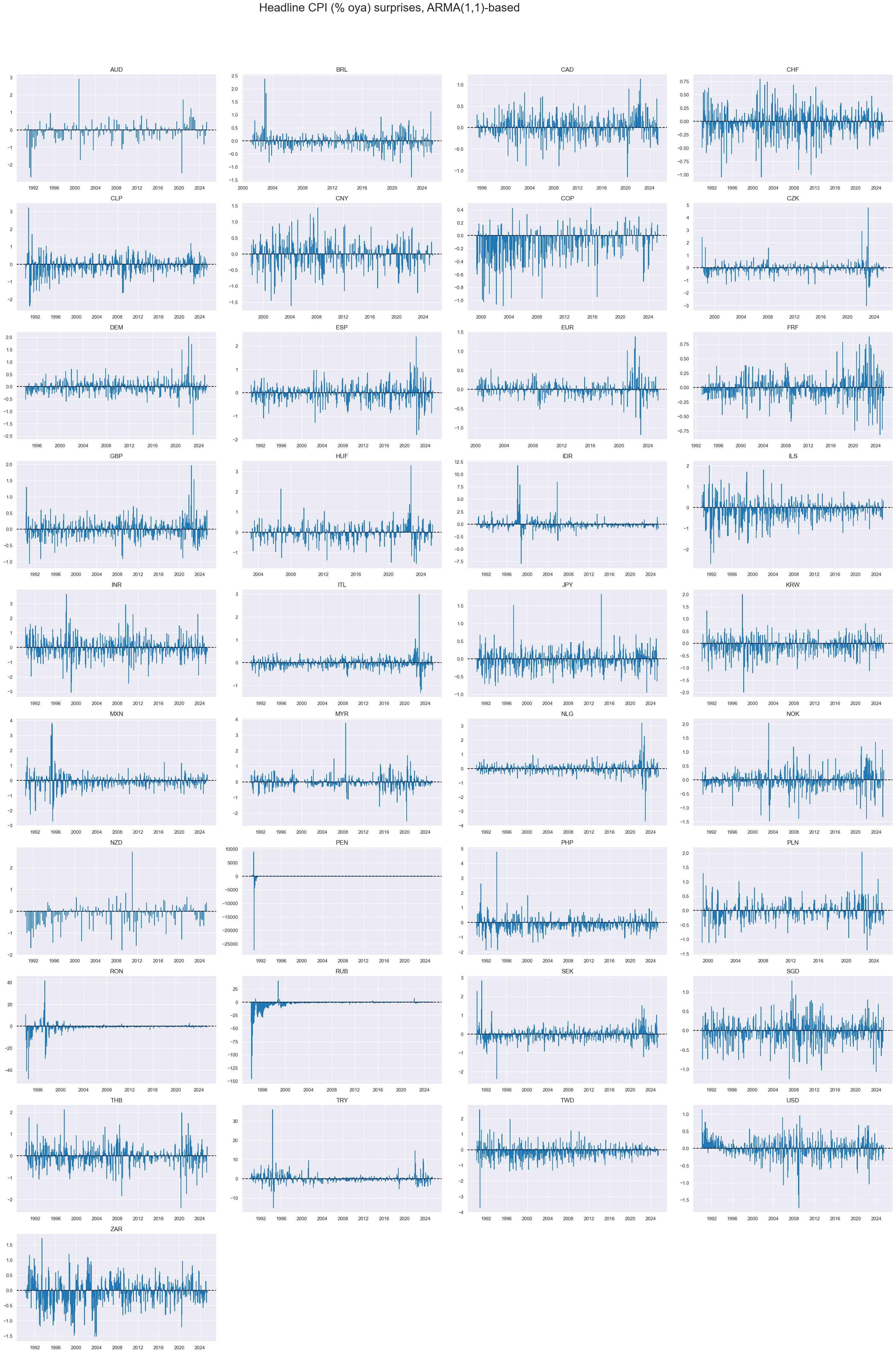
Headline and core CPI inflation surprises are short-term indicators with occasional patterns of mini-cycles.

# Timelines of headline CPI surprises (% oya), ARMA(1,1)-based
# Showing cross-country patterns since 1990

xcatx = ["CPIH_SA_P1M1ML12_ARMAS"]

# Use all available cross-sections
cidx = sorted(cids_exp)

msp.view_timelines(
    dfd,
    xcats=xcatx,
    cids=cidx,
    start=start_date,
    title="Headline CPI (% oya) surprises, ARMA(1,1)-based",
    title_adj=1.02,
    title_xadj=0.435,
    title_fontsize=27,
    legend_fontsize=17,
    label_adj=0.075,
    ncol=4,
    same_y=False,
    size=(12, 7),
    aspect=1.7,
    all_xticks=True,
)

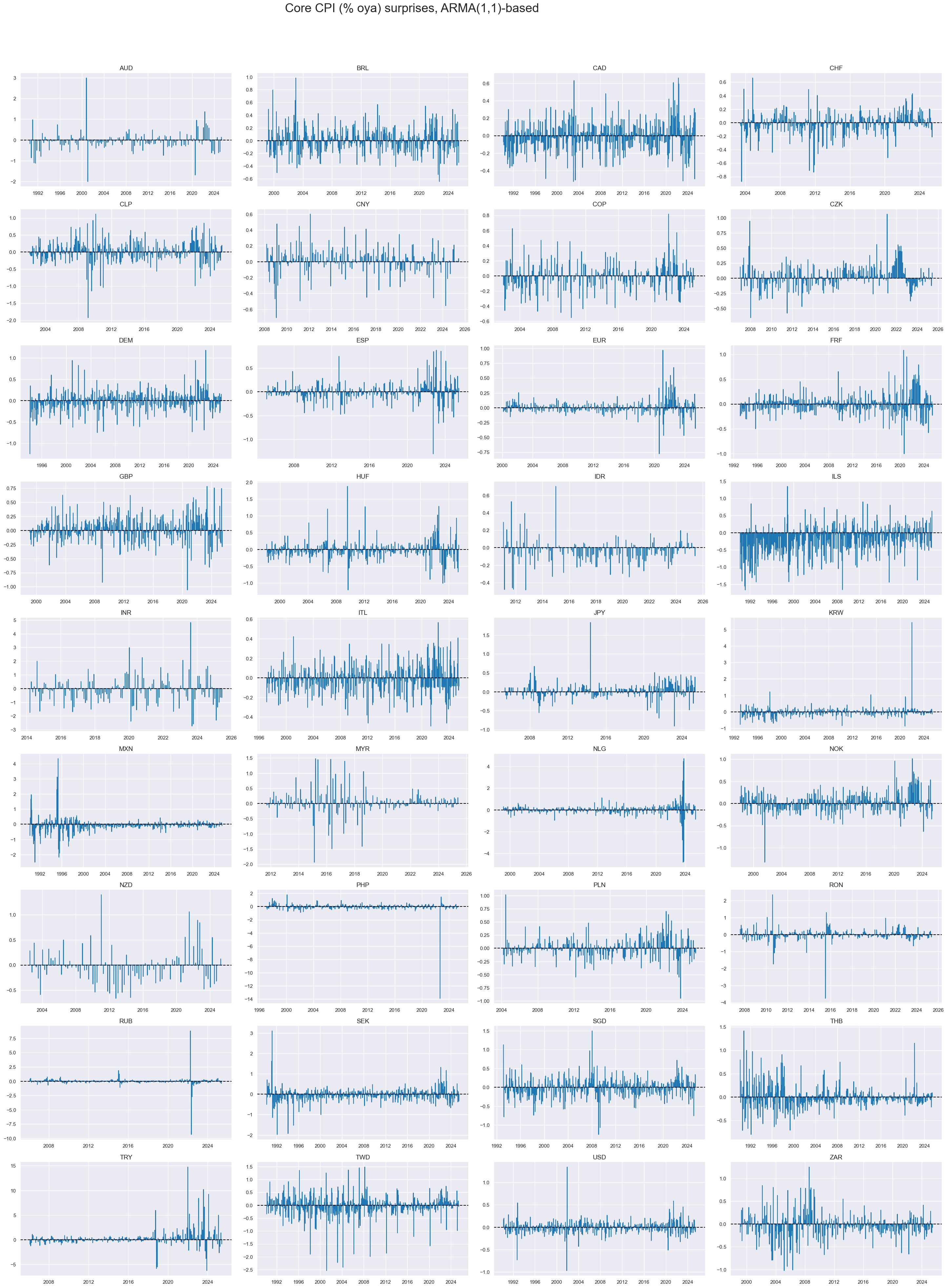
# Timelines of core CPI surprises (% oya), ARMA(1,1)-based
# Excluding PEN due to limited or unreliable coverage

xcatx = ["CPIC_SA_P1M1ML12_ARMAS"]

# Cross-sections to include (exclude PEN)
cidx = sorted(set(cids_exp) - {"PEN"})

msp.view_timelines(
    dfd,
    xcats=xcatx,
    cids=cidx,
    start=start_date,
    title="Core CPI (% oya) surprises, ARMA(1,1)-based",
    title_adj=1.02,
    title_xadj=0.435,
    title_fontsize=27,
    legend_fontsize=17,
    label_adj=0.075,
    ncol=4,
    same_y=False,
    size=(12, 7),
    aspect=1.7,
    all_xticks=True,
)

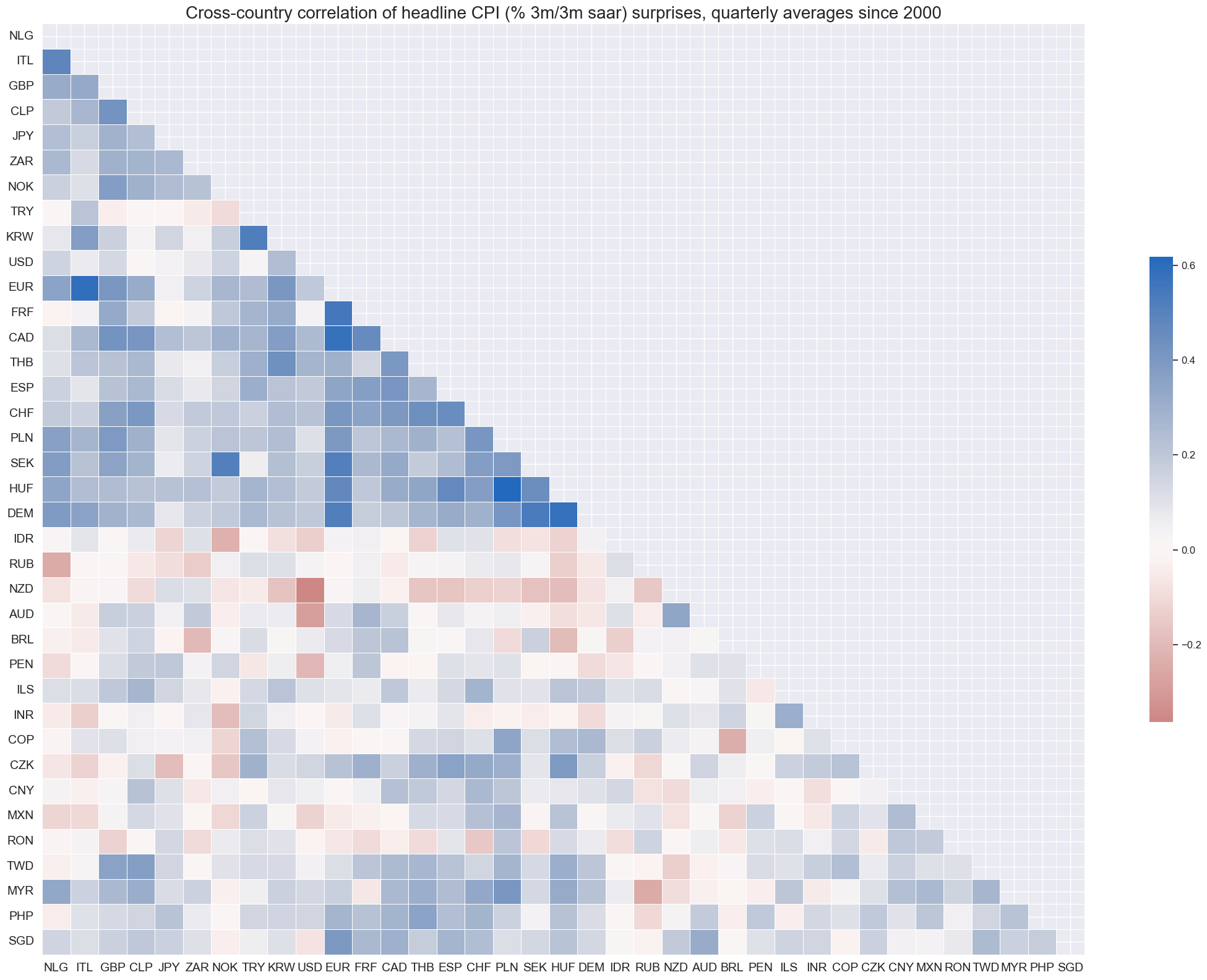
Based on quarterly averages, inflation surprises have been mostly positively correlated internationally, but not uniformly so.

# Cross-country correlation matrix for headline CPI surprises (% 3m/3m annualised), ARMA(1,1)-based
# Based on quarterly averages since 2000

xcatx = "CPIH_SJA_P3M3ML3AR_ARMAS"
cidx = cids_exp

msp.correl_matrix(
    dfd,
    xcats=xcatx,
    cids=cidx,
    freq="q",
    title="Cross-country correlation of headline CPI (% 3m/3m saar) surprises, quarterly averages since 2000",
    cluster=True,
    size=(22, 16),
)

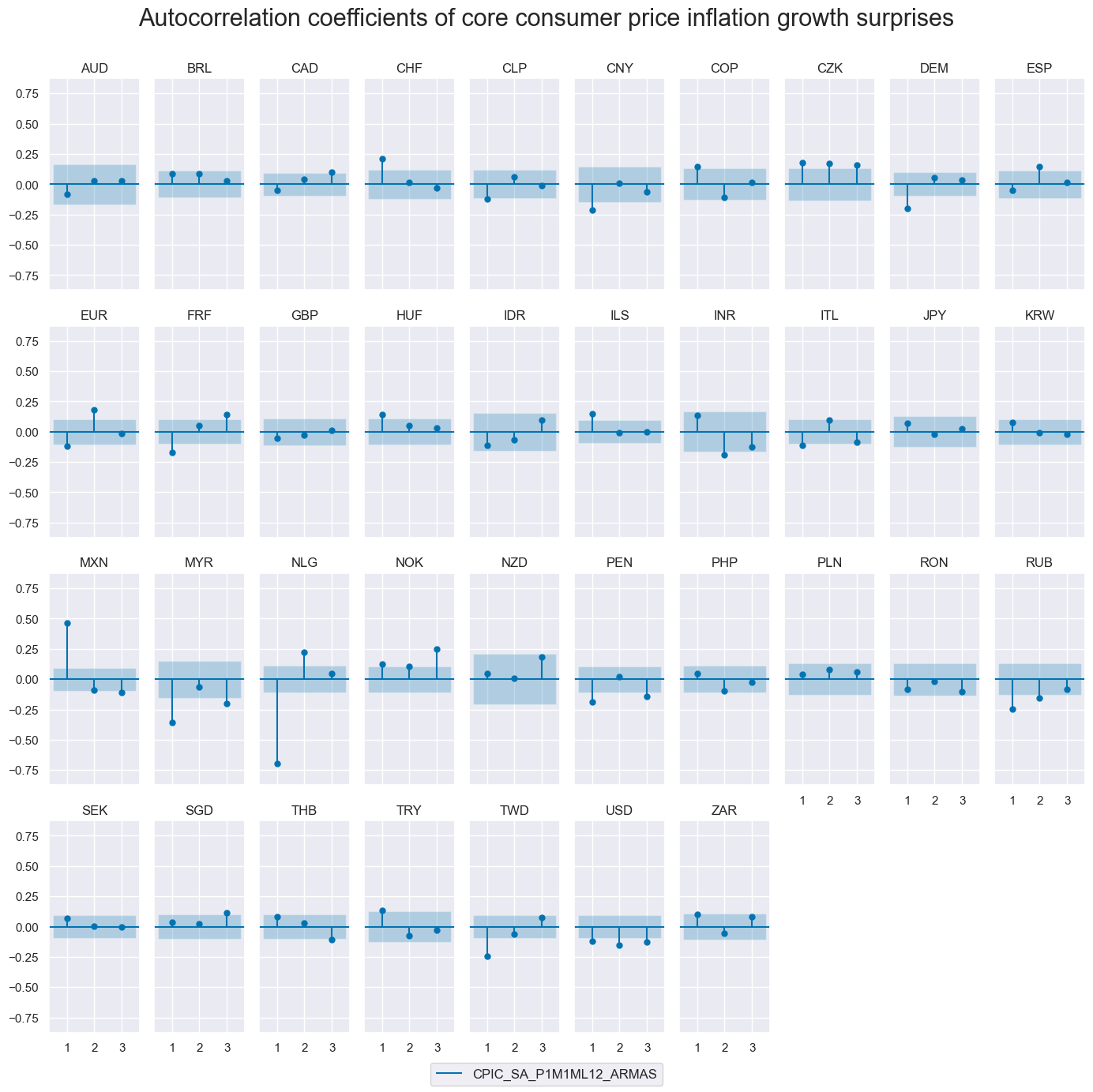
The autocorrelation (ACF) plots assess whether CPI surprise series exhibit temporal dependence. Under the assumption of a well-specified, unbiased one-step-ahead forecast model, real-time surprises should show no systematic autocorrelation.

Most countries conform to this expectation. However, a few — such as Mexico — exhibit residual autocorrelation, likely reflecting episodes of structural inflation shifts or prolonged non-stationarity that challenge the assumptions of the ARMA model.

# Plot PACF of core CPI surprise series (% oya), ARMA(1,1)-based

cidx = sorted(cids_exp)

msv.plot_pacf(
    df=dfd,
    cids=cidx,
    xcat="CPIC_SA_P1M1ML12_ARMAS",
    title="Autocorrelation coefficients of core consumer price inflation growth surprises",
    lags=3,
    remove_zero_predictor=True,
    figsize=(14, 14),
    ncols=10,
)

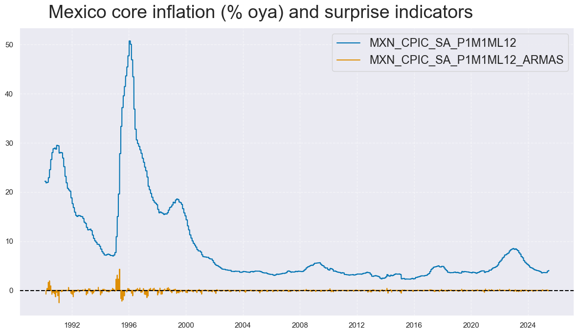
As in the previous analysis, the observed autocorrelation in Mexico’s inflation surprises appears to reflect prolonged periods of non-stationary inflation — particularly during the decline from hyperinflation to price stability. This effect is most visible in the autocorrelation of forecast errors during the 1990s, as illustrated in the chart below.

# Timeline of Mexico core CPI inflation vs. ARMA-based inflation surprises

xcatx = [
    "CPIC_SA_P1M1ML12",          # Core CPI, % oya
    "CPIC_SA_P1M1ML12_ARMAS"     # Surprise in core CPI, % oya
]

cidx = ["MXN"]

msp.view_timelines(
    dfd,
    xcats=xcatx,
    cids=cidx,
    start=start_date,
    title="Mexico core inflation (% oya) and surprise indicators",
    title_adj=1.02,
    title_xadj=0.435,
    title_fontsize=27,
    legend_fontsize=17,
    label_adj=0.075,
    ncol=3,
    same_y=False,
    size=(12, 7),
    aspect=1.7,
    all_xticks=True,
)

Importance

Research links

• The Best Strategies for Inflationary Times (2021)
  Henry Neville, Teun Draaisma, Ben Funnell, Campbell R. Harvey, Otto Van Hemert
  “Unexpected inflation is bad news for traditional assets, such as bonds and equities, with local inflation having the greatest effect. Commodities have positive returns during inflation surges, but there is considerable variation within the commodity complex.”

• A Fundamental Connection: Exchange Rates and Macroeconomic Expectations (2024)
  Vania Stavrakeva, Jenny Tang
  “Exchange rates are strongly influenced by macroeconomic news surprises at business-cycle frequencies, with inflation, activity, and monetary policy surprises all contributing significantly. The effect is particularly strong for lagged surprises — inconsistent with standard models based on uncovered interest parity. The authors document that past inflation surprises explain a large share of medium-term FX variation, especially during recessions or high uncertainty periods, suggesting that macro news, including inflation shocks, is a key driver of currency movements .”

Empirical clues

# Construct an equal-weighted global commodity basket from selected base metals

cids_co = ["ALM", "CPR", "LED", "NIC", "TIN", "ZNC"]  # Aluminium, Copper, Lead, Nickel, Tin, Zinc
cts = [cid + "_" for cid in cids_co]  # Contract identifiers with standard JPMaQS suffix

# Create the basket using 10-day vol-targeted returns
bask_co = msp.Basket(dfd, contracts=cts, ret="COXR_VT10")
bask_co.make_basket(weight_meth="equal", basket_name="GLB")

# Retrieve basket returns and merge into the main dataframe
dfa = bask_co.return_basket()
dfd = msm.update_df(dfd, dfa)

# Construct normalised inflation surprise indicators from consistent CPI trend metrics

xcatx = [
    "CPIC_SA_P1M1ML12_ARMAS",       # Core CPI, monthly trend surprise
    "CPIC_SJA_P3M3ML3AR_ARMAS",     # Core CPI, 3-month adjusted trend surprise
    "CPIC_SJA_P6M6ML6AR_ARMAS",     # Core CPI, 6-month adjusted trend surprise
    "CPIH_SA_P1M1ML12_ARMAS",       # Headline CPI, monthly trend surprise
    "CPIXFE_SA_P1M1ML12_ARMAS",     # Ex-food-and-energy CPI, monthly trend surprise
    "CPIH_SJA_P3M3ML3AR_ARMAS",     # Headline CPI, 3-month adjusted trend surprise
    "CPIH_SJA_P6M6ML6AR_ARMAS",     # Headline CPI, 6-month adjusted trend surprise
    "CPIXFE_SJA_P6M6ML6AR_ARMAS",   # Ex-food-energy CPI, 6-month adjusted trend surprise
    "CPIXFE_SJA_P3M3ML3AR_ARMAS"    # Ex-food-energy CPI, 3-month adjusted trend surprise
]

# Filter cross-sections (excluding Peru)
cidx = list(set(cids_exp) - set(["PEN"]))

# Reduce dataframe to relevant categories and countries
df_red = msm.reduce_df(dfd, xcats=xcatx, cids=cidx)

# Transform to z-scored information state change indicators (standardised surprise signal)
isc_obj = msm.InformationStateChanges.from_qdf(df=df_red, score_by="level")
dfa = isc_obj.to_qdf(value_column="zscore", postfix="N")

# Cap extreme values to +/- 3 standard deviations
dfa["value"] = dfa["value"].clip(lower=-3, upper=3)

# Update main dataframe with the new signals
dfd = msm.update_df(dfd, dfa[["real_date", "cid", "xcat", "value"]])

# Create globally weighted composite indicators for consistent CPI trend surprises

xcatx = [
    "CPIC_SA_P1M1ML12_ARMASN",      # Core CPI, 1-month trend, normalised surprise
    "CPIC_SJA_P3M3ML3AR_ARMASN",    # Core CPI, 3-month trend adjusted, normalised
    "CPIC_SJA_P6M6ML6AR_ARMASN",    # Core CPI, 6-month trend adjusted, normalised
    "CPIH_SA_P1M1ML12_ARMASN",      # Headline CPI, 1-month trend, normalised
    "CPIH_SJA_P3M3ML3AR_ARMASN",    # Headline CPI, 3-month trend adjusted, normalised
    "CPIH_SJA_P6M6ML6AR_ARMASN",    # Headline CPI, 6-month trend adjusted, normalised
    "CPIXFE_SA_P1M1ML12_ARMASN",    # Ex-food-energy CPI, 1-month trend, normalised
    "CPIXFE_SJA_P6M6ML6AR_ARMASN",  # Ex-food-energy CPI, 6-month trend adjusted, normalised
    "CPIXFE_SJA_P3M3ML3AR_ARMASN",  # Ex-food-energy CPI, 3-month trend adjusted, normalised
]

# Exclude Peru and construct global composite for each surprise indicator
cidx = list(set(cids_exp) - set(["PEN"]))

for xc in xcatx:
    dfa = msp.linear_composite(
        df=dfd,
        xcats=xc,
        cids=cidx,
        weights="IVAWGT_SA_1YMA",      # Industry value added weights (1-year moving average)
        new_cid="GLB",                 # Assign composite to synthetic global entity
        complete_cids=False,
    )
    dfd = msm.update_df(dfd, dfa)

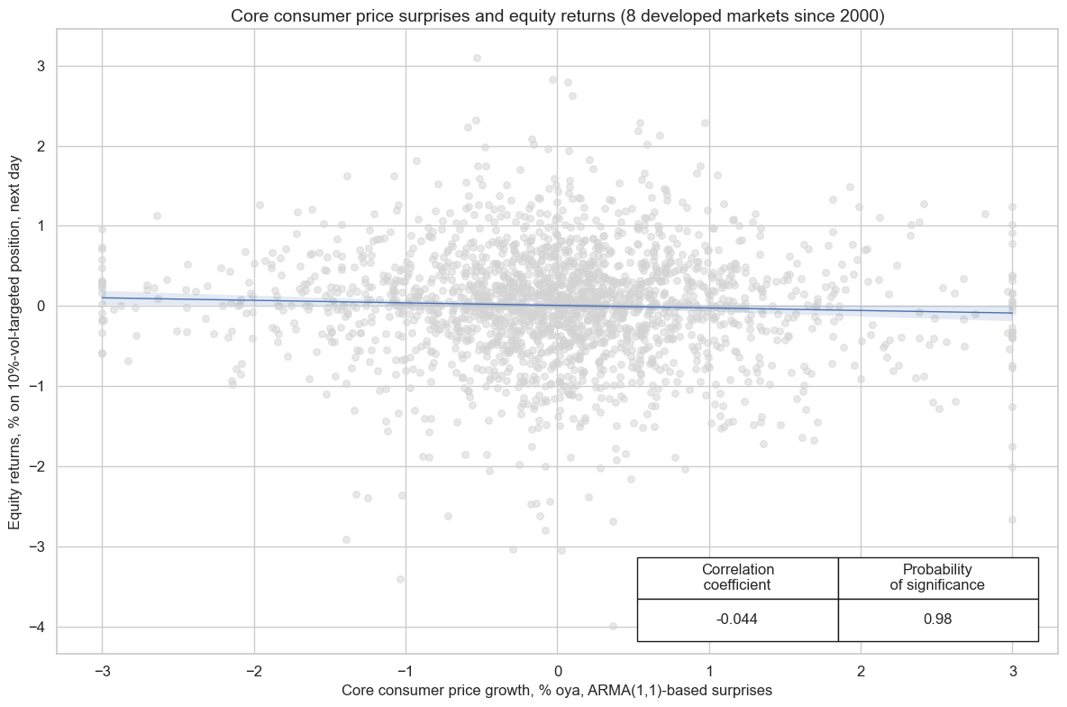
Surprises to core CPI inflation in developed markets can lead to re-assessments of monetary policy. Indeed, daily normalized surprises to core inflation in 8 developed markets with liquid equity index futures have been significant negative predictors of subsequent daily equity returns.

# Assess the predictive relationship between core inflation surprises and next-day equity returns

cr = msp.CategoryRelations(
    dfd,
    xcats=["CPIC_SA_P1M1ML12_ARMASN", "EQXR_VT10"],  # Core CPI surprise and next-day equity returns
    cids=cids_dmca,                                 # Developed market countries
    freq="d",                                       
    lag=1,                                          # One-day forward relationship
    xcat_aggs=["sum", "sum"],                       
    fwin=1,
    start="2000-01-01",
    years=None,
)

cr.reg_scatter(
    coef_box="lower right",
    title="Core consumer price surprises and equity returns (8 developed markets since 2000)",
    xlab="Core consumer price growth, % oya, ARMA(1,1)-based surprises",
    ylab="Equity returns, % on 10%-vol-targeted position, next day",
    prob_est="map",
    remove_zero_predictor=True,
)

EQXR_VT10 misses: ['NOK', 'NZD'].

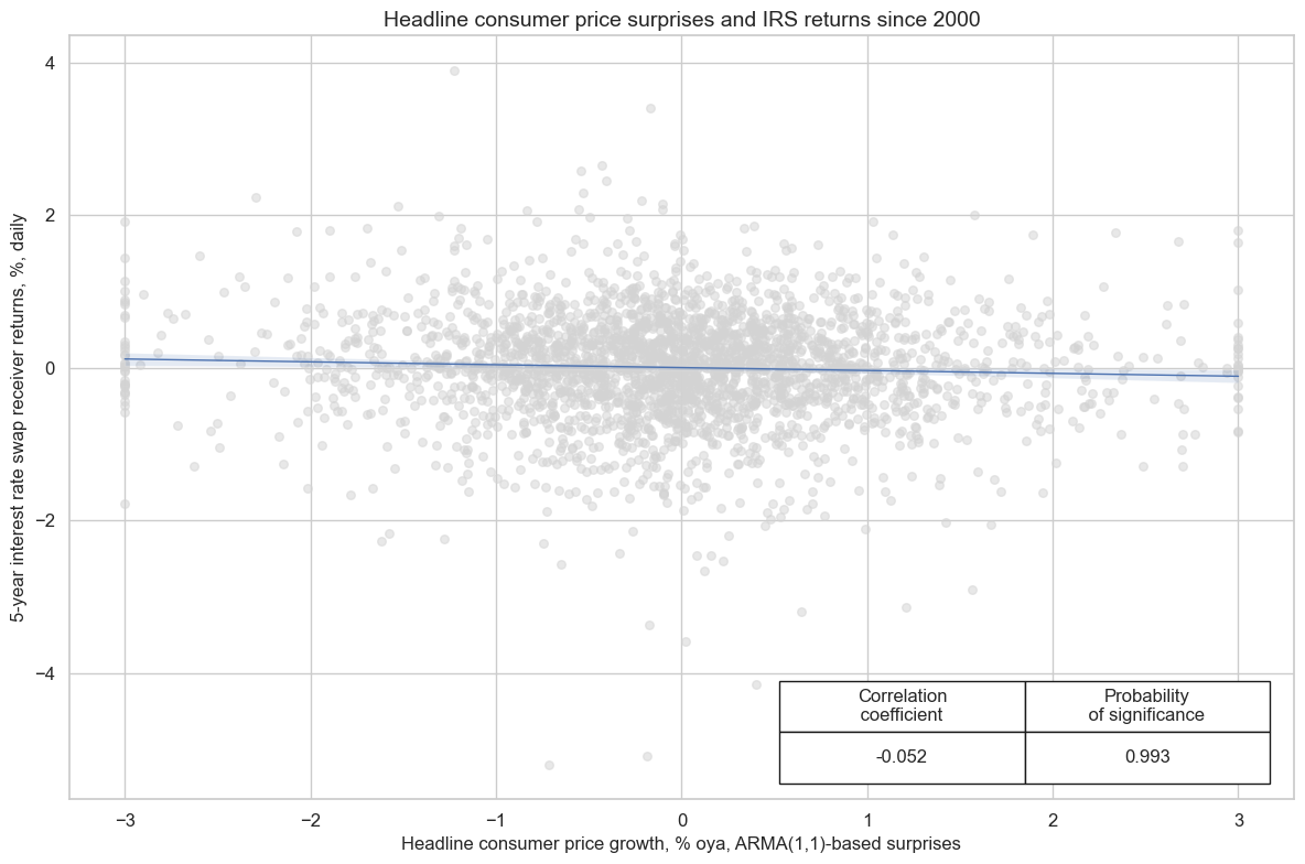
Normalized headline CPI inflation surprises have been signficant negative predictors for next day duration returns, as indicated by 5-year IRS fixed receiver returns.

# Assess the relationship between headline inflation surprises and 5-year IRS returns

cr = msp.CategoryRelations(
    dfd,
    xcats=["CPIH_SA_P1M1ML12_ARMASN", "DU05YXR_VT10"],  # Headline CPI surprise and 5Y IRS receiver return
    cids=cids_dmca,                                     # Developed market countries
    freq="d",                                           
    lag=1,                                              
    xcat_aggs=["sum", "sum"],                          
    fwin=1,
    start="2000-01-01",
    years=None,
)

cr.reg_scatter(
    title="Headline consumer price surprises and IRS returns since 2000",
    labels=False,
    coef_box="lower right",
    xlab="Headline consumer price growth, % oya, ARMA(1,1)-based surprises",
    ylab="5-year interest rate swap receiver returns, %, daily",
    remove_zero_predictor=True,
)

Appendices

Appendix 1: Currency symbols

Cross-sections refer to currencies, currency areas, or economic regions. Codes are grouped below by macro region:

• Developed Markets (DM):
  AUD (Australian dollar), CAD (Canadian dollar), CHF (Swiss franc), EUR (Euro), GBP (British pound),
  JPY (Japanese yen), NOK (Norwegian krone), NZD (New Zealand dollar), SEK (Swedish krona), USD (U.S. dollar).
  Legacy: DEM (German mark), FRF (French franc), ITL (Italian lira), ESP (Spanish peseta), NLG (Dutch guilder)

• EMEA:
  CZK (Czech koruna), HUF (Hungarian forint), PLN (Polish zloty), RON (Romanian leu),
  RUB (Russian ruble), TRY (Turkish lira), ZAR (South African rand)

• APAC:
  CNY (Chinese yuan), HKD (Hong Kong dollar), IDR (Indonesian rupiah), KRW (South Korean won),
  MYR (Malaysian ringgit), PHP (Philippine peso), SGD (Singapore dollar), THB (Thai baht), TWD (Taiwan dollar)

• LATAM:
  BRL (Brazilian real), CLP (Chilean peso), COP (Colombian peso), MXN (Mexican peso), PEN (Peruvian sol)

Appendix 2: Quantamental economic surprises

Quantamental economic surprises are defined as deviations of point-in-time quantamental indicators from expected values. Expectations represent the estimated predictions of an informed market participant. Two types of events contribute to economic surprise indicators:

• First print events
  A first print event is the difference between a quantamental indicator on a release date and its expected value. A release date is the day when any underlying economic time series incorporates a new observation period. Expected values are model-based estimates derived from information available before the release. All surprises are relative to the specific statistical learning or econometric model applied.

• Pure revision events
  A pure revision event is the change in a quantamental indicator on a non-release date, resulting from backward revisions of previously released data. By default, such revisions are assumed to be surprises — the last reported value is treated as the best predictor of the revised value. Revisions published on a release date are included in the first print event.

An economic surprise indicator records the value of these two types of events on the dates they are observed, and zero on all other dates. Prediction models are based on the latest vintage of underlying data and typically forecast increments — such as differences or log differences of volume, value, or price indices.

Notably, this approach means the model first predicts the next period’s increment, then reconstructs the expected index level by adding this increment to the existing series. This reconstructed index automatically captures base effects when calculating growth rates — predictable changes that occur when an unusually sharp move from the base period (such as a year ago) drops out of the calculation. This approach differs from directly forecasting transformed indicators like year-over-year growth rates, which would miss these predictable base effects entirely.

Appendix 3: Advanced-release and first-print surprises

Inflation indicators that incorporate early-released price predictors add a third event to the standard first-print / pure-revision framework in Appendix 2 : the advanced-release surprise , which the surprise of the main indicator that is implied by the release of the early predictor, such as Tokyo CPI for Japan or core CPI for the U.S. (as predictor for core HICP).

Information timeline

In the absence of revisions, there are two events per period :

Event	Timing	Data available	Surprise	Next period expectations
1. Advanced release	Early	Past CPI + predictor	Advanced-release	ARMAX
2. First print	Later	CPI realization	First-print	ARMA

The first print also updates the ARMA model for next period’s baseline expectations.

Surprise definitions

Let \(f(\cdot)\) denote the CPI transformation used in the indicators defined above.

1. Advanced release surprise is the difference between a CPI inflation prediction based on the early-released predictor and the one without it:
   \( u_t^{\text{adv}} \;=\; f\!\bigl(\widehat{PI}_t^{\text{ARMAX}}\bigr) -f\!\bigl(\widehat{PI}_t^{\text{ARMA}}\bigr). \tag{A3.1} \)

2. First-print surprise is the difference between the actual CPI inflation rate and the one predicted based on the early released predictor:
   \( u_t^{\text{fp}} \;=\; f(PI_t) -f\!\bigl(\widehat{PI}_t^{\text{ARMAX}}\bigr). \tag{A3.2} \)

Forecast models

ARMA (baseline)
\( \Delta\ln PI_t =\beta_0 +\beta_1\,\Delta\ln PI_{t-1} +\beta_2\,\varepsilon_{t-1} +\varepsilon_t, \qquad \widehat{\Delta\ln PI}_t^{\text{ARMA}}. \tag{A3.3} \)

ARMAX (predictor-enhanced)
\( \Delta\ln PI_t =\gamma_0 +\gamma_1\,\Delta\ln \text{predictor}_t +\gamma_2\,\Delta\ln PI_{t-1} +\gamma_3\,\xi_{t-1} +\xi_t, \qquad \widehat{\Delta\ln PI}_t^{\text{ARMAX}}. \tag{A3.4} \)

Convert predicted log first-differences back to levels: \( \widehat{PI}_t^{\text{ARMA}} = PI_{t-1}\,\exp\!\bigl(\widehat{\Delta\ln PI}_t^{\text{ARMA}}\bigr), \quad \widehat{PI}_t^{\text{ARMAX}} = PI_{t-1}\,\exp\!\bigl(\widehat{\Delta\ln PI}_t^{\text{ARMAX}}\bigr). \tag{A3.5} \)

Estimation discipline

All variables are expressed as log first-differences . Coefficients are re-estimated for every historical data vintage, ensuring fully out-of-sample forecasts and, therefore, clean real-time macro-surprise series.