Sovereign CDS returns

This group contains various types of generic returns arising from selling protection though sovereign credit default swaps for various maturities and a range of developed and emerging markets.

Sovereign CDS returns

Ticker : CDS02YXR_NSA / CDS05YXR_NSA / CDS10YXR_NSA

Label : Sovereign CDS returns: 2-year maturity / 5-year maturity / 10-year maturity.

Definition : Daily CDS sovereign returns (of protection seller) calculated from the continuous series of CDS spreads: 2-year maturity / 5-year maturity / 10-year maturity.

Notes :

• Returns are calculated from the point of view of the seller of protection, i.e. the CDS seller.

• Return calculation is based on daily rolling rebalancing, whereby each day we use the return of the (constant maturity) CDS contract.

• Returns have been calculated based on CDS spreads from J.P. Morgan DataQuery. The contracts for calculation have changed over time. In 2014, regulation for CDS transactions changed and the new market standard became that of quoting standard coupons. Parties entering CDS contracts since then choose among the available standard coupons and pay or receive the corresponding upfront payment which would make the market value of the CDS equal to zero.

• CDS spreads for emerging markets are ‘par spreads’, as per market convention. The pricing of a par-spread involves using as a coupon whatever the traded spread is at the time of entering the trade.

• CDS spreads for DMs are fixed coupon spreads with coupons of 25bps.

• The calculations are summarized below in Appendix 1 .

Vol-targeted CDS returns

Ticker : CDS02YXR_VT10 / CDS05YXR_VT10 / CDS10YXR_VT10

Label : CDS excess returns for 10% vol target: 2-year maturity / 5-year maturity / 10-year maturity.

Definition : Daily excess returns scaled to 10% (annualized) volatility target: 2-year maturity / 5-year maturity / 10-year maturity.

Notes :

• Positions are scaled to a 10% vol target based on historic standard deviations for an exponential moving average of daily returns with an 11-day half-life of the lookback window. Positions are rebalanced at the end of each month and maximum leverage (notional to risk capital) is constrained to 25.

CDS hedged returns

Ticker : CDS02YXRHvGDRB_NSA / CDS05YXRHvGDRB_NSA / CDS10YXRHvGDRB_NSA

Label : CDS excess returns, hedged against market direction risk: 2-year maturity / 5-year maturity / 10-year maturity.

Definition : Return on a short CDS position that has been hedged against directional risk through a position in a global directional risk basket, %: 2-year maturity / 5-year maturity / 10-year maturity.

Notes :

• The global directional risk basket contains equal volatility-weights in equity index futures, CDS indices and FX forwards. See here for more information on directional risk basket returns ( DRBXR_NSA ).

• Hedge ratios are calculated based on historical “beta”, i.e. weighted least-squares regression coefficients of past returns with respect to global directional risk basket returns. The estimate uses two regressions. One is based on monthly returns with an exponentially-weighted lookback of 24 months half-life. The other is based on daily returns with an exponentially-weighted lookback of 63 trading days. The usage of the two lookbacks seeks to strike a balance between timeliness of information and structural relations.

Imports

Only the standard Python data science packages and the specialized macrosynergy package are needed.

import os
import numpy as np
import pandas as pd
from pandas import Timestamp
import matplotlib.pyplot as plt
import seaborn as sns

import warnings
from datetime import timedelta, date

import macrosynergy.management as msm
import macrosynergy.panel as msp
import macrosynergy.signal as mss
import macrosynergy.pnl as msn
from macrosynergy.download import JPMaQSDownload

import requests
from timeit import default_timer as timer

warnings.simplefilter("ignore")

The JPMaQS indicators we consider are downloaded using the J.P. Morgan Dataquery API interface within the macrosynergy package. This is done by specifying ticker strings , formed by appending an indicator category code <category> to a currency area code <cross_section> . These constitute the main part of a full quantamental indicator ticker, taking the form DB(JPMAQS,<cross_section>_<category>,<info>) , where <info> denotes the time series of information for the given cross-section and category.

The following types of information are available:

• value giving the latest available values for the indicator

• eop_lag referring to days elapsed since the end of the observation period

• mop_lag referring to the number of days elapsed since the mean observation period

• grade denoting a grade of the observation, giving a metric of real time information quality.

After instantiating the JPMaQSDownload class within the macrosynergy.download module, one can use the download(tickers, start_date, metrics) method to obtain the data. Here tickers is an array of ticker strings, start_date is the first release date to be considered and metrics denotes the types of information requested.

# Cross-sections of interest

cids_dmca = ["AUD", "CHF", "GBP", "NOK", "NZD", "SEK", "USD"]
cids_dmeu = [
    "FRF",
    "DEM",
    "ITL",
    "ESP",
]  # DM euro area sovereigns
cids_latm = [
    "BRL",
    "CLP",
    "COP",
    "MXN",
    "PEN",
]  # Latam sovereigns
cids_emea = [
    "CZK",
    "HUF",
    "ILS",
    "PLN",
    "RON",
    "ZAR",
    "TRY",
]  # EMEA sovereigns
cids_emas = [
    "CNY",
    "IDR",
    "KRW",
    "MYR",
    "PHP",
    "THB",
]  # EM Asia sovereigns

cids_dm = cids_dmca + cids_dmeu
cids_em = cids_emea + cids_latm + cids_emas

cids = cids_dm + cids_em

xrets = ["CDS02YXR_NSA", "CDS05YXR_NSA", "CDS10YXR_NSA"]
xvolrets = ["CDS02YXR_VT10", "CDS05YXR_VT10", "CDS10YXR_VT10"]
hedge_rets = ["CDS02YXRHvGDRB_NSA", "CDS05YXRHvGDRB_NSA", "CDS10YXRHvGDRB_NSA"]

main = xrets + xvolrets + hedge_rets
xtra = ["GB05YXR_NSA", "GB10YXR_NSA"]
xcats = main + xtra

# Resultant tickers

tickers = [cid + "_" + xcat for cid in cids for xcat in xcats]
print(f"Maximum number of tickers is {len(tickers)}")

Maximum number of tickers is 319

# Download series from J.P. Morgan DataQuery by tickers

start_date = "1996-01-01"
tickers = [cid + "_" + xcat for cid in cids for xcat in xcats]
print(f"Maximum number of tickers is {len(tickers)}")

# Retrieve credentials

client_id: str = os.getenv("DQ_CLIENT_ID")
client_secret: str = os.getenv("DQ_CLIENT_SECRET")

# Download from DataQuery

with JPMaQSDownload(client_id=client_id, client_secret=client_secret) as downloader:
    start = timer()
    df = downloader.download(
        tickers=tickers,
        start_date=start_date,
        metrics=["value", "eop_lag", "mop_lag", "grading"],
        suppress_warning=True,
        show_progress=True,
    )
    end = timer()

dfd = df

print("Download time from DQ: " + str(timedelta(seconds=end - start)))

Maximum number of tickers is 319
Downloading data from JPMaQS.
Timestamp UTC:  2024-02-23 12:34:32

Connection successful!

Requesting data: 100%|██████████| 64/64 [00:15<00:00,  4.12it/s]
Downloading data: 100%|██████████| 64/64 [00:17<00:00,  3.74it/s]

Some expressions are missing from the downloaded data. Check logger output for complete list.
180 out of 1276 expressions are missing. To download the catalogue of all available expressions and filter the unavailable expressions, set `get_catalogue=True` in the call to `JPMaQSDownload.download()`.
Some dates are missing from the downloaded data. 
3 out of 7347 dates are missing.
Download time from DQ: 0:00:36.831920

Availability

cids_exp = sorted(list(cids))  # cids expected in category panels
msm.missing_in_df(dfd, xcats=main, cids=cids_exp)

Missing xcats across df:  []

Missing cids for CDS02YXRHvGDRB_NSA:  ['PHP']
Missing cids for CDS02YXR_NSA:  []
Missing cids for CDS02YXR_VT10:  []
Missing cids for CDS05YXRHvGDRB_NSA:  ['PHP']
Missing cids for CDS05YXR_NSA:  []
Missing cids for CDS05YXR_VT10:  []
Missing cids for CDS10YXRHvGDRB_NSA:  ['PHP']
Missing cids for CDS10YXR_NSA:  []
Missing cids for CDS10YXR_VT10:  []

Starting dates for sovereign CDS returns are mixed. For most cross-sections, data is available only from the mid-2000s onwards. The only countries for which data are available from the 1990s are Brazil, Colombia, Mexico and Poland.

For the explanation of currency symbols, which are related to currency areas or countries for which categories are available, please view Appendix 2 .

xcatx = main
cidx = cids_exp

dfx = msm.reduce_df(dfd, xcats=xcatx, cids=cidx)
dfs = msm.check_startyears(
    dfx,
)
msm.visual_paneldates(dfs, size=(18, 6))

print("Last updated:", date.today())

Last updated: 2024-02-23

xcatx = main
cidx = cids_exp

plot = msm.check_availability(
    dfd, xcats=xcatx, cids=cidx, start_size=(18, 3), start_years=False
)

xcatx = main
cidx = cids_exp

plot = msp.heatmap_grades(
    dfd,
    xcats=xcatx,
    cids=cidx,
    size=(18, 6),
    title=f"Average vintage grades from {start_date} onwards",
)

xcatx = ["CDS02YXR_NSA", "CDS05YXR_NSA"]

msp.view_ranges(
    dfd,
    xcats=xcatx,
    cids=cids,
    val="eop_lag",
    title="End of observation period lags (ranges of time elapsed since end of observation period in days)",
    start="2000-01-01",
    kind="box",
    size=(16, 4),
)

History

CDS returns

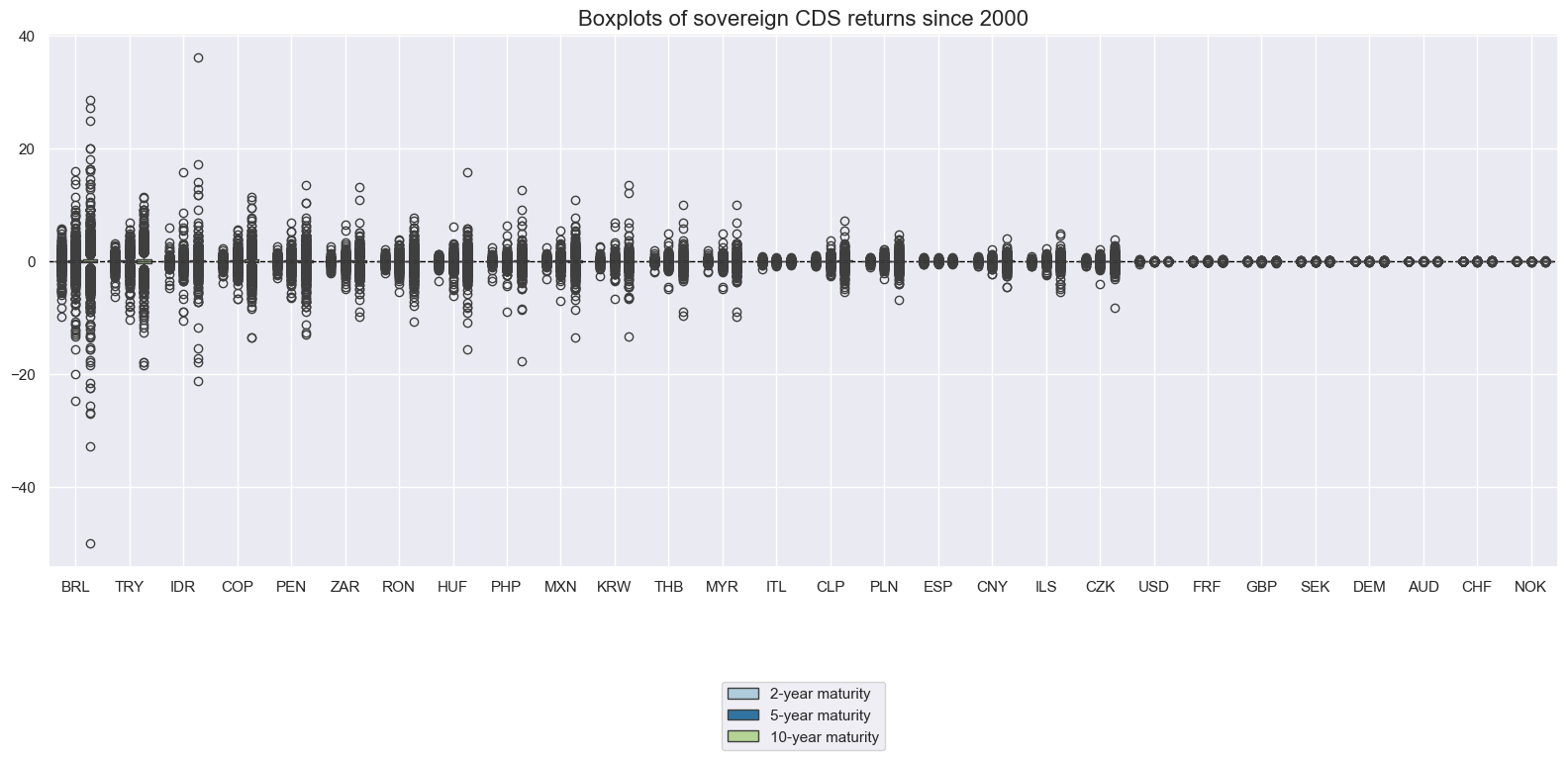
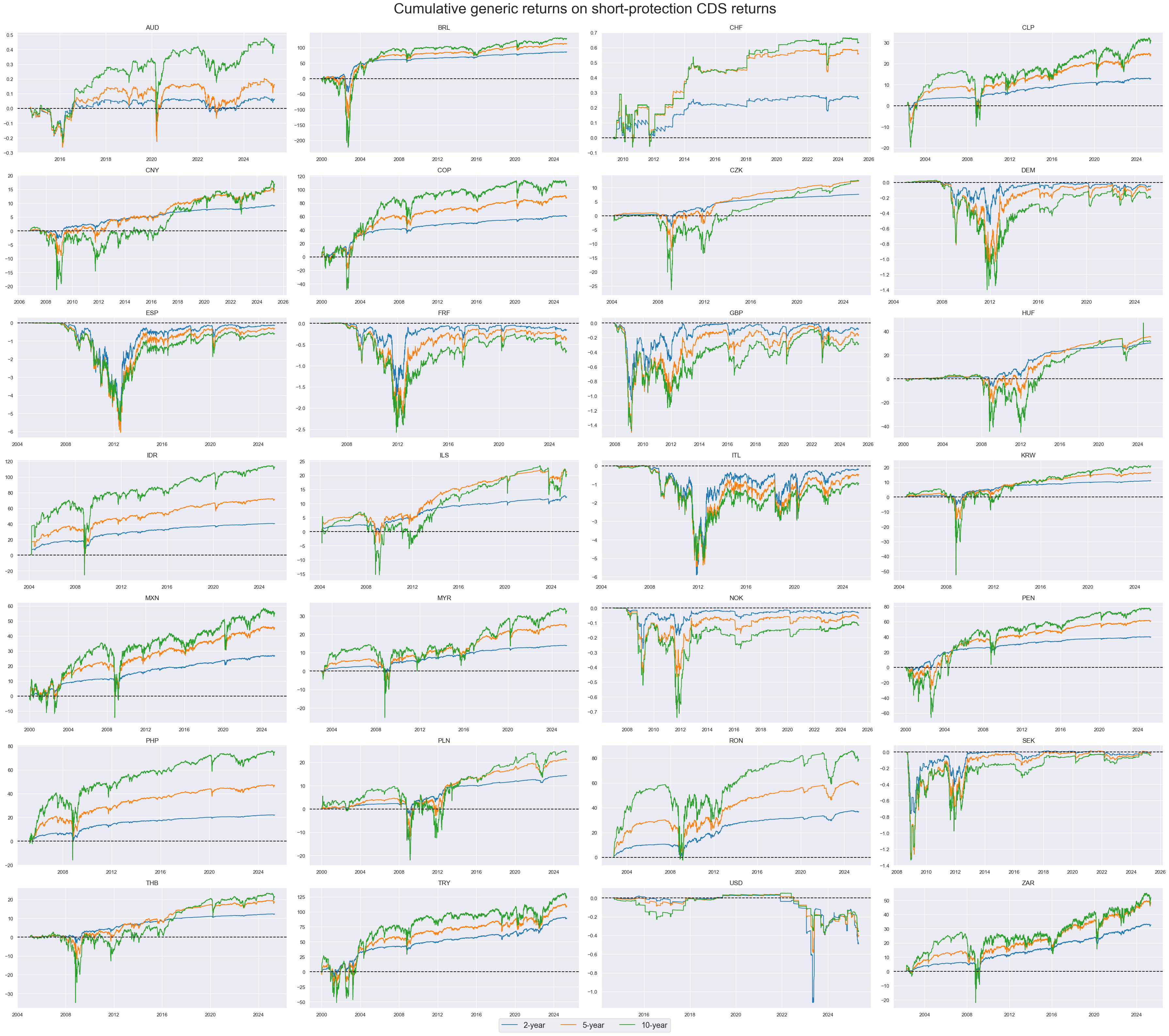
Selling protection through CDS means taking credit risk. This is akin to writing an option and leads to non-linear returns with large outliers. Long-term cumulative generic returns have been negative for many countries since the inception of the CDS market. This partly reflects the prevalence of credit crises in the late 2000s and early 2010s. Naturally variation of returns for high-risk countries has been a lot higher than for countries with low sovereign credit risk.

xcatx = xrets
cidx = cids_exp

msp.view_ranges(
    dfd,
    xcats=xcatx,
    cids=cidx,
    sort_cids_by="std",
    start="2000-01-01",
    kind="box",
    title="Boxplots of sovereign CDS returns since 2000",
    xcat_labels=["2-year maturity", "5-year maturity", "10-year maturity"],
    size=(16, 8),
)

xcatx = xrets
cidx = cids_exp

msp.view_timelines(
    dfd,
    xcats=xcatx,
    cids=cidx,
    start="2000-01-01",
    title="Cumulative generic returns on short-protection CDS returns",
    title_fontsize=32,
    legend_fontsize=17,
    xcat_labels=["2-year", "5-year", "10-year"],
    label_adj=0.075,
    cumsum=True,
    ncol=4,
    same_y=False,
    height=3,
    aspect=2,
    all_xticks=True,
)

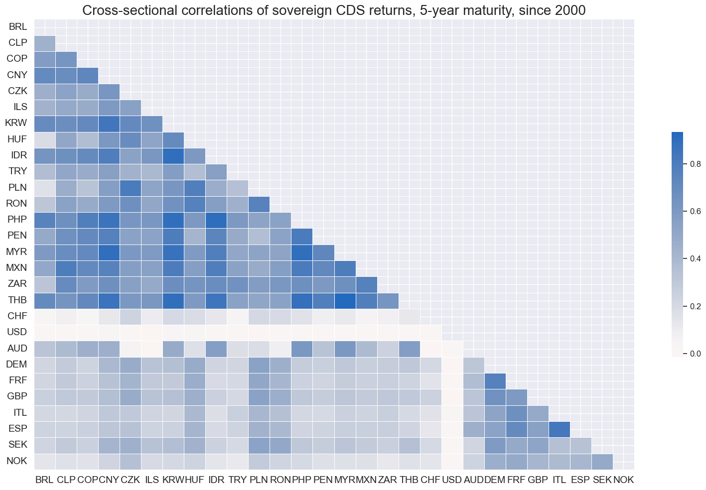
CDS returns have generally been positively correlated, particularly for emerging markets. This is not surprising as the CDS market is a global market and the risk of a credit crisis is a global phenomenon. The correlation between CDS returns for developed markets has been lower, but still positive.

msp.correl_matrix(
    dfd,
    xcats="CDS05YXR_NSA",
    cids=cids,
    size=(16, 10),
    cluster=True,
    start="2000-01-01",
    freq="W",
    title="Cross-sectional correlations of sovereign CDS returns, 5-year maturity, since 2000",
)

Vol-targeted CDS excess returns

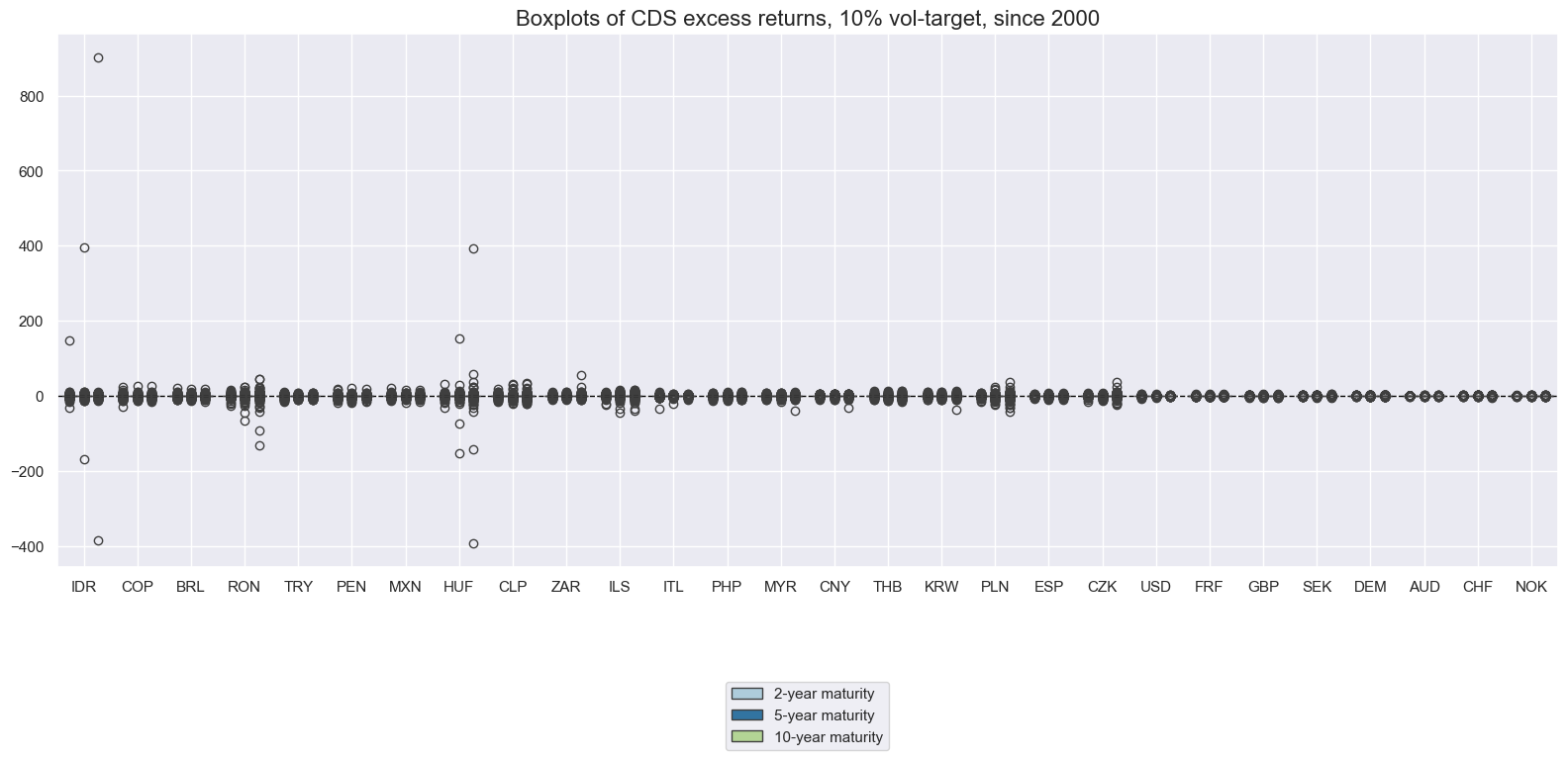
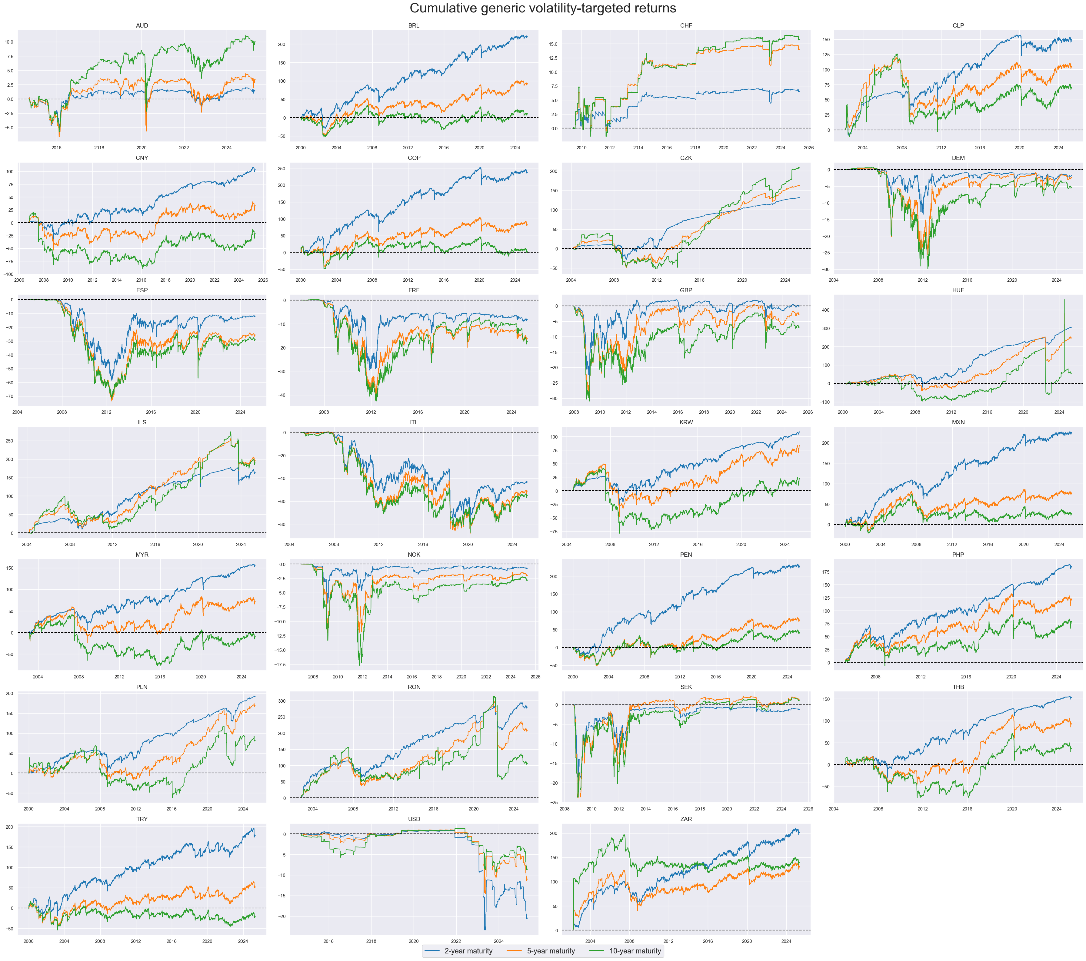
Volatility-targeting makes returns more comparable across tenors and countries. However, the leverage limit of 25 chosen for the system still restricts the volatility with very low risk spreads.

The consistency of negative returns for some EM countries over the past 20 years contracts the notion of premia for investors taking sovereign credit risk exposure through the CDS market.

xcatx = xvolrets
cidx = cids

msp.view_ranges(
    dfd,
    xcats=xcatx,
    cids=cidx,
    sort_cids_by="std",
    start="2000-01-01",
    kind="box",
    title="Boxplots of CDS excess returns, 10% vol-target, since 2000",
    xcat_labels=["2-year maturity", "5-year maturity", "10-year maturity"],
    size=(16, 8),
)

xcatx = xvolrets
cidx = cids

msp.view_timelines(
    dfd,
    xcats=xcatx,
    cids=cidx,
    start="2000-01-01",
    title="Cumulative generic volatility-targeted returns",
    title_fontsize=32,
    legend_fontsize=17,
    xcat_labels=["2-year maturity", "5-year maturity", "10-year maturity"],
    label_adj=0.05,
    cumsum=True,
    ncol=4,
    same_y=True,
    height=3,
    aspect=2,
    all_xticks=True,
)

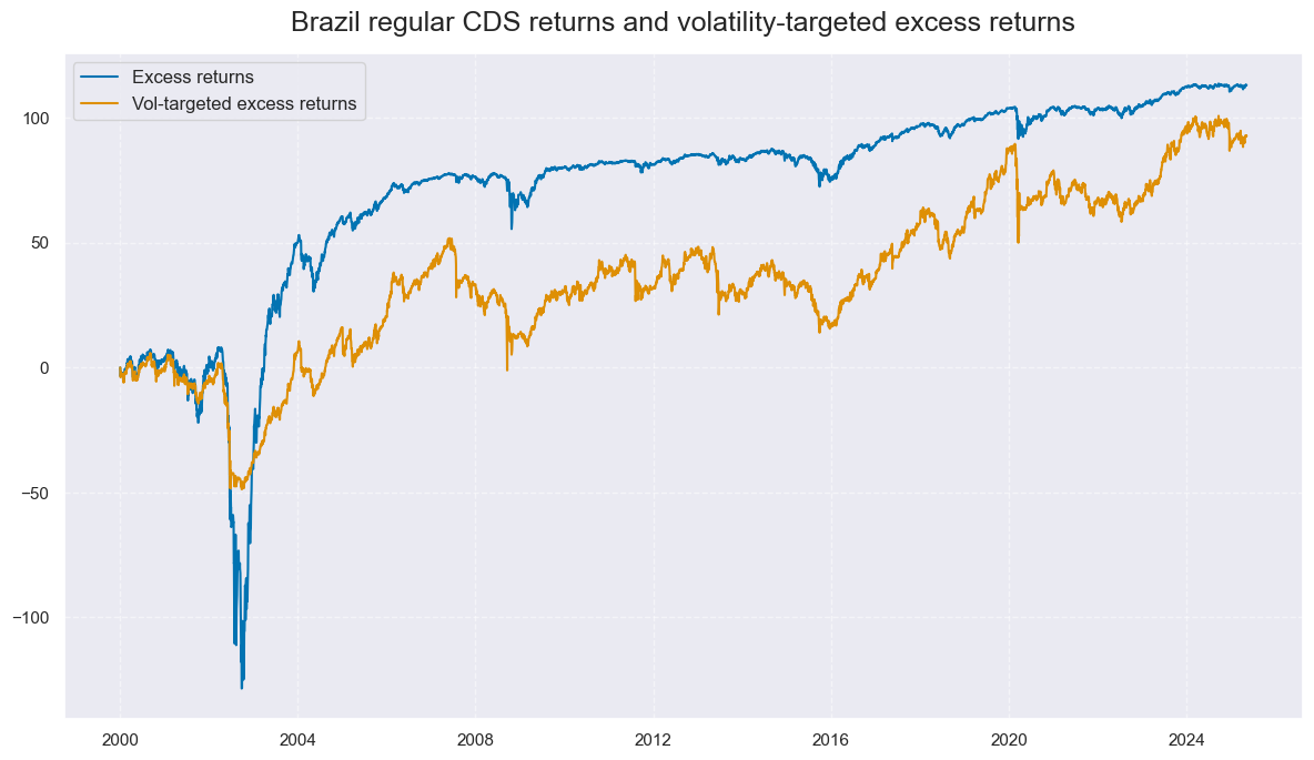
The history of Brazil’s CDS returns provides two interesting lessons:

• The surge in spreads in June 2002 illustrates the non-linear impact of rising default risk. Volatility-adjusted returns, which rely on monthly rebalancing in our data set, have faired little better than outright returns and actually experienced an even greater shock relative to their variation in normal times.

• Vol-targeting led to consistent negative returns. While notional returns often fully recovered after sell-offs, vol-targeted positioning has typicall reduced notional exposure.

xcatx = ["CDS05YXR_NSA", "CDS05YXR_VT10"]
cidx = ["BRL"]

msp.view_timelines(
    dfd,
    xcats=xcatx,
    cids=cidx,
    start="2000-01-01",
    title="Brazil regular CDS returns and volatility-targeted excess returns",
    title_adj=1.02,
    xcat_labels=["Excess returns", "Vol-targeted excess returns"],
    cumsum=True,
    ncol=3,
    same_y=False,
    size=(12, 7),
    all_xticks=True,
)

Hedged CDS returns

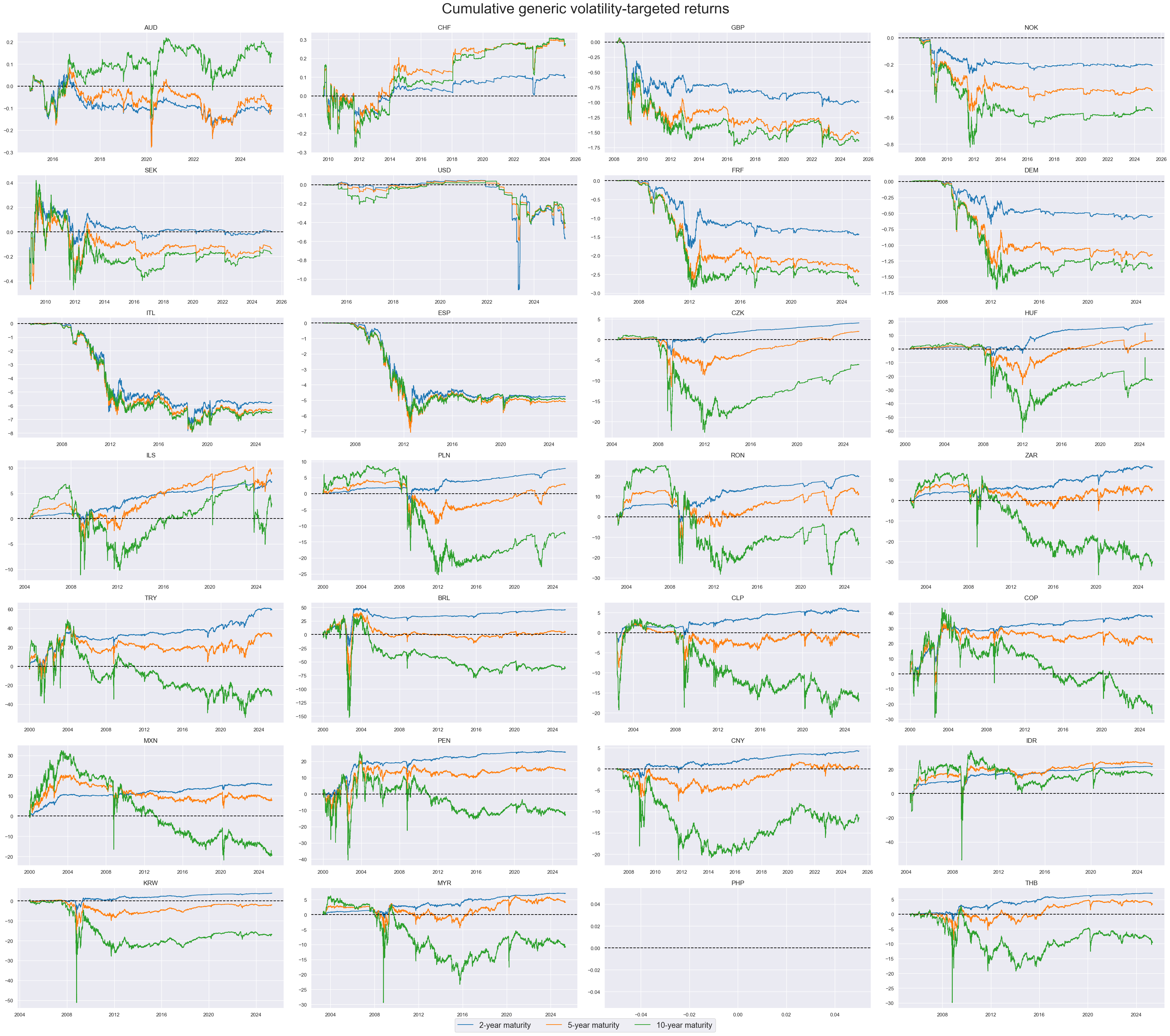
The sensitivity of sovereign CDS to returns in a global risk basket (that contain in equal weight: credit, equity and FX) typically depends on (i) the concurrent vulnerability of sovereign finances, (ii) the prevalence of systemic risk and (iii) the dominance of credit concerns in financial markets.

Hedged CDS protection selling positions would have been mostly loss making.

xcatx = hedge_rets
cidx = cids

msp.view_timelines(
    dfd,
    xcats=xcatx,
    cids=cidx,
    start="2000-01-01",
    title="Cumulative generic volatility-targeted returns",
    title_fontsize=32,
    legend_fontsize=17,
    xcat_labels=["2-year maturity", "5-year maturity", "10-year maturity"],
    label_adj=0.08,
    cumsum=True,
    ncol=4,
    same_y=False,
    height=3,
    aspect=2,
    all_xticks=True,
)

Importance

Relevant research

“Sovereign CDS spreads are highly driven by liquidity (55.6% of default risk and 44.32% of liquidity) and that sovereign bond spreads are less subject to liquidity frictions and therefore could represent a better proxy for sovereign default risk (73% of default risk and 26.86% of liquidity).” Badaoui, Cathcart and El-Jahel

Empirical clues

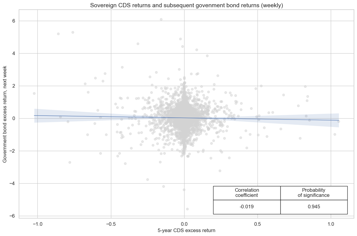
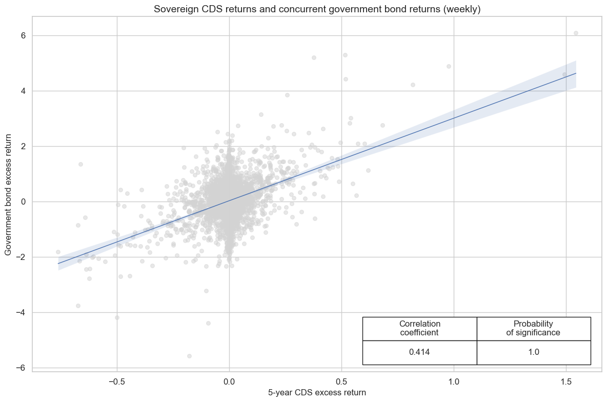
Interestingly, CDS returns have negatively predicted subsequent bond returns in developed markets. Thus, sell-offs in the CDS market have tended to give way to subsequent recoveries in bond markets. This may reflect the difficult liquidity situation in CDS markets which may lead to exaggerated liquidity-driven moves that spill over concurrently into bonds, as well the tendency of policymakers to become more supportive in words and actions in the face of serious credit risks.

xcatx = ["CDS05YXR_NSA", "GB05YXR_NSA"]
cidx = ["AUD", "DEM", "FRF", "ESP", "ITL", "NZD", "GBP", "USD"]

cr = msp.CategoryRelations(
    dfd,
    xcats=xcatx,
    cids=cidx,
    xcat_aggs=["sum", "sum"],
    freq="W",
    lag=1,
    slip=1,  # one-day slippage to avoid time zone distortions
    start="2000-01-01",
    years=None,
)

cr.reg_scatter(
    title="Sovereign CDS returns and subsequent govenment bond returns (weekly)",
    labels=False,
    coef_box="lower right",
    ylab="Government bond excess return, next week",
    xlab="5-year CDS excess return",
    prob_est="map",
)

xcatx = ["CDS05YXR_NSA", "GB05YXR_NSA"]
cidx = ["AUD", "DEM", "FRF", "ESP", "ITL", "NZD", "GBP", "USD"]

cr = msp.CategoryRelations(
    dfd,
    xcats=xcatx,
    xcat_aggs=["sum", "sum"],
    cids=cidx,
    freq="W",
    lag=0,
    start="2000-01-01",
    years=None,
)

cr.reg_scatter(
    title="Sovereign CDS returns and concurrent government bond returns (weekly)",
    labels=False,
    coef_box="lower right",
    ylab="Government bond excess return",
    xlab="5-year CDS excess return",
    prob_est="map",
)

Appendices

Appendix 1: Calculation of total and excess generic bond returns

Excess returns are calculated by following the method of Augustin et al . It is a simplification of the true cash-flow return of a CDS, which is 99% correlated with actual CDS returns. It involves computing the difference between the spread and the coupon, taking its net present value according to the short term interest rate and adjusting it by a factor that takes into account the short term interest rate and the recovery rate.

The price of a CDS is:

(15) \[\begin{equation} {P}_{t} = {\frac{(S_{t} - c)} {(r_{t} + {\frac{S_{t}}{(1-R)}} )}} (1-e^{-(r_{t} + {\frac{S_{t}}{(1-R)}} )(T-t)}) \end{equation}\]

where:

S is the CDS spread, c is the coupon, r is the annualised short-term funding rate (as approximated by the local interbank or a collateralised funding rate), T is the tenor of your lookup period and t is the current time.

The return, adjusting for the unfunded nature of the CDS position, will therefore be the difference between the price of today and tomorrow (divided by the notional of the contract, which is 1 ):

(16) \[\begin{equation} {R}_{t, t+1} = {P}_{t+1} - {P}_{t} \end{equation}\]

We can use this formula only for fixed-coupon CDSs. Credit defaults swaps of EM countries have histories of par-coupons, whereby the coupon was set at the same level as the spread on the initiation date. Hence we use the simple formula for returns equal to the difference between the prices in two respective days. In the case of CDS traded at par, the formula we use is the simple difference between spreads:

(17) \[\begin{equation} {R}_{t, t+1} = {S}_{t+1} - {S}_{t} \end{equation}\]

where S is the spread at close of the day.

Appendix 2: Currency symbols

The word ‘cross-section’ refers to currencies, currency areas or economic areas. In alphabetical order, these are AUD (Australian dollar), BRL (Brazilian real), CAD (Canadian dollar), CHF (Swiss franc), CLP (Chilean peso), CNY (Chinese yuan renminbi), COP (Colombian peso), CZK (Czech Republic koruna), DEM (German mark), ESP (Spanish peseta), EUR (Euro), FRF (French franc), GBP (British pound), HKD (Hong Kong dollar), HUF (Hungarian forint), IDR (Indonesian rupiah), ITL (Italian lira), JPY (Japanese yen), KRW (Korean won), MXN (Mexican peso), MYR (Malaysian ringgit), NLG (Dutch guilder), NOK (Norwegian krone), NZD (New Zealand dollar), PEN (Peruvian sol), PHP (Phillipine peso), PLN (Polish zloty), RON (Romanian leu), RUB (Russian ruble), SEK (Swedish krona), SGD (Singaporean dollar), THB (Thai baht), TRY (Turkish lira), TWD (Taiwanese dollar), USD (U.S. dollar), ZAR (South African rand).