Imports #
Only the standard Python data science packages and the specialized
macrosynergy
package are needed.
import os
import numpy as np
import pandas as pd
import matplotlib.pyplot as plt
import seaborn as sns
import math

import json
import yaml

import macrosynergy.management as msm
import macrosynergy.panel as msp
import macrosynergy.signal as mss
import macrosynergy.pnl as msn
from macrosynergy.download import JPMaQSDownload

from timeit import default_timer as timer
from datetime import timedelta, date, datetime

import warnings

warnings.simplefilter("ignore")
The
JPMaQS
indicators we consider are downloaded using the J.P. Morgan Dataquery API interface within the
macrosynergy
package. This is done by specifying
ticker strings
, formed by appending an indicator category code
<category>
to a currency area code
<cross_section>
. These constitute the main part of a full quantamental indicator ticker, taking the form
DB(JPMAQS,<cross_section>_<category>,<info>)
, where
<info>
denotes the time series of information for the given cross-section and category. The following types of information are available:
-
valuegiving the latest available values for the indicator -
eop_lagreferring to days elapsed since the end of the observation period -
mop_lagreferring to the number of days elapsed since the mean observation period -
gradedenoting a grade of the observation, giving a metric of real time information quality.
After instantiating the
JPMaQSDownload
class within the
macrosynergy.download
module, one can use the
download(tickers,start_date,metrics)
method to easily download the necessary data, where
tickers
is an array of ticker strings,
start_date
is the first collection date to be considered and
metrics
is an array comprising the times series information to be downloaded.
# Cross-sections of interest

cids_dm = ["AUD", "CAD", "CHF", "EUR", "GBP", "JPY", "NOK", "NZD", "SEK", "USD"]
cids_dmec = ["DEM", "ESP", "FRF", "ITL", "NLG"]
cids_latm = ["BRL", "COP", "CLP", "MXN", "PEN"]
cids_emea = ["CZK", "HUF", "ILS", "PLN", "RON", "RUB", "TRY", "ZAR"]
cids_emas = ["CNY", "HKD", "IDR", "INR", "KRW", "MYR", "PHP", "SGD", "THB", "TWD"]
cids_em = cids_latm + cids_emea + cids_emas

cids = sorted(cids_dm + cids_em)
# Quantamental categories of interest

main = [
    "USDGDPWGT_SA_1YMA",
    "USDGDPWGT_SA_3YMA",
    "PPPGDPWGT_NSA_1YMA",
    "PPPGDPWGT_NSA_3YMA",
    "IVAWGT_SA_1YMA",
    "IVAWGT_SA_3YMA",
]
econ = [
    "CABGDPRATIO_NSA_12MMA",
    "INTRGDPv5Y_NSA_P1M1ML12_3MMA",
    "MTBGDPRATIO_SA_3MMAv24MMA",
]  # economic context
mark = ["FXXR_VT10", "FXCRR_VT10", "EQXR_NSA", "DU05YXR_VT10"]  # market data

xcats = main + econ + mark
# Download series from J.P. Morgan DataQuery by tickers

start_date = "1995-01-01"
tickers = [cid + "_" + xcat for cid in cids for xcat in xcats]
print(f"Maximum number of tickers is {len(tickers)}")

# Retrieve credentials

client_id: str = os.getenv("DQ_CLIENT_ID")
client_secret: str = os.getenv("DQ_CLIENT_SECRET")

# Download from DataQuery

with JPMaQSDownload(client_id=client_id, client_secret=client_secret) as downloader:
    start = timer()
    df = downloader.download(
        tickers=tickers,
        start_date=start_date,
        metrics=["value", "eop_lag", "mop_lag", "grading"],
        suppress_warning=True,
        show_progress=True,
    )
    end = timer()

dfd = df

print("Download time from DQ: " + str(timedelta(seconds=end - start)))
Maximum number of tickers is 429
Downloading data from JPMaQS.
Timestamp UTC:  2024-03-27 11:50:08
Connection successful!
Requesting data: 34%|███▎ | 29/86 [00:05<00:11, 4.96it/s]
Requesting data: 100%|██████████| 86/86 [00:18<00:00,  4.55it/s]
Downloading data: 100%|██████████| 86/86 [00:31<00:00,  2.76it/s]
Some expressions are missing from the downloaded data. Check logger output for complete list.
92 out of 1716 expressions are missing. To download the catalogue of all available expressions and filter the unavailable expressions, set `get_catalogue=True` in the call to `JPMaQSDownload.download()`.
Some dates are missing from the downloaded data.
2 out of 7630 dates are missing.
Download time from DQ: 0:00:57.107659
Availability #
cids_exp = sorted(
    list(set(cids) - set(cids_dmec + ["ARS", "HKD", "CZK"]))
)  # cids expected in category panels
msm.missing_in_df(dfd, xcats=main, cids=cids_exp)
Missing xcats across df:  []
Missing cids for IVAWGT_SA_1YMA:      []
Missing cids for IVAWGT_SA_3YMA:      []
Missing cids for PPPGDPWGT_NSA_1YMA:  []
Missing cids for PPPGDPWGT_NSA_3YMA:  []
Missing cids for USDGDPWGT_SA_1YMA:   []
Missing cids for USDGDPWGT_SA_3YMA:   []
dfx = msm.reduce_df(dfd, xcats=main, cids=cids_exp)
dfs = msm.check_startyears(dfx)
msm.visual_paneldates(dfs, size=(18, 6))

Most GDP weights are presently available from the mid-1990s.
plot = msm.check_availability(dfd, xcats=main, cids=cids_exp, start_size=(20, 4))


PPP-adjusted GDP weights have the lowest grades at present, for lack of original vintages from source.
plot = msp.heatmap_grades(
    dfd,
    xcats=main,
    cids=cids_exp,
    size=(19, 2),
    title=f"Average vintage grades for each consistent core CPI category and each currency area, from {start_date} onwards",
)

History #
Importance #
Empirical Clues #
Quantamental production shares are useful for calculating global or regional aggregates of macro and market indicators. Generally, PPP weights are more suitable for aggregating physical activity, while USD weights are more commonly used for aggregating trade flows and financial activity. Industry weights are very important for aggregating manufacturing activity and survey data, which have a great bearing on global commodity markets.
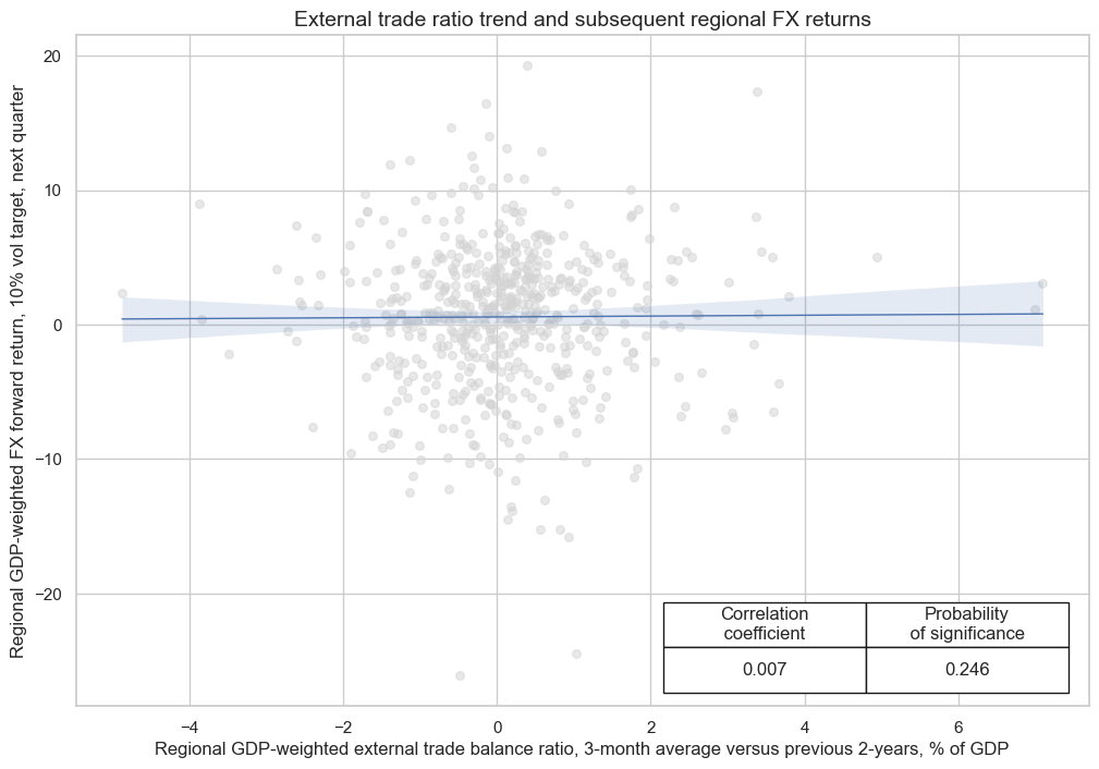
The use of regional baskets of signals and returns can be very useful if there is “leakage” of country economic and return trends across currency areas that are similar, be it geographic or otherwise. For example, a deterioration in external balances in some countries may increase the risk of setbacks in regional FX returns or returns for a set of currency areas with similar properties.
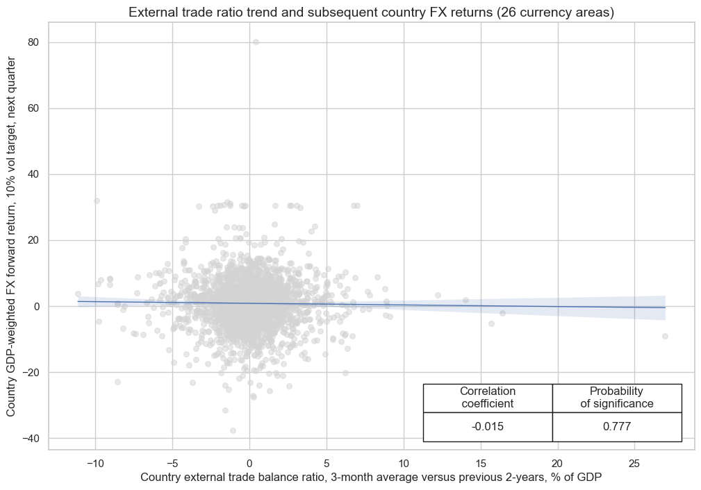
The below analysis looks at the correlation trends in external trade balance ratios and subsequent FX returns. It shows that the formation of GDP-weighted similar groups of countries helps to find a significant relation that is not easily visible on a country-by-country basis or a general currency area panel.
# FX trading regions

cids_defx = ["CHF", "GBP", "NOK", "SEK"]  # DM Europe
cids_dcfx = ["AUD", "CAD", "NZD"]  # DM commodity
cids_eefx = ["CZK", "HUF", "PLN", "RON"]  # EM EU
cids_lafx = ["BRL", "COP", "CLP", "MXN", "PEN"]  # Latam
cids_eafx = ["RUB", "TRY", "ZAR"]  # EMEA
cids_asfx = ["IDR", "INR", "KRW", "MYR", "PHP", "THB", "TWD"]  # EM Asia

cids_fx = cids_defx + cids_dcfx + cids_eefx + cids_lafx + cids_eafx + cids_asfx

# Weighted baskets

xcatx = ["FXXR_VT10", "MTBGDPRATIO_SA_3MMAv24MMA"]  # ["FXXR_VT10", "FXCRR_VT10"]
baskets = {
    "DM_EU": cids_defx,
    "DM_CO": cids_dcfx,
    "EM_EU": cids_eefx,
    "EM_LA": cids_lafx,
    "EM_AS": cids_asfx,
    "EM_EA": cids_eafx,
}
dfx = dfd.copy()

for xc in xcatx:
    for key, value in baskets.items():
        dfa = msp.linear_composite(
            dfx,
            xcats=xc,
            cids=value,
            weights="USDGDPWGT_SA_3YMA",
            new_cid=key,
            complete_cids=False,
        )
        dfx = msm.update_df(dfx, dfa)
cr = msp.CategoryRelations(
    dfx,
    xcats=["MTBGDPRATIO_SA_3MMAv24MMA", "FXXR_VT10"],  # ["FXCRR_VT10", "FXXR_VT10"],
    cids=[key for key in baskets.keys()],
    freq="Q",
    lag=1,
    xcat_aggs=["last", "sum"],
    fwin=1,
    start="2000-01-01",
    years=None,
)

cr.reg_scatter(
    title=f"External trade ratio trend and subsequent regional FX returns",
    labels=False,
    coef_box="lower right",
    xlab="Regional GDP-weighted external trade balance ratio, 3-month average versus previous 2-years, % of GDP",
    ylab="Regional GDP-weighted FX forward return, 10% vol target, next quarter",
    prob_est="map",
)

cr = msp.CategoryRelations(
    dfx,
    xcats=["MTBGDPRATIO_SA_3MMAv24MMA", "FXXR_VT10"],  # ["FXCRR_VT10", "FXXR_VT10"],
    cids=cids_fx,
    freq="Q",
    lag=1,
    xcat_aggs=["last", "sum"],
    fwin=1,
    start="2000-01-01",
    years=None,
)

cr.reg_scatter(
    title=f"External trade ratio trend and subsequent country FX returns (26 currency areas)",
    labels=False,
    coef_box="lower right",
    xlab="Country external trade balance ratio, 3-month average versus previous 2-years, % of GDP",
    ylab="Country GDP-weighted FX forward return, 10% vol target, next quarter",
    prob_est="map",
)

Appendices #
Appendix 1: Currency symbols #
The word ‘cross-section’ refers to currencies, currency areas or economic areas. In alphabetical order, these are AUD (Australian dollar), BRL (Brazilian real), CAD (Canadian dollar), CHF (Swiss franc), CLP (Chilean peso), CNY (Chinese yuan renminbi), COP (Colombian peso), CZK (Czech Republic koruna), DEM (German mark), ESP (Spanish peseta), EUR (Euro), FRF (French franc), GBP (British pound), HKD (Hong Kong dollar), HUF (Hungarian forint), IDR (Indonesian rupiah), ITL (Italian lira), JPY (Japanese yen), KRW (Korean won), MXN (Mexican peso), MYR (Malaysian ringgit), NLG (Dutch guilder), NOK (Norwegian krone), NZD (New Zealand dollar), PEN (Peruvian sol), PHP (Phillipine peso), PLN (Polish zloty), RON (Romanian leu), RUB (Russian ruble), SEK (Swedish krona), SGD (Singaporean dollar), THB (Thai baht), TRY (Turkish lira), TWD (Taiwanese dollar), USD (U.S. dollar), ZAR (South African rand).


