Producer price inflation surprises

This category contains economic surprise indicators related to producer price inflation . Quantamental surprises measure the difference between realised inflation data and model-implied expectations formed using only information available before the release — a proxy for what the market might reasonably have expected at the time. They provide a systematic view of inflation surprises, defined as deviations from credible real-time forecasts.

For detailed methodology on surprise construction, including transformation logic and real-time forecast design, see Appendix 2 and the research article Quantamental economic surprise indicators: a primer .

Suprises to annual inflation rates

Ticker : PPIH_NSA_P1M1ML12_ARMAS / _P1M1ML12_3MMA_ARMAS / PPIH_NSA_P1Q1QL4_ARMAS

Label : Producer price index ARMA(1,1)-based surprises: %oya / %oya, 3mma / %oya (q)

Definition : Producer price index ARMA(1,1)-based surprises: % over a year ago / % over a year ago, 3-month moving average / % over a year ago (quarterly)

Notes :

• Refer to the section on standard PPI inflation

• Expected values are derived from the one-step-ahead forecast produced by the previous vintage of a univariate ARMA(1,1) time series model. This model predicts monthly log-changes of the price index, based on the previous month’s value (autoregressive component) and the most recent model residual (i.e. the in-sample error used in the moving average component). These forecasts are applied to the price index to construct the expected year-over-year inflation rate.

• Model coefficients are estimated separately for each data vintage, using only the information available at that point in time. This ensures every forecast is genuinely out-of-sample, reflecting expectations based on real-time data.

• Surprises are calculated as the difference between the actual and forecasted value of the year-over-year percentage change in the relevant producer price index. In the case of pure revisions, without release of a new observation period, the surprise is the difference between the pre-release and post-release inflation rate.

Surprises to short-term seasonally-adjusted PPI trends

Ticker : PPIH_SA_P3M3ML3AR_ARMAS / _P6M6ML6AR_ARMAS / P1Q1QL1AR_ARMAS / _P2Q2QL2AR_ARMAS

Label : Producer price index ARMA(1,1)-based surprises: % 3m/3m ar / % 6m/6m ar / % q/q ar / % 2q/2q ar

Definition : Producer price index ARMA(1,1)-based surprises: % 3 months over previous 3 months, annualized / % 6 months over previous 6 months, annualized / % quarter over previous quarter, annualized / % 2 quarters over previous 2 quarters, annualized

Notes :

• Refer to the section on seasonally-adjusted PPI trends

• Expected values are derived from the one-step-ahead forecast produced by the previous vintage of a univariate ARMA(1,1) time series model. This model predicts monthly log-changes of the price index, based on the previous month’s value (autoregressive component) and the most recent model residual (i.e. the in-sample error used in the moving average component). These forecasts are applied to the price index to construct the expected inflation trend.

• Model coefficients are estimated separately for each data vintage, using only the information available at that point in time. This ensures every forecast is genuinely out-of-sample, reflecting expectations based on real-time data.

• Surprises are calculated as the difference between the actual and forecasted value of the year-over-year percentage change in the relevant producer price index. In the case of pure revisions, without release of a new observation period, the surprise is the difference between the pre-release and post-release inflation rate.

Imports

Only the standard Python data science packages and the specialized macrosynergy package are needed.

import os
import pandas as pd
import matplotlib.pyplot as plt
import numpy as np

import macrosynergy.management as msm
import macrosynergy.panel as msp
import macrosynergy.signal as mss
import macrosynergy.pnl as msn
import macrosynergy.visuals as msv

from macrosynergy.download import JPMaQSDownload

import warnings
warnings.simplefilter("ignore")

The JPMaQS indicators we consider are downloaded using the J.P. Morgan Dataquery API interface within the macrosynergy package. This is done by specifying ticker strings , formed by appending an indicator category code <category> to a currency area code <cross_section> . These constitute the main part of a full quantamental indicator ticker, taking the form DB(JPMAQS,<cross_section>_<category>,<info>) , where <info> denotes the time series of information for the given cross-section and category. The following types of information are available:

• value giving the latest available values for the indicator

• eop_lag referring to days elapsed since the end of the observation period

• mop_lag referring to the number of days elapsed since the mean observation period

• grade denoting a grade of the observation, giving a metric of real time information quality.

After instantiating the JPMaQSDownload class within the macrosynergy.download module, one can use the download(tickers,start_date,metrics) method to easily download the necessary data, where tickers is an array of ticker strings, start_date is the first collection date to be considered and metrics is an array comprising the times series information to be downloaded.

# Cross-sections of interest

cids_dmca = [
    "AUD",
    "CAD",
    "CHF",
    "EUR",
    "GBP",
    "JPY",
    "NOK",
    "NZD",
    "SEK",
    "USD",
]  # DM currency areas
cids_dmec = ["DEM", "ESP", "FRF", "ITL", "NLG"]  # DM euro area countries

cids_dm = cids_dmca + cids_dmec

cids_em = [
    "BRL",  # Latam
    "COP",
    "CLP",
    "MXN",
    "PEN",
    "CZK",  # EMEA
    "HUF",
    "ILS",
    "PLN",
    "RON",
    "RUB",
    "TRY",
    "ZAR", 
    "CNY",  # Asia
    "IDR",
    "INR",
    "KRW",
    "MYR",
    "PHP",
    "SGD",
    "THB",
    "TWD",
] 

cids_early = ["GBP", "JPY", "USD", "RUB", "TRY", "ZAR", "PHP", "SGD"]

cids = sorted(cids_dm + cids_em)
# Exported selection for further use
cids_exp = cids

# Quantamental categories of interest

main = []

# PPI  over a year ago
for base in ["PPIH_NSA"]:
    for transform in ("P1M1ML12", "P1Q1QL4", "P1M1ML12_3MMA"):
        main.append(f"{base}_{transform}_ARMAS")


# PPI trends
for base in ["PPIH_SA"]:
    for transform in ("P1Q1QL1AR", "P2Q2QL2AR", "P3M3ML3AR", "P6M6ML6AR"):
        main.append(f"{base}_{transform}_ARMAS")


# Economic context variables
econ = [
    "RIR_NSA",
    "IVAWGT_SA_1YMA",
    "PPIH_NSA_P1M1ML12"
]

# Market-linked context variables
mark = [
    "FXXR_NSA", "FXXR_VT10",
    "DU02YXR_NSA", "DU02YXR_VT10",
    "DU05YXR_NSA", "DU05YXR_VT10",
    "FXUNTRADABLE_NSA", "FXTARGETED_NSA",
    "EQXR_VT10",
    "DU05YXR_NSA",
    "DU05YXR_VT10",
    "DU10YXR_VT10",
]

# Combined list of cross-sectional categories
xcats = main + econ + mark

# Download series from J.P. Morgan DataQuery by tickers

start_date = "1990-01-01"
tickers = [cid + "_" + xcat for cid in cids for xcat in xcats]
print(f"Maximum number of tickers is {len(tickers)}")

# Retrieve credentials

client_id: str = os.getenv("DQ_CLIENT_ID")
client_secret: str = os.getenv("DQ_CLIENT_SECRET")

with JPMaQSDownload(client_id=client_id, client_secret=client_secret) as dq:
    df = dq.download(
        tickers=tickers,
        start_date=start_date,
        suppress_warning=True,
        metrics=["all"],
        show_progress=True,
    )
    # Store downloaded DataFrame
dfd = df

Maximum number of tickers is 814
Downloading data from JPMaQS.
Timestamp UTC:  2025-08-19 14:37:41
Connection successful!

Requesting data: 100%|██████████| 185/185 [00:38<00:00,  4.83it/s]
Downloading data: 100%|██████████| 185/185 [01:07<00:00,  2.73it/s]

Some expressions are missing from the downloaded data. Check logger output for complete list.
970 out of 3700 expressions are missing. To download the catalogue of all available expressions and filter the unavailable expressions, set `get_catalogue=True` in the call to `JPMaQSDownload.download()`.

Availability

# Define subset of cross-sections and key indicator categories for availability check

cidx = cids_exp  # Use all cross-sections previously defined

xcatx = [
    "PPIH_NSA_P1M1ML12_ARMAS",    # PPIH, % oya
    "PPIH_NSA_P1Q1QL4_ARMAS",    # PPIH, % oya
]

# Run availability check on selected indicators and cross-sections
msm.check_availability(
    df=dfd,
    xcats=xcatx,
    cids=cidx,
    missing_recent=False,
)

Show code cell output

Hide code cell output

Real-time quantamental indicators of producer price inflation trends have typically been available for developed markets since the late 1990s. For many emerging markets, data start from around 2000. For an explanation of the currency codes, which refer to currency areas or countries with available categories, see Appendix 1 .

The chart below shows the average vintage grades of PPI surprise indicators across countries. Grading reflects the timeliness and quality of real-time data available for each series since the start date.

Vintage quality looks to be low with only AUD and DEM to have grades less then two.

xcatx = [
    "PPIH_NSA_P1M1ML12_ARMAS",    # PPIH, % oya
    "PPIH_NSA_P1Q1QL4_ARMAS",    # PPIH, % oya
]

cidx = cids_exp

plot = msp.heatmap_grades(
    dfd,
    xcats=xcatx,
    cids=cidx,
    size=(18, 1),
    title=f"Average vintage grades from {start_date} onwards",
    start=start_date,
)

The distribution below shows end-of-observation period lags. Poland data was yearly early on explaining the consistent long lags.

# View eop_lag ranges by cross-section for selected PPI surprise indicators

cidx = cids
xcatx = [
    "PPIH_NSA_P1M1ML12_ARMAS",    # PPIH, % oya
    "PPIH_NSA_P1Q1QL4_ARMAS",    # PPIH, % oya
]

for xcat in xcatx:
    msp.view_ranges(
        dfd,
        xcats=[xcat],
        cids=cidx,
        val="eop_lag",
        title=f"{xcat}: End-of-observation-period lag (days)",
        start="2000-01-01",
        kind="box",
        size=(16, 4),
    )

# Rename quarterly categories for simplified charting

dict_repl = {
    "PPIH_NSA_P1Q1QL4_ARMAS": "PPIH_NSA_P1M1ML12_ARMAS",
    "PPIH_SA_P1Q1QL1AR_ARMAS": "PPIH_SA_P3M3ML3AR_ARMAS",
    "PPIH_SA_P2Q2QL2AR_ARMAS": "PPIH_SA_P6M6ML6AR_ARMAS",
}

# Replace only exact matches for xcat names
dfd["xcat"] = dfd["xcat"].replace(dict_repl)

History

The variance of PPI inflation surprises has been very different across countries, reflecting differences in the types of locally produced goods and the variability of the exchange rates. It will often be necessary to normalize surprises based on local standard deviations.

# Boxplots of headline PPI surprise distributions (seasonally adjusted), by country

xcatx = ["PPIH_NSA_P1M1ML12_ARMAS"]


cids_filtered = sorted(set(cids_exp) - {"PEN"})

msp.view_ranges(
    dfd,
    xcats=xcatx,
    cids=cids_filtered,
    sort_cids_by="std",
    start=start_date,
    kind="bar",
    title="Distribution of headline PPI surprises, by country",
    size=(16, 8),
)

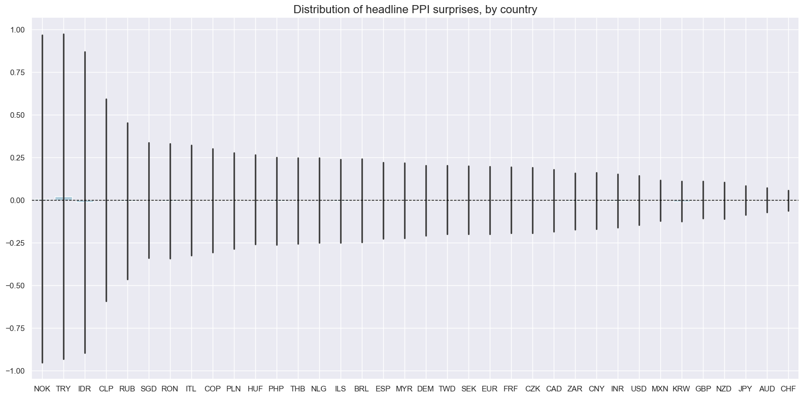
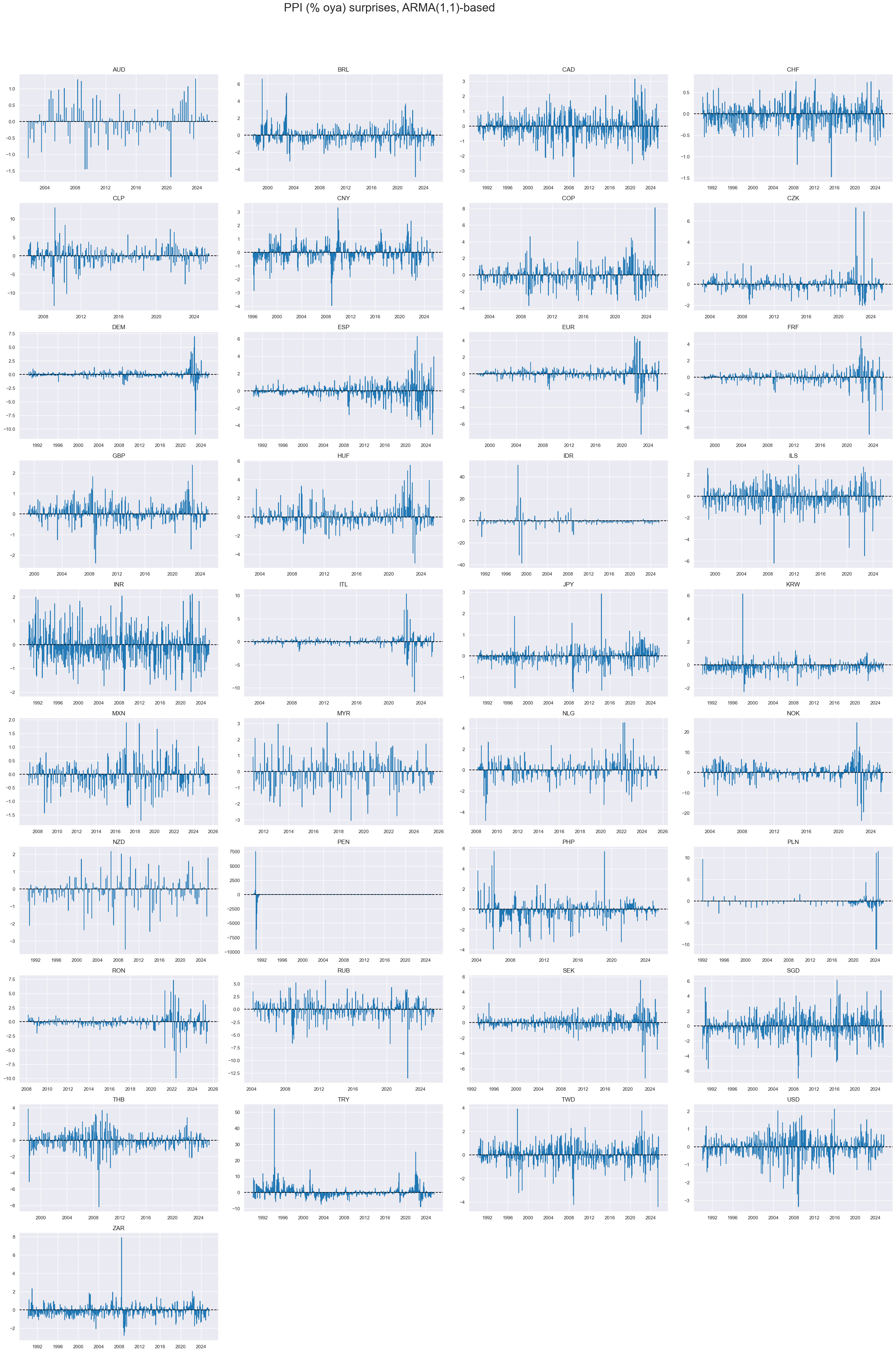
A few countries (Indonesia, Peru and Turkey) experienced periods of very high PPI inflation. These also gave rise to huge “surprises” in percentage terms.

# Timeline plots of headline inflation levels vs. inflation surprises
# Focus on countries with more volatile or non-stationary inflation dynamics

xcatx = [
    "PPIH_NSA_P1M1ML12",          
    "PPIH_NSA_P1M1ML12_ARMAS"     
]

cidx = ["PEN","IDR","TRY"]

msp.view_timelines(
    dfd,
    xcats=xcatx,
    cids=cidx,
    start=start_date,
    title="PPI inflation and estimated surprises",
    title_adj=1.02,
    title_xadj=0.435,
    title_fontsize=27,
    legend_fontsize=17,
    label_adj=0.075,
    ncol=3,
    same_y=False,
    size=(12, 7),
    aspect=1.7,
    all_xticks=True,
)

xcatx = ["PPIH_NSA_P1M1ML12_ARMAS"]

# Use all available cross-sections
cidx = sorted(cids_exp)

msp.view_timelines(
    dfd,
    xcats=xcatx,
    cids=cidx,
    start=start_date,
    title="PPI (% oya) surprises, ARMA(1,1)-based",
    title_adj=1.02,
    title_xadj=0.435,
    title_fontsize=27,
    legend_fontsize=17,
    label_adj=0.075,
    ncol=4,
    same_y=False,
    size=(12, 7),
    aspect=1.7,
    all_xticks=True,
)

# Timelines of core PPI surprises (% oya), ARMA(1,1)-based
# Excluding PEN due to limited or unreliable coverage

xcatx = ["PPIH_SA_P3M3ML3AR_ARMAS"]

cidx = sorted(set(cids_exp) - {"CNY"})

msp.view_timelines(
    dfd,
    xcats=xcatx,
    cids=cidx,
    start=start_date,
    title="Short-term PPI trend (% 3m/3m, saar) surprises, ARMA(1,1)-based",
    title_adj=1.02,
    title_xadj=0.435,
    title_fontsize=27,
    legend_fontsize=17,
    label_adj=0.075,
    ncol=4,
    same_y=False,
    size=(12, 7),
    aspect=1.7,
    all_xticks=True,
)

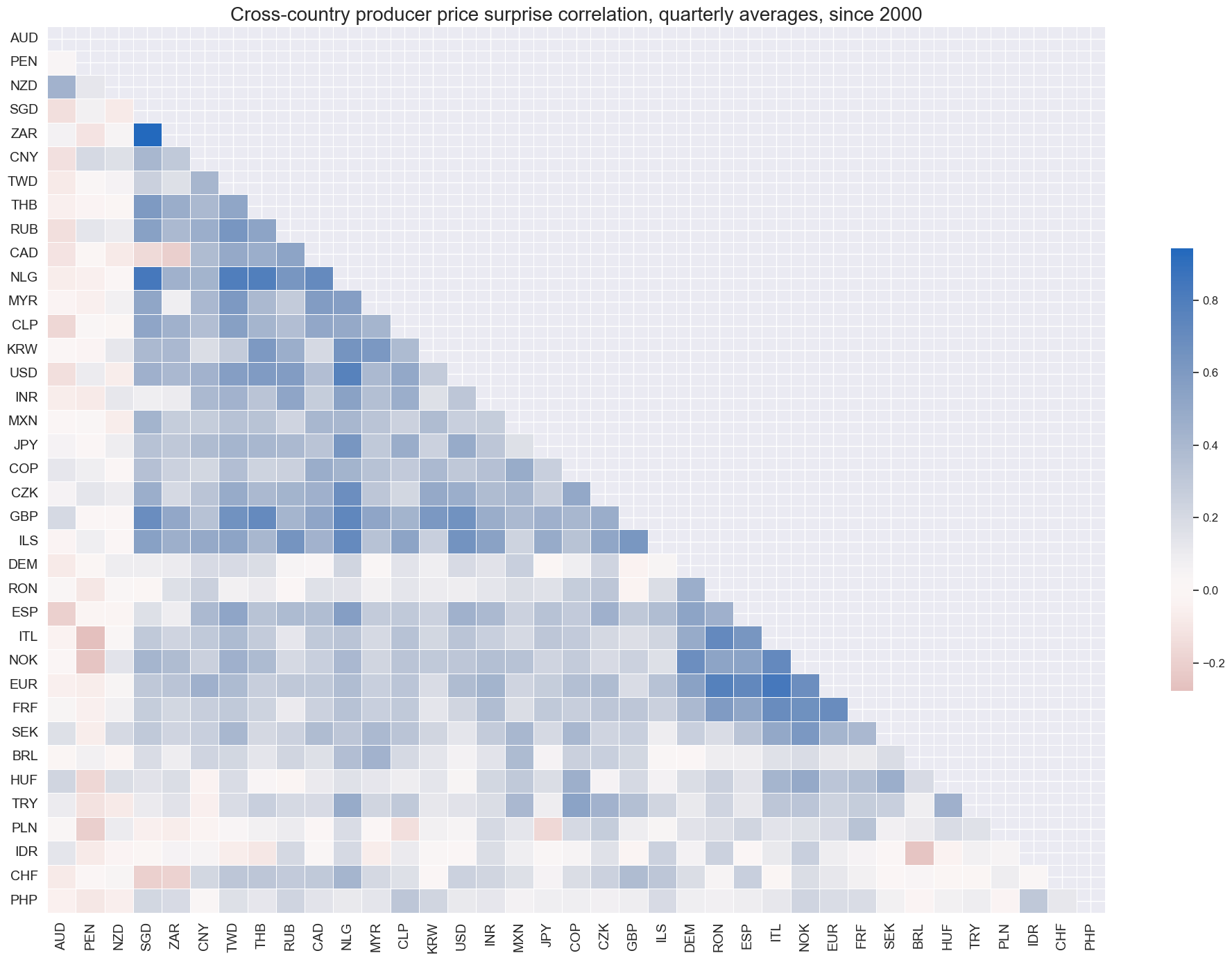
Based on quarterly averages, inflation surprises have been mostly positively correlated internationally. Those countries with no or negative correlation have published data at quarterly, rather than monthly, frequencies.

cidx = cids
msp.correl_matrix(
    dfd,
    xcats="PPIH_NSA_P1M1ML12_ARMAS",
    cids=cidx,
    freq="q",
    title="Cross-country producer price surprise correlation, quarterly averages, since 2000",
    cluster=True,
    size=(20, 14),
)

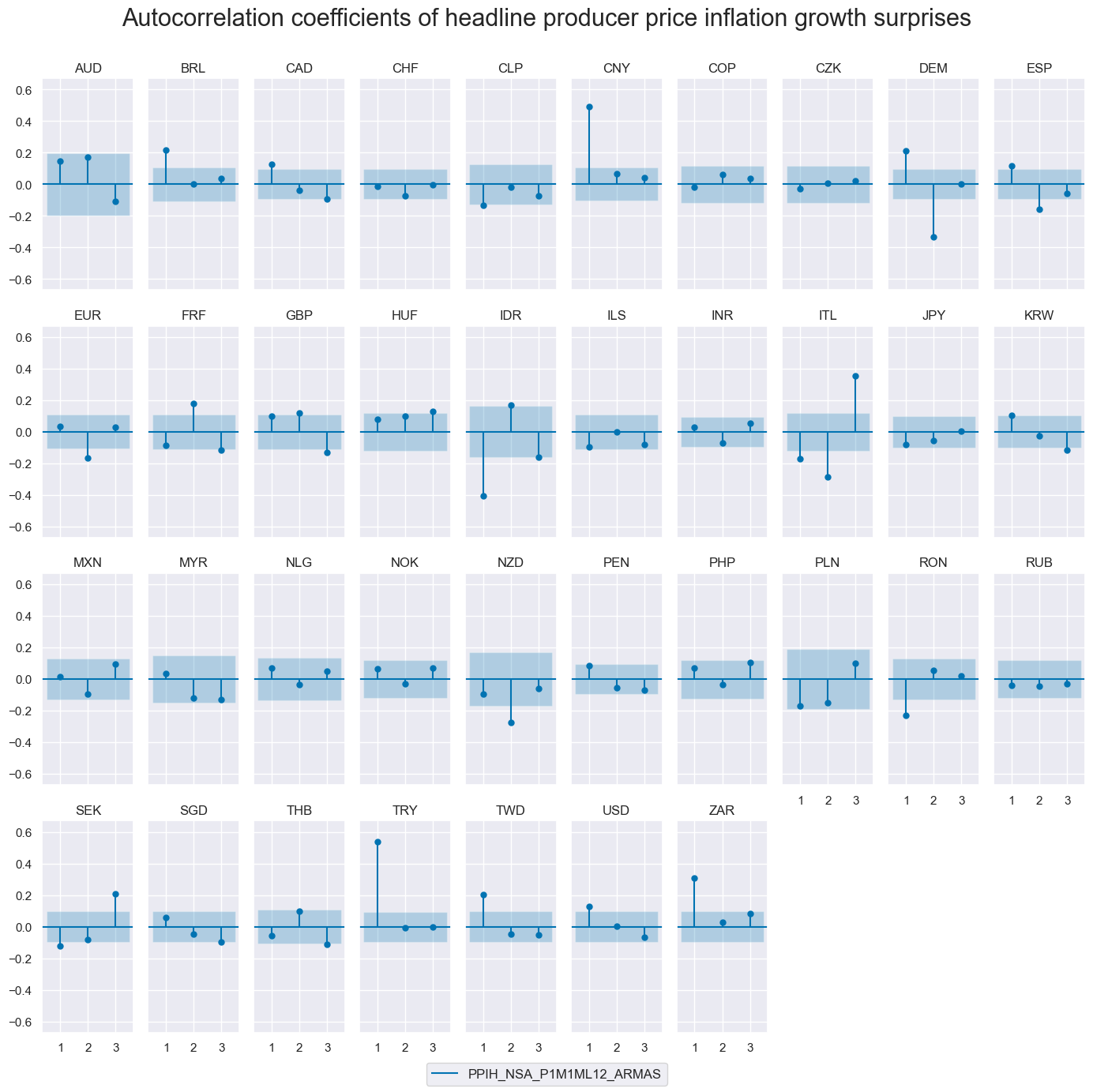
The autocorrelation (ACF) plots assess whether PPI surprise series exhibit temporal dependence. Under the assumption of a well-specified, unbiased one-step-ahead forecast model, real-time surprises should show no systematic autocorrelation.

Most countries conform to this expectation. However, a few — such as China and Turkey — exhibit residual autocorrelation, likely reflecting episodes of structural inflation shifts or prolonged non-stationarity that challenge the assumptions of the ARMA model.

# Plot PACF of headline PPI surprise series (% oya), ARMA(1,1)-based

cidx = sorted(cids_exp)

msv.plot_pacf(
    df=dfd,
    cids=cidx,
    xcat="PPIH_NSA_P1M1ML12_ARMAS",
    title="Autocorrelation coefficients of headline producer price inflation growth surprises",
    lags=3,
    remove_zero_predictor=True,
    figsize=(14, 14),
    ncols=10,
)

Importance

Research links

No research related to this category group was found so far.

Empirical clues

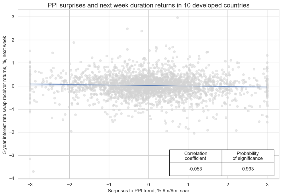
Unexpectedly strong PPI growth is usually bad news for duration exposure as it points to both inflation pressure and stronger corporate earnings growth, both of which justify higher interest rates.Empirically, normalized headline PPI inflation surprises have been significant negative predictors for next week duration returns, as indicated by 5-year or 10-year IRS fixed receiver returns.

# Construct normalised inflation surprise indicators from consistent PPI trend metrics

xcatx = [

    "PPIH_NSA_P1M1ML12_ARMAS",       # Headline PPI, monthly trend surprise
    "PPIH_SA_P3M3ML3AR_ARMAS",     # Headline PPI, 3-month adjusted trend surprise
    "PPIH_SA_P6M6ML6AR_ARMAS",     # Headline PPI, 6-month adjusted trend surprise

]

# Filter cross-sections (excluding Peru)
cidx = list(set(cids_exp) - set(["PEN"]))

# Reduce dataframe to relevant categories and countries
df_red = msm.reduce_df(dfd, xcats=xcatx, cids=cidx)

# Transform to z-scored information state change indicators (standardised surprise signal)
isc_obj = msm.InformationStateChanges.from_qdf(df=df_red, score_by="level")
dfa = isc_obj.to_qdf(value_column="zscore", postfix="N")

# Cap extreme values to +/- 3 standard deviations
dfa["value"] = dfa["value"].clip(lower=-3, upper=3)

# Update main dataframe with the new signals
dfd = msm.update_df(dfd, dfa[["real_date", "cid", "xcat", "value"]])

cr = msp.CategoryRelations(
    dfd,
    xcats=["PPIH_SA_P6M6ML6AR_ARMASN", "DU05YXR_NSA"],  # Headline PPI surprise and 5Y IRS receiver return
    cids=cids_dmca,                                     # Developed market countries
    freq="w",                                           
    lag=1,                                              
    xcat_aggs=["sum", "sum"],                          
    fwin=1,
    start="2000-01-01",
    years=None,
)

cr.reg_scatter(
    title="PPI surprises and next week duration returns in 10 developed countries",
    title_fontsize=16,
    labels=False,
    coef_box="lower right",
    xlab="Surprises to PPI trend, % 6m/6m, saar",
    ylab="5-year interest rate swap receiver returns, %, next week",
    remove_zero_predictor=True,
    size=(10, 7)
)