Private consumption surprises #
This category group contains economic surprise indicators related to private consumption growth, retail sales growth, and consumer confidence indicators. Economic surprises are deviations of point-in-time quantamental indicators from predicted values. For an in-depth explanation, please read Appendix 2 .
Private consumption growth surprises #
Ticker : RPCONS_SA_P1Q1QL4_ARMAS / RPCONS_SA_P1M1ML12_ARMAS / RPCONS_SA_P1M1ML12_3MMA_ARMAS
Label : Real Private consumption, sa: % oya (q), ARMA(1,1)-based surprises / % oya, ARMA(1,1)-based surprises / % oya, 3mma, ARMA(1,1)-based surprises
Definition : Real Private consumption, seasonally adjusted: percentage over a year ago (quarterly), ARMA(1,1)-based surprises / percentage over a year ago, ARMA(1,1)-based surprises / percentage over a year ago, 3-month moving average, ARMA(1,1)-based surprises
Notes :
-
Refer to the section on private consumption growth for notes on the underlying data series.
-
Expected values for release dates are based on an “ARMA(1,1)” model. This is a simple univariate time series model that predicts increments based on an autoregressive component, i.e., last period’s value, and a moving average component, represented by last period’s error. The coefficients of the model are estimated sequentially based on the vintages of the underlying data. And each vintage-specific model produces a one-step-ahead forecast for the subsequent observation period.
Private consumption trend surprises #
Ticker : RPCONS_SA_P1Q1QL1AR_ARMAS / RPCONS_SA_P2Q2QL2AR_ARMAS / RPCONS_SA_P3M3ML3AR_ARMAS / RPCONS_SA_P6M6ML6AR_ARMAS
Label : Real Private consumption, sa: % 1q/1q ar, ARMA(1,1)-based surprises / % 2q/2q ar, ARMA(1,1)-based surprises / % 3m/3m ar, ARMA(1,1)-based surprises / % 6m/6m ar, ARMA(1,1)-based surprises
Definition : Real Private consumption, seasonally adjusted: % of latest quarter over previous quarter at annualized rate, ARMA(1,1)-based surprises / % of latest 2 quarters over previous 2 quarters at an annualized rate, ARMA(1,1)-based surprises / % of latest 3 months over previous 3 months at annualized rate, ARMA(1,1)-based surprises / % of latest 6 months over previous 6 months at an annualized rate, ARMA(1,1)-based surprises
Notes :
-
Refer to the section on private consumption trends for notes on the underlying data series.
-
Expected values for release dates are based on an “ARMA(1,1)” model. This is a simple univariate time series model that predicts increments based on an autoregressive component, i.e., last period’s value, and a moving average component, represented by last period’s error. The coefficients of the model are estimated sequentially based on the vintages of the underlying data. And each vintage-specific model produces a one-step-ahead forecast for the subsequent observation period.
Consumer confidence score surprises #
Ticker : CCSCORE_SA_ARMAS / CCSCORE_SA_3MMA_ARMAS
Label : Consumer confidence, sa: z-score, ARMA(1,1)-based surprises / z-score, 3mma, ARMA(1,1)-based surprises
Definition : Consumer confidence, seasonally adjusted: z-score, ARMA(1,1)-based surprises / z-score, 3-month moving average, ARMA(1,1)-based surprises
Notes :
-
Refer to the section on consumer confidence scores for notes on the underlying data series.
-
Expected values for release dates are based on an “ARMA(1,1)” model. This is a simple univariate time series model that predicts increments based on an autoregressive component, i.e., last period’s value, and a moving average component, represented by last period’s error. The coefficients of the model are estimated sequentially based on the vintages of the underlying data. And each vintage-specific model produces a one-step-ahead forecast for the subsequent observation period.
-
The methodology for the US, for which there are two sources of data, is described in Appendix 3 .
Consumer confidence score trend surprises #
Ticker : CCSCORE_SA_D1M1ML1_ARMAS / CCSCORE_SA_D3M3ML3_ARMAS / CCSCORE_SA_D1Q1QL1_ARMAS / CCSCORE_SA_D6M6ML6_ARMAS / CCSCORE_SA_D2Q2QL2_ARMAS / CCSCORE_SA_D1M1ML12_ARMAS / CCSCORE_SA_3MMA_D1M1ML12_ARMAS / CCSCORE_SA_D1Q1QL4_ARMAS
Label : Consumer confidence, sa, z-score: diff m/m, ARMA(1,1)-based surprises / diff 3m/3m, ARMA(1,1)-based surprises / diff q/q, ARMA(1,1)-based surprises / diff 6m/6m, ARMA(1,1)-based surprises / diff 2q/2q, ARMA(1,1)-based surprises / diff oya (m), ARMA(1,1)-based surprises / diff oya, 3mma, ARMA(1,1)-based surprises / diff oya (q), ARMA(1,1)-based surprises
Definition : Consumer confidence, seasonally adjusted, z-score: difference over 1 month, ARMA(1,1)-based surprises / difference of last 3 months over previous 3 months, ARMA(1,1)-based surprises / difference of last quarter over previous quarter, ARMA(1,1)-based surprises / difference of last 6 months over previous 6 months, ARMA(1,1)-based surprises / difference of last 2 quarters over previous 2 quarters, ARMA(1,1)-based surprises / difference over a year ago, monthly values, ARMA(1,1)-based surprises / difference over a year ago, 3-month moving average, ARMA(1,1)-based surprises / difference over a year ago, quarterly values, ARMA(1,1)-based surprises
Notes :
-
Refer to the section on consumer confidence scores trends for notes on the underlying data series.
-
Expected values for release dates are based on an “ARMA(1,1)” model. This is a simple univariate time series model that predicts increments based on an autoregressive component, i.e., last period’s value, and a moving average component, represented by last period’s error. The coefficients of the model are estimated sequentially based on the vintages of the underlying data. And each vintage-specific model produces a one-step-ahead forecast for the subsequent observation period.
-
The methodology for the US, for which there are two sources of data, is described in Appendix 3 .
Retail sales growth surprises #
Ticker : NRSALES_SA_P1M1ML12_ARMAS / NRSALES_SA_P1M1ML12_3MMA_ARMAS / NRSALES_SA_P1Q1QL4_ARMAS
Label : Nominal retail sales, sa: % oya, ARMA(1,1)-based surprises / % oya, 3mma, ARMA(1,1)-based surprises / % oya (q), ARMA(1,1)-based surprises
Definition : Nominal retail sales, seasonally adjusted: percentage over a year ago, ARMA(1,1)-based surprises / percentage over a year ago, 3-month moving average, ARMA(1,1)-based surprises / percentage over a year ago (quarterly), ARMA(1,1)-based surprises
Notes :
-
Refer to the section on retail sales growth for notes on the underlying data series.
-
Expected values for release dates are based on an “ARMA(1,1)” model. This is a simple univariate time series model that predicts increments based on an autoregressive component, i.e., last period’s value, and a moving average component, represented by last period’s error. The coefficients of the model are estimated sequentially based on the vintages of the underlying data. And each vintage-specific model produces a one-step-ahead forecast for the subsequent observation period.
Ticker : RRSALES_SA_P1M1ML12 / RRSALES_SA_P1M1ML12_3MMA / RRSALES_SA_P1Q1QL4
Label : Real retail sales, sa: % oya, ARMA(1,1)-based surprises / % oya, 3mma, ARMA(1,1)-based surprises / % oya (q), ARMA(1,1)-based surprises
Definition : Real retail sales, seasonally adjusted: percentage over a year ago, ARMA(1,1)-based surprises / percentage over a year ago, 3-month moving average, ARMA(1,1)-based surprises / percentage over a year ago (quarterly), ARMA(1,1)-based surprises
Notes :
-
Refer to the section on retail sales growth for notes on the underlying data series.
-
Expected values for release dates are based on an “ARMA(1,1)” model. This is a simple univariate time series model that predicts increments based on an autoregressive component, i.e., last period’s value, and a moving average component, represented by last period’s error. The coefficients of the model are estimated sequentially based on the vintages of the underlying data. And each vintage-specific model produces a one-step-ahead forecast for the subsequent observation period.
Imports #
Only the standard Python data science packages and the specialized
macrosynergy
package are needed.
import os
import numpy as np
import pandas as pd
import matplotlib.pyplot as plt
import seaborn as sns

import macrosynergy.management as msm
import macrosynergy.panel as msp
import macrosynergy.signal as mss
import macrosynergy.pnl as msn
import macrosynergy.visuals as msv

from macrosynergy.download import JPMaQSDownload

from timeit import default_timer as timer
from datetime import timedelta, date, datetime

import warnings

warnings.simplefilter("ignore")
The
JPMaQS
indicators are retrieved using the J.P. Morgan DataQuery API via the
macrosynergy
package. Tickers are constructed by combining a currency area code (
<cross_section>
) with an indicator category code (
<category>
), forming a string of the form
<cross_section>_<category>
.
This composite string is embedded within a full DataQuery ticker:
DB(JPMAQS,<cross_section>_<category>,<info>)
where
<info>
refers to the type of time series data requested. The available options are:
-
value: the latest available value of the indicator -
eop_lag: days since the end of the observation period -
mop_lag: days since the mean observation period -
grade: a real-time data quality metric
To download data, instantiate the
JPMaQSDownload
class from
macrosynergy.download
, and use the
            .download(tickers,


            start_date,


            metrics)
method, where:
-
tickersis a list of constructed ticker strings -
start_dateis the first collection date to retrieve -
metricsspecifies the types of information (e.g.value,grade) to download
The
macrosynergy
package makes it easy to retrieve and work with this data in a fully programmatic and repeatable way.
# Cross-sections of interest

cids_dmca = ["AUD","CAD","CHF","EUR","GBP","JPY","NOK","NZD","SEK","USD"]  # DM currency areas
cids_dmec = ["DEM", "ESP", "FRF", "ITL", "NLG"]  # DM euro area countries
cids_latm = ["BRL", "COP", "CLP", "MXN", "PEN"]  # Latam countries
cids_emea = ["CZK", "HUF", "ILS", "PLN", "RON", "RUB", "TRY", "ZAR"]  # EMEA countries
cids_emas = ["CNY","HKD","IDR","INR","KRW","MYR","PHP","SGD","THB","TWD"]  # EM Asia countries

cids_dm = cids_dmca + cids_dmec
cids_em = cids_latm + cids_emea + cids_emas

cids = sorted(cids_dm + cids_em)

# FX cross-sections lists (for research purposes)

cids_nofx = ["EUR", "USD", "SGD"] + cids_dmec
cids_fx = list(set(cids) - set(cids_nofx))

cids_dmfx = set(cids_dm).intersection(cids_fx)
cids_emfx = set(cids_em).intersection(cids_fx)

cids_eur = ["CHF", "CZK", "HUF", "NOK", "PLN", "RON", "SEK"]  # trading against EUR
cids_eud = ["GBP", "RUB", "TRY"]  # trading against EUR and USD
cids_usd = list(set(cids_fx) - set(cids_eur + cids_eud))


cids_exp = sorted(list(set(cids) - set(cids_dmec)))  # cids expected in category panels excluding high yield and investment grade returns

# Sectorial equity index returns
cids_dmeq = ['AUD', 'CAD', 'CHF', 'EUR', 'GBP', 'HKD', 'ILS', 'JPY', 'NOK', 'NZD', 'SEK', 'SGD', 'USD']
cids_eueq = ["DEM", "ESP", "FRF", "ITL", "NLG"]

cids_rpcons = sorted(set(cids) - set(["CNY", "HKD"]))
cids_ccscore = sorted(set(cids) - set(['HKD', 'MYR', 'PEN', 'RON', 'SGD']))
# Quantamental categories of interest

xcats_ccscore = [
    f"CCSCORE_SA{transformation}_ARMAS" for transformation in
    [
        "",
        "_3MMA",
        "_D1M1ML1",
        "_D3M3ML3",
        "_D1Q1QL1",
        "_D6M6ML6",
        "_D2Q2QL2",
        "_3MMA_D1M1ML12",
        "_D1M1ML12",
        "_D1Q1QL4",
    ]]

xcats_nrsales = [
    f"NRSALES_SA{transformation}_ARMAS" for transformation in
    [
        "_P1M1ML12",
        "_P1M1ML12_3MMA",
        "_P1Q1QL4",
    ]]

xcats_rrsales = [
    f"RRSALES_SA{transformation}_ARMAS" for transformation in
    [
        "_P1M1ML12",
        "_P1M1ML12_3MMA",
        "_P1Q1QL4",
    ]]

xcats_rpcons = [
    f"RPCONS_SA{transformation}_ARMAS" for transformation in
    [
        "_P1M1ML12",
        "_P1M1ML12_3MMA",
        "_P1Q1QL4",
        "_P1Q1QL1AR",
        "_P2Q2QL2AR",
        "_P3M3ML3AR",
        "_P6M6ML6AR",
    ]]

main = xcats_ccscore + xcats_nrsales + xcats_rrsales + xcats_rpcons

mark = [
    "DU05YXR_NSA",
    "DU05YXR_VT10",
    "EQXR_NSA",
    "EQXR_VT10",
    "FXXR_NSA",
    "FXXR_VT10",
    "FXTARGETED_NSA",
    "FXUNTRADABLE_NSA",
]  # market links

xcats = main + mark
# Download series from J.P. Morgan DataQuery by tickers

start_date = "1990-01-01"

tickers = [cid + "_" + xcat for cid in cids for xcat in xcats]

print(f"Maximum number of tickers is {len(tickers)}")

# Retrieve credentials

client_id: str = os.getenv("DQ_CLIENT_ID")
client_secret: str = os.getenv("DQ_CLIENT_SECRET")

# Download from DataQuery

with JPMaQSDownload(client_id=client_id, client_secret=client_secret) as downloader:
    start = timer()
    df = downloader.download(
        tickers=tickers,
        start_date=start_date,
        metrics=["value", "eop_lag", "mop_lag", "grading"],
        suppress_warning=True,
        show_progress=True,
    )
    end = timer()


print("Download time from DQ: " + str(timedelta(seconds=end - start)))
Maximum number of tickers is 1178
Downloading data from JPMaQS.
Timestamp UTC:  2025-09-29 09:04:56
Connection successful!
Requesting data: 100%|██████████| 236/236 [00:50<00:00,  4.64it/s]
Downloading data: 100%|██████████| 236/236 [02:25<00:00,  1.62it/s]
Some expressions are missing from the downloaded data. Check logger output for complete list.
1928 out of 4712 expressions are missing. To download the catalogue of all available expressions and filter the unavailable expressions, set `get_catalogue=True` in the call to `JPMaQSDownload.download()`.
Download time from DQ: 0:03:28.212176
Availability #
For the explanation of currency symbols, which are related to currency areas or countries for which categories are available, please view Appendix 1 .
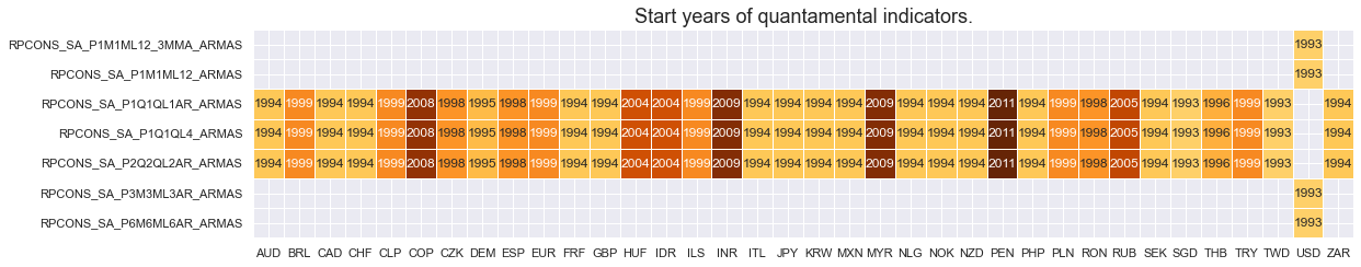
In most countries quantamental indicators of real private consumption surprises are available from the mid-1990s or early 2000s. For all but the U.S., countries have data available at a quarterly frequency.
xcatx = xcats_rpcons
cidx = cids

msm.check_availability(
    df,
    xcats=xcatx,
    cids=cidx,
    missing_recent=False,
)
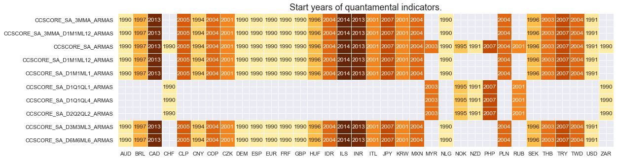
For the most part, consumer confidence score surprise indicators are available back to the early-1990s.
xcatx = xcats_ccscore
cidx = cids

msm.check_availability(
    df,
    xcats=xcatx,
    cids=cidx,
    missing_recent=False,
)
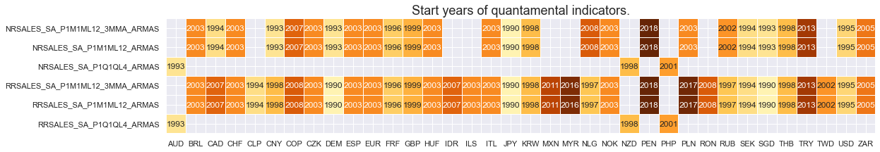
In most countries quantamental indicators of retail sales growth are available from the mid-1990s or early 2000s.
xcatx = xcats_nrsales + xcats_rrsales
cidx = cids

msm.check_availability(
    df,
    xcats=xcatx,
    cids=cidx,
    missing_recent=False,
)
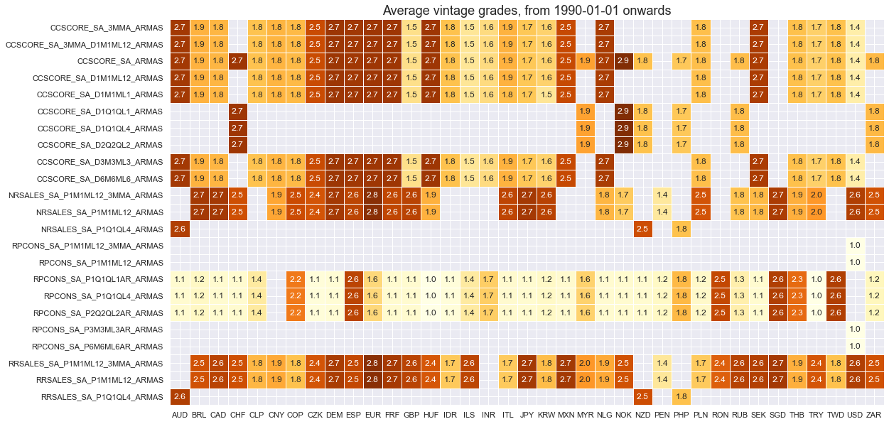
xcatx = main
cidx = cids

plot = msp.heatmap_grades(
    df,
    xcats=xcatx,
    cids=cidx,
    start=start_date,
    size=(18, 10),
    title=f"Average vintage grades, from {start_date} onwards",
)
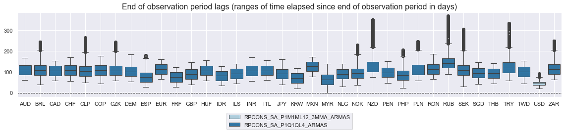
xcatx = ["RPCONS_SA_P1M1ML12_3MMA_ARMAS", "RPCONS_SA_P1Q1QL4_ARMAS"]
cidx = cids
msp.view_ranges(
    df,
    xcats=xcatx,
    cids=cidx,
    val="eop_lag",
    title="End of observation period lags (ranges of time elapsed since end of observation period in days)",
    start="2000-01-01",
    kind="box",
    size=(16, 4),
)
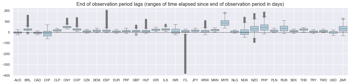
xcatx = ["CCSCORE_SA_ARMAS"]
cidx = cids
msp.view_ranges(
    df,
    xcats=xcatx,
    cids=cidx,
    val="eop_lag",
    title="End of observation period lags (ranges of time elapsed since end of observation period in days)",
    start="2000-01-01",
    kind="box",
    size=(16, 4),
)
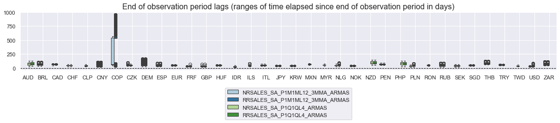
xcatx = ["NRSALES_SA_P1M1ML12_3MMA_ARMAS", "RRSALES_SA_P1M1ML12_3MMA_ARMAS", "NRSALES_SA_P1Q1QL4_ARMAS", "RRSALES_SA_P1Q1QL4_ARMAS"]
cidx = cids
msp.view_ranges(
    df,
    xcats=xcatx,
    cids=cidx,
    val="eop_lag",
    title="End of observation period lags (ranges of time elapsed since end of observation period in days)",
    start="2000-01-01",
    kind="box",
    size=(16, 4),
)
For graphical representation, it is helpful to rename some quarterly dynamics into an equivalent monthly dynamics.
dfx = df.copy()

dict_repl = {
    "CCSCORE_SA_D1Q1QL1_ARMAS": "CCSCORE_SA_D3M3ML3_ARMAS",
    "CCSCORE_SA_D2Q2QL2_ARMAS": "CCSCORE_SA_D6M6ML6_ARMAS",
    "CCSCORE_SA_D1Q1QL4_ARMAS": "CCSCORE_SA_3MMA_D1M1ML12_ARMAS",
    "NRSALES_SA_P1Q1QL4_ARMAS": "NRSALES_SA_P1M1ML12_3MMA_ARMAS",
    "RRSALES_SA_P1Q1QL4_ARMAS": "RRSALES_SA_P1M1ML12_3MMA_ARMAS",
    "RPCONS_SA_P1Q1QL4_ARMAS":  "RPCONS_SA_P1M1ML12_3MMA_ARMAS",
    "RPCONS_SA_P1Q1QL1AR_ARMAS":"RPCONS_SA_P3M3ML3AR_ARMAS",
    "RPCONS_SA_P2Q2QL2AR_ARMAS":"RPCONS_SA_P6M6ML6AR_ARMAS",

}

for key, value in dict_repl.items():
    dfx["xcat"] = dfx["xcat"].str.replace(key, value)
History #
Private consumption growth surprises #
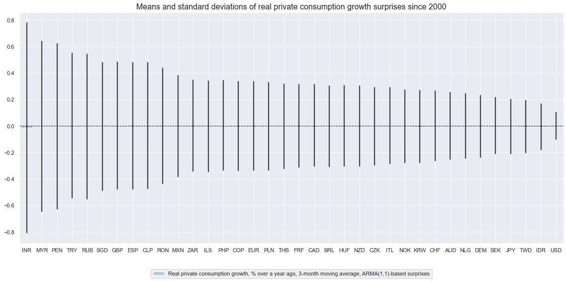
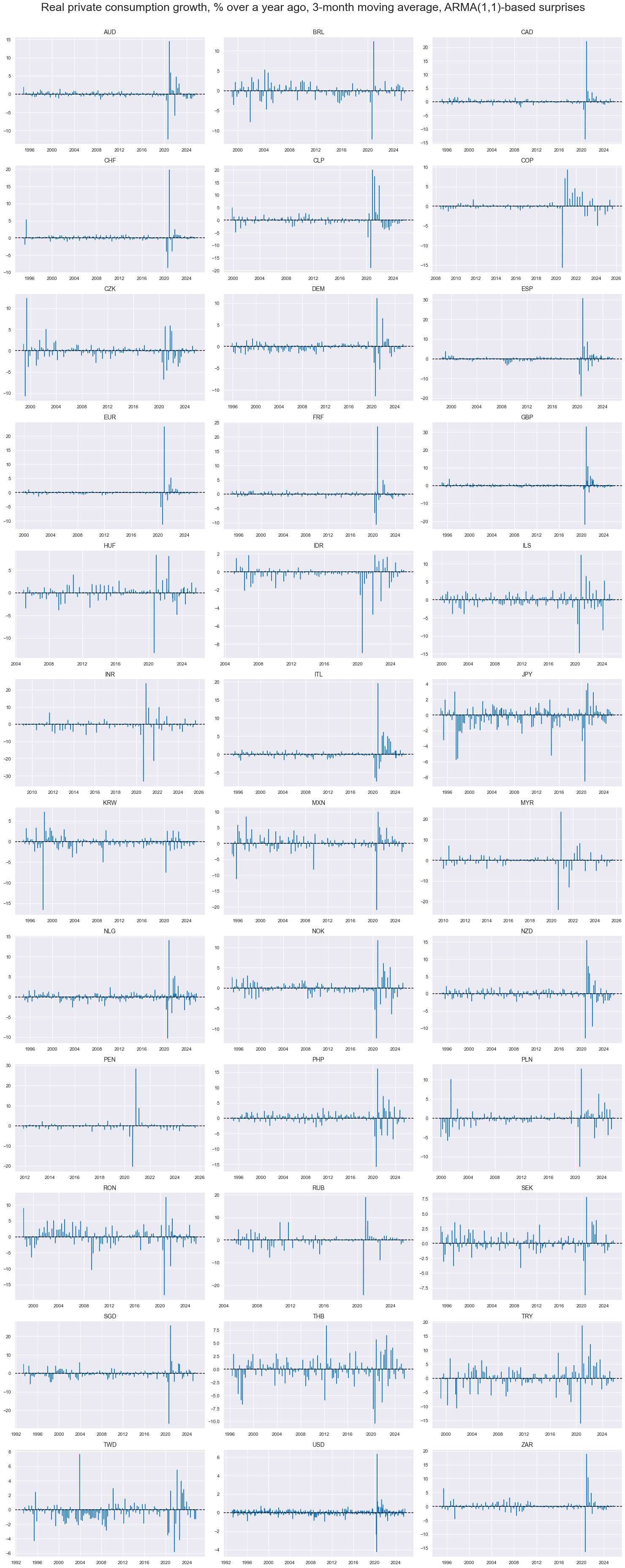
Surprises to annual private consumption trends have varied greatly across countries, partly reflecting differences in data quality. Also, the size of surprises has been very different across time, with large surprises concentrated on specific events, such as the COVID-19 pandemic.
cidx = sorted(cids_rpcons)
xcatx = ["RPCONS_SA_P1M1ML12_3MMA_ARMAS"]

msp.view_ranges(
    dfx,
    xcats=xcatx,
    cids=cidx,
    sort_cids_by="std",
    start=start_date,
    kind="bar",
    size=(16, 8),
    title="Means and standard deviations of real private consumption growth surprises since 2000",
    xcat_labels=["Real private consumption growth, % over a year ago, 3-month moving average, ARMA(1,1)-based surprises"],
)
cidx = cids_rpcons
xcatx = [
    "RPCONS_SA_P1M1ML12_3MMA_ARMAS",
]

msp.view_timelines(
    dfx,
    xcats=xcatx,
    cids=cidx,
    start=start_date,
    title="Real private consumption growth, % over a year ago, 3-month moving average, ARMA(1,1)-based surprises",
    ncol=3,
    same_y=False,
    legend_fontsize=20,
    title_fontsize=27,
    size=(12, 7),
    all_xticks=True,
    legend_ncol=2,
 )
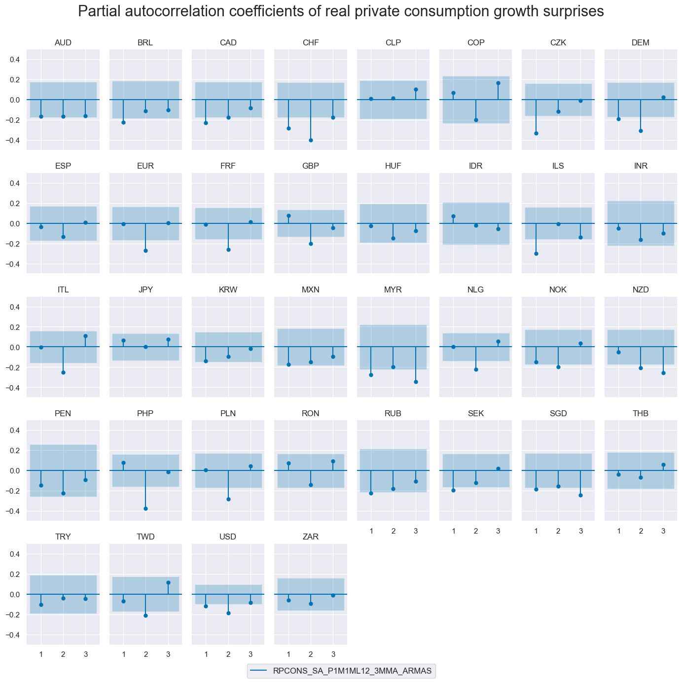
First-order autocorrelation of consumption growth surprises has mostly been negative. This suggests that surprises are often the consequence of temporary disturbances.
msv.plot_pacf(
    df=dfx,
    cids=cids,
    xcat="RPCONS_SA_P1M1ML12_3MMA_ARMAS",
    title="Partial autocorrelation coefficients of real private consumption growth surprises",
    lags=3,
    remove_zero_predictor=True,
    figsize=(14, 14),
    ncols=8,
)
Consumer confidence scores #
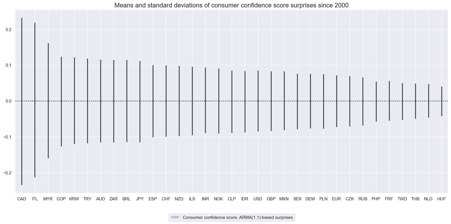
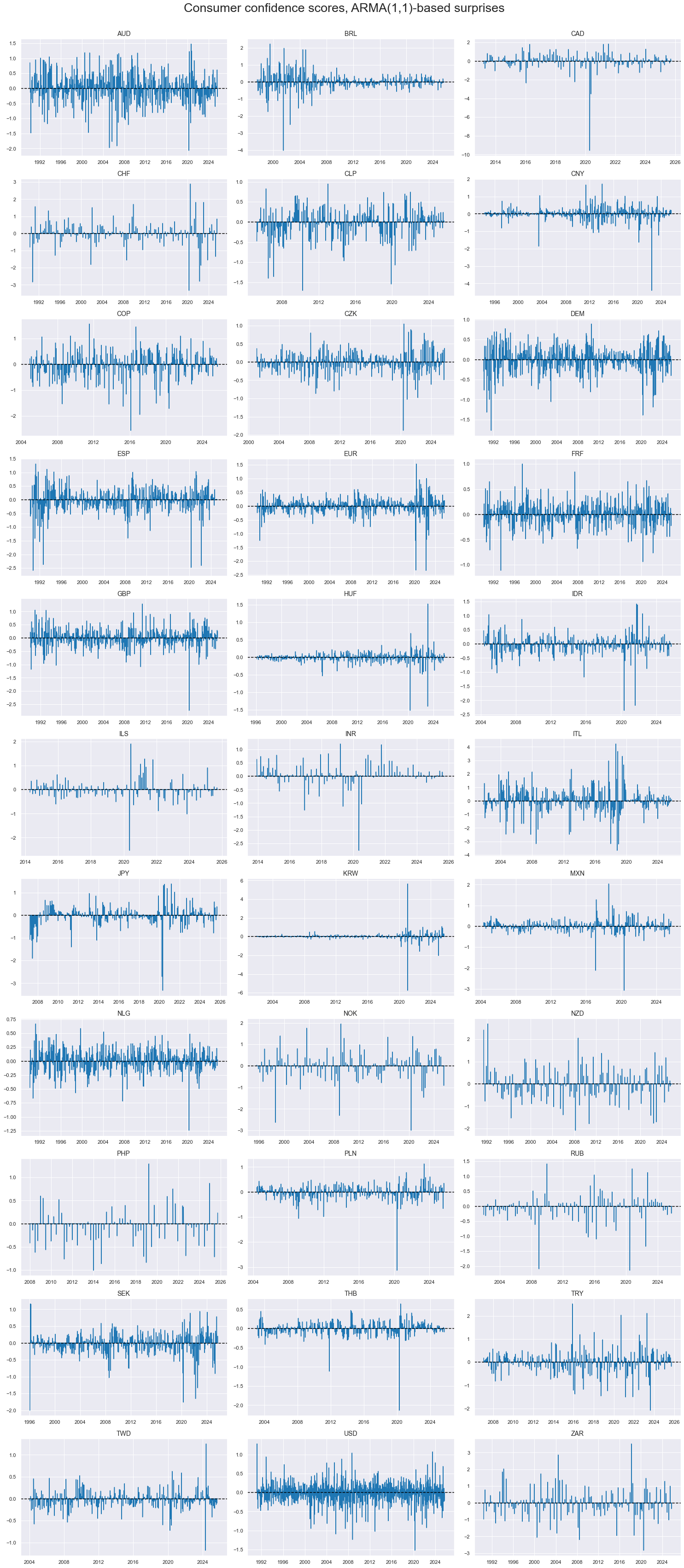
Suprises to consumer confidence scores have also varied greatly across countries. Large surprises have occurred more often in surveys than in actual private consumption growth data.
cidx = sorted(cids_rpcons)
xcatx = ["CCSCORE_SA_ARMAS"]

msp.view_ranges(
    dfx,
    xcats=xcatx,
    cids=cidx,
    sort_cids_by="std",
    start=start_date,
    kind="bar",
    size=(16, 8),
    title="Means and standard deviations of consumer confidence score surprises since 2000",
    xcat_labels=["Consumer confidence score, ARMA(1,1)-based surprises"],
)
cidx = cids_ccscore
xcatx = ["CCSCORE_SA_ARMAS"]

msp.view_timelines(
    dfx,
    xcats=xcatx,
    cids=cidx,
    start=start_date,
    title="Consumer confidence scores, ARMA(1,1)-based surprises",
    ncol=3,
    same_y=False,
    legend_fontsize=17,
    title_fontsize=27,
    size=(12, 7),
    all_xticks=True,
)
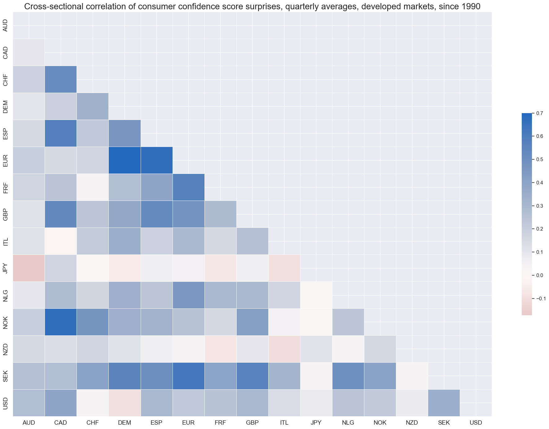
Consumer confidence surprises have not generally been positively correlated, even with the developed market groups and when averaged over quarters. This suggests that consumer confidence surveys are often driven by local factors.
cidx = cids_dm

msp.correl_matrix(
    dfx,
    xcats="CCSCORE_SA_ARMAS",
    cids=cidx,
    size=(20, 14),
    start=start_date,
    title="Cross-sectional correlation of consumer confidence score surprises, quarterly averages, developed markets, since 1990",
    title_fontsize=20,
    freq="q",
)
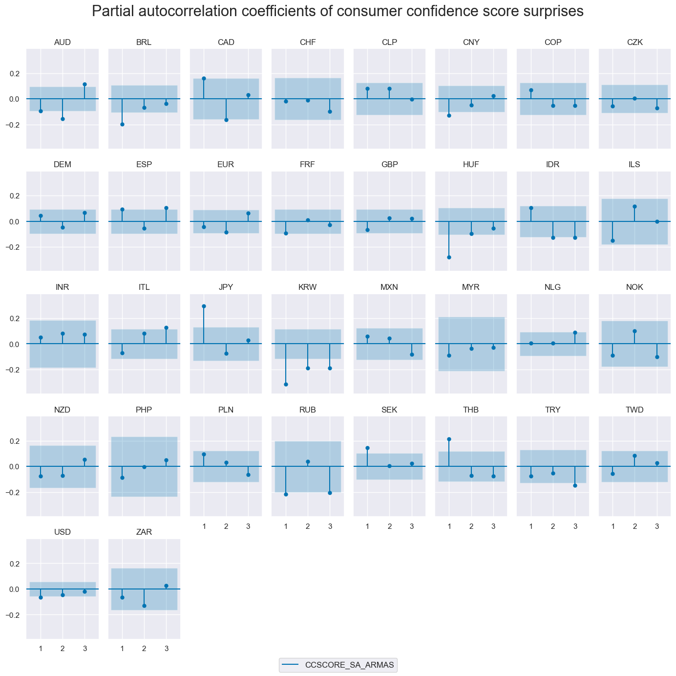
Autocorrelation of susprises has mostly need insignificant and both positive and negative across countries.
msv.plot_pacf(
    df=dfx,
    cids=cids,
    xcat="CCSCORE_SA_ARMAS",
    title="Partial autocorrelation coefficients of consumer confidence score surprises",
    lags=3,
    remove_zero_predictor=True,
    figsize=(14, 14),
    ncols=8,
)
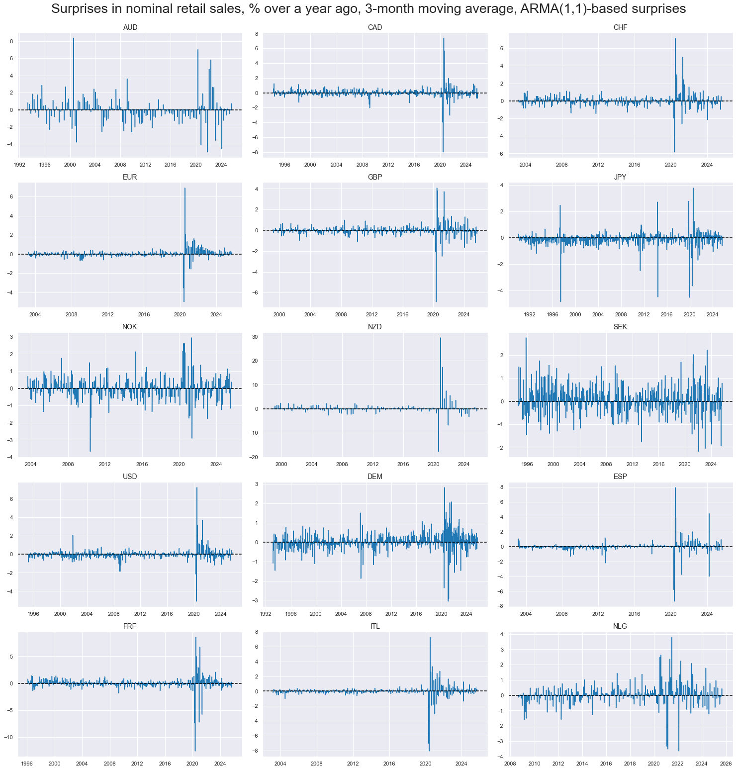
Retail sales growth #
Large surprises to retail sales growth have been concentrated on specific episodes, particularly the COVID-19 pandemic.
cidx = cids
cidx = cids_dm
xcatx = [
    "NRSALES_SA_P1M1ML12_3MMA_ARMAS",
]

msp.view_timelines(
    dfx,
    xcats=xcatx,
    cids=cidx,
    start=start_date,
    title="Surprises in nominal retail sales, % over a year ago, 3-month moving average, ARMA(1,1)-based surprises",
    ncol=3,
    same_y=False,
    legend_fontsize=17,
    title_fontsize=27,
    size=(12, 7),
    all_xticks=True,
    legend_ncol=2,
)
Importance #
Research links #
“The interaction between the macroeconomy and asset markets is central to a variety of modern theories of the business cycle. Much recent work emphasizes the joint nature of the consumption decision and the portfolio allocation decision.” Mankiw and Shapiro
on consumption and stock returns
“… consumption-based predictive variable, called cyclical consumption … captures a significant fraction of variation in expected stock returns” Atanasov, Vinther Moeller and Priestley
“… the marginal utility of consumption, when suitably modeled, can explain the trade-off between risk and return reflected in the size premium, the value premium, and the time-varying equity” M Yogo
on consumption and currency returns
“We find a strong link between currency excess returns and the relative strength of the business cycle. Buying currencies of strong economies and selling currencies of weak economies generates high returns both in the cross-section and time series of countries.” Colacito, Riddiough and Sarno
Empirical clues #
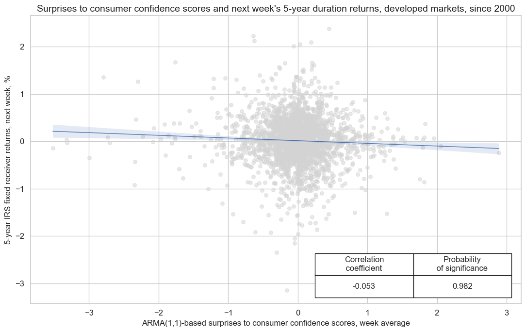
Private consumption suprises and duration returns #
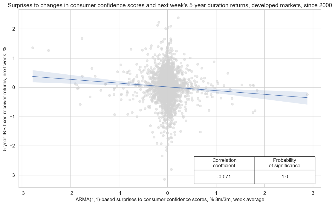
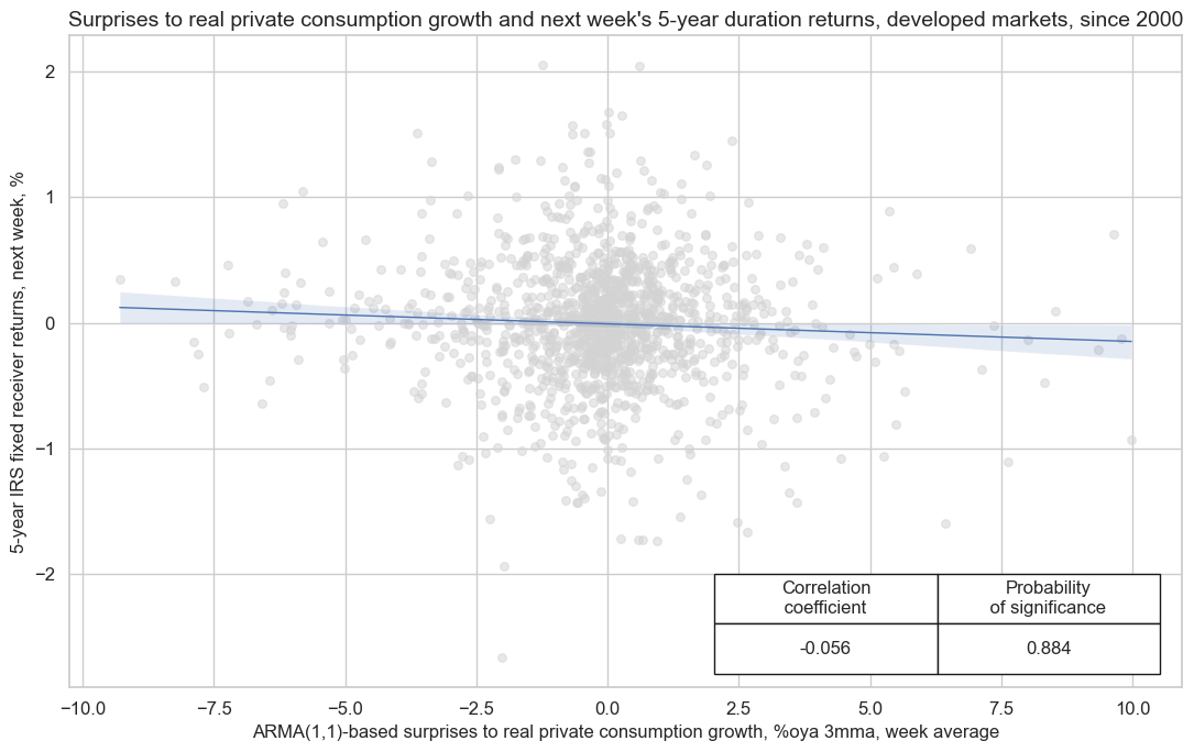
Generally stronger household sentiment and spending bodes well for economic growth and may even exert inflationary pressure. As a result, there is ample evidence of a negative relation between consumer sentiment surprises and the next week’s duration returns, as measured by 5-year fixed receiver returns for 5-year interest rate swaps contracts. There is also evidence of a negative relation between private consumption growth surprises and subsequent duration returns.
cidx = cids_dmca

cr = msp.CategoryRelations(
    dfx,
    xcats=["CCSCORE_SA_ARMAS", "DU05YXR_NSA"],  # Core CPI surprise and next-day equity returns
    cids=cidx,                                 # Developed market countries
    freq="w",
    lag=1,                                          # One-day forward relationship
    xcat_aggs=["sum", "sum"],
    fwin=1,
    start="2000-01-01",
    years=None,
    xcat_trims=[5, None]
)

cr.reg_scatter(
    coef_box="lower right",
    title="Surprises to consumer confidence scores and next week's 5-year duration returns, developed markets, since 2000",
    title_fontsize=14,
    xlab="ARMA(1,1)-based surprises to consumer confidence scores, week average",
    ylab="5-year IRS fixed receiver returns, next week, %",
    prob_est="map",
    remove_zero_predictor=True,
    size=(11, 7)
)
cidx = cids_dmca

cr = msp.CategoryRelations(
    dfx,
    xcats=["CCSCORE_SA_D3M3ML3_ARMAS", "DU05YXR_NSA"],  # Core CPI surprise and next-day equity returns
    cids=cidx,                                 # Developed market countries
    freq="w",
    lag=1,                                          # One-day forward relationship
    xcat_aggs=["sum", "sum"],
    fwin=1,
    start="2000-01-01",
    years=None,
    xcat_trims=[3, None]
)

cr.reg_scatter(
    coef_box="lower right",
    title="Surprises to changes in consumer confidence scores and next week's 5-year duration returns, developed markets, since 2000",
    title_fontsize=14,
    xlab="ARMA(1,1)-based surprises to consumer confidence scores, % 3m/3m, week average",
    ylab="5-year IRS fixed receiver returns, next week, %",
    prob_est="map",
    remove_zero_predictor=True,
    size=(11, 7)
)
cidx = cids_dmca

cr = msp.CategoryRelations(
    dfx,
    xcats=["RPCONS_SA_P3M3ML3AR_ARMAS", "DU05YXR_NSA"],  # Core CPI surprise and next-day equity returns
    cids=cidx,                                 # Developed market countries
    freq="w",
    lag=1,                                          # One-day forward relationship
    xcat_aggs=["sum", "sum"],
    fwin=1,
    start="2000-01-01",
    years=None,
    xcat_trims=[10, None]
)

cr.reg_scatter(
    coef_box="lower right",
    title="Surprises to real private consumption growth and next week's 5-year duration returns, developed markets, since 2000",
    title_fontsize=14,
    xlab="ARMA(1,1)-based surprises to real private consumption growth, %oya 3mma, week average",
    ylab="5-year IRS fixed receiver returns, next week, %",
    prob_est="map",
    remove_zero_predictor=True,
    size=(11, 7)
)
Appendices #
Appendix 1: Currency symbols #
The word ‘cross-section’ refers to currencies, currency areas or economic areas. In alphabetical order, these are AUD (Australian dollar), BRL (Brazilian real), CAD (Canadian dollar), CHF (Swiss franc), CLP (Chilean peso), CNY (Chinese yuan renminbi), COP (Colombian peso), CZK (Czech Republic koruna), DEM (German mark), ESP (Spanish peseta), EUR (Euro), FRF (French franc), GBP (British pound), HKD (Hong Kong dollar), HUF (Hungarian forint), IDR (Indonesian rupiah), ITL (Italian lira), JPY (Japanese yen), KRW (Korean won), MXN (Mexican peso), MYR (Malaysian ringgit), NLG (Dutch guilder), NOK (Norwegian krone), NZD (New Zealand dollar), PEN (Peruvian sol), PHP (Phillipine peso), PLN (Polish zloty), RON (Romanian leu), RUB (Russian ruble), SEK (Swedish krona), SGD (Singaporean dollar), THB (Thai baht), TRY (Turkish lira), TWD (Taiwanese dollar), USD (U.S. dollar), ZAR (South African rand).
Appendix 2: Quantamental economic surprises #
Quantamental economic surprises are defined as deviations of point-in-time quantamental indicators from expected values. Expected values are estimated predictions of an informed market participant. Following this definition there are two types of surprises that jointly make up economic surprise indicators:
• A first print event is the difference between a quantamental indicator on a release date and its expected value. A release date is the day on which any underlying economic time series adds an observation period. Expected values are estimated, typically based on econometric models and information prior to the release date. A quantamental data surprise is always specific to the prediction model or statistical learning process.
• A pure revision event is the change in a quantamental indicator on a non-release date. It arises from revisions of data for previously released observation periods. Per default, it is assumed that all revisions are surprises, i.e., that the latest reported value for an observation period is the best predictor its value after revisions. Note that any revisions published on a release date become part of the first print event.
A quantamental indicator of economic surprises records the values of these two events on the dates they become known. It records zero values for all other dates. Models for predicting indicator values always use the latest vintage of the underlying data series. They are typically applied to increments, i.e., differences or log differences of volume, value or price indices. The predicted next increment produces an expected new vintage, and the expected new vintage implies a new derived expected quantamental indicator, such as an annual growth rate or moving average. Note than in this way predictions automatically account for “base effects”, i.e., predictable changes in growth rates that arise from unusually sharp increase of declines in index levels of the base period, for example a year ago.
Appendix 3: Advanced-release and first-print surprises #
Consumer confidence score calculation
The USD CCSCORE series, \(CC_t\) , combines two standardized surveys:
-
\(X_t\) : University of Michigan Consumer Sentiment Index (earlier release)
-
\(Y_t\) : Conference Board Consumer Confidence Index (later release)
Given that the University of Michigan Consumer Sentiment Index is released earlier than the Conference Board Consumer Confidence Index, the calculation of the combined consumer confidence score, \(CC_t\) , involves two cases.
Case 1 (both available):
Case 2 (only \(X_t\) available):
We impute \(Y_t\) by carrying forward its last value and adding the observed changed in \(X_t\) :
University of Michigan-release surprise (First Release)
Ahead of a new early release, both \(X_{t-1}\) and \(Y_{t-1}\) are known. We can forecast \(X_{t}\) and \(Y_{t}\) (e.g. with separate ARMA models) and average them:
with the surprise calculated when the University of Michigan Consumer Sentiment Index is released.
Conference Board-release surprise (Second Release)
Once we have the early release, we impute \(\tilde Y_t\) as above, and the surprise is the revision when \(Y_t\) is released:
where \(\widetilde {CC}_{t}\) is again our estimate with the imputed \(\tilde Y_t\) .