Inflation survey indicators #
This category group features point-in-time survey scores related to inflation expectations, typically for the for the upcoming twelve months. At present it contains only household surveys.
Household inflation expectations scores #
Ticker : HHINFESCORE_NSA
Label : Household CPI inflation expectations, 1-year ahead, z-score.
Definition : Household CPI inflation expectations, 1-year ahead, z-score.
Notes :
-
Household inflation expectations are collected through surveys as expectations of CPI growth for the next 12 months. Countries publish this information as a percentage or as a diffusion index.
-
Both methodologies are made compatible through the calculation of scores based on past expanding data samples in order to replicate the market’s information state on survey readings. For in-depth explanation of how the z-scores are computed, please read Appendix 2 .
-
JPY does not publish a consolidated index, thus a diffusion index is created using the published distribution of household expectations. The formula combines all the percentages using the following weights: (-1) for expectations of inflation lower than -2%, (-0.5) for inflation between -2% and 0%, (0) for stable prices, (+0.5) for inflation between 0% and 2%, and (+1) for inflation greater than 2%.
-
All survey indices used for this metric are summarized in Appendix 3 .
Changes in household inflation expectations #
Ticker : HHINFESCORE_NSA_D1M1ML1 / _D1Q1QL1 / _D3M3ML3
Label : Change in household inflation expectation score: diff m/m / diff q/q / diff 3m/3m
Definition : Change in household inflation expectation score: latest month over one month ago / latest quarter over one quarter ago / latest three months over the previous three months.
Notes :
-
This quantamental indicator measures the difference between the expectations of the latest period versus previous period according to the concurrent data vintage. For instance, a score that goes from 0.8 to 0.9 between periods will show an increase of 0.1.
-
Currency areas with monthly frequency surveys print monthly changes (_D1M1ML1 and _D3M3ML3), and areas with quarterly frequency provide only quarterly changes (_D1Q1QL1).
Imports #
Only the standard Python data science packages and the specialized
macrosynergy
package are needed.
import os
import numpy as np
import pandas as pd
import matplotlib.pyplot as plt
import seaborn as sns
import math

import json
import yaml

import macrosynergy.management as msm
import macrosynergy.panel as msp
import macrosynergy.signal as mss
import macrosynergy.pnl as msn


from macrosynergy.download import JPMaQSDownload

from timeit import default_timer as timer
from datetime import timedelta, date, datetime

import warnings

warnings.simplefilter("ignore")
The
JPMaQS
indicators we consider are downloaded using the J.P. Morgan Dataquery API interface within the
macrosynergy
package. This is done by specifying
ticker strings
, formed by appending an indicator category code
<category>
to a currency area code
<cross_section>
. These constitute the main part of a full quantamental indicator ticker, taking the form
DB(JPMAQS,<cross_section>_<category>,<info>)
, where
<info>
denotes the time series of information for the given cross-section and category.
The following types of information are available:
-
valuegiving the latest available values for the indicator -
eop_lagreferring to days elapsed since the end of the observation period -
mop_lagreferring to the number of days elapsed since the mean observation period -
gradedenoting a grade of the observation, giving a metric of real time information quality.
After instantiating the
JPMaQSDownload
class within the
macrosynergy.download
module, one can use the
            download(tickers,


            start_date,


            metrics)
method to obtain the data. Here
tickers
is an array of ticker strings,
start_date
is the first release date to be considered and
metrics
denotes the types of information requested.
# Cross-sections of interest

cids_dmca = [
    "AUD",
    "CAD",
    "DEM",
    "ITL",
    "FRF",
    "ESP",
    "NLG",
    "EUR",
    "GBP",
    "JPY",
    "NOK",
    "NZD",
    "SEK",
    "USD"
]  # DM currency areas
cids_latm = ["BRL"]  # Latam countries
cids_emea = ["RUB", "CZK", "HUF", "PLN"]  # EMEA countries
cids_emas = [
    "INR",
    "KRW",
]  # EM Asia countries

cids_dm = cids_dmca
cids_em = cids_latm + cids_emea + cids_emas

cids = sorted(cids_dm + cids_em)
# Quantamental categories of interest

main = ["HHINFESCORE_NSA", "HHINFESCORE_NSA_D1M1ML1", "HHINFESCORE_NSA_D3M3ML3", "HHINFESCORE_NSA_D1Q1QL1"]  # main macro

econ = ["RIR_NSA"]  # economic context
mark = ["EQXR_NSA",
        "EQXR_VT10",
        "DU02YXR_VT10",
        "DU02YXR_NSA",
        "DU05YXR_VT10",
        "DU05YXR_NSA",
        "FXXR_VT10",
        "FXXR_NSA",
        ]  # market links

xcats = main + econ + mark
# Download series from J.P. Morgan DataQuery by tickers

start_date = "1990-01-01"
tickers = [cid + "_" + xcat for cid in cids for xcat in xcats]
print(f"Maximum number of tickers is {len(tickers)}")

# Retrieve credentials

client_id: str = os.getenv("DQ_CLIENT_ID")
client_secret: str = os.getenv("DQ_CLIENT_SECRET")

# Download from DataQuery

with JPMaQSDownload(client_id=client_id, client_secret=client_secret) as downloader:
    start = timer()
    df = downloader.download(
        tickers=tickers,
        start_date=start_date,
        metrics=["value", "eop_lag", "mop_lag", "grading"],
        suppress_warning=True,
    )
    end = timer()

dfd = df

print("Download time from DQ: " + str(timedelta(seconds=end - start)))
Maximum number of tickers is 273
Downloading data from JPMaQS.
Timestamp UTC:  2025-05-06 08:54:09
Connection successful!
Some expressions are missing from the downloaded data. Check logger output for complete list.
260 out of 1092 expressions are missing. To download the catalogue of all available expressions and filter the unavailable expressions, set `get_catalogue=True` in the call to `JPMaQSDownload.download()`.
Some dates are missing from the downloaded data.
2 out of 9224 dates are missing.
Download time from DQ: 0:02:45.749822
Availability #
cids_exp = sorted(
    list(set(cids))
)  # cids expected in category panels
msm.missing_in_df(dfd, xcats=main, cids=cids_exp)
No missing XCATs across DataFrame.
Missing cids for HHINFESCORE_NSA:          []
Missing cids for HHINFESCORE_NSA_D1M1ML1:  ['CAD', 'GBP', 'NOK', 'NZD', 'SEK']
Missing cids for HHINFESCORE_NSA_D1Q1QL1:  ['AUD', 'BRL', 'CZK', 'DEM', 'ESP', 'EUR', 'FRF', 'HUF', 'INR', 'ITL', 'JPY', 'KRW', 'NLG', 'PLN', 'RUB', 'USD']
Missing cids for HHINFESCORE_NSA_D3M3ML3:  ['CAD', 'GBP', 'NOK', 'NZD', 'SEK']
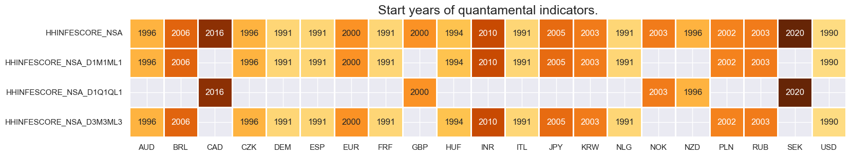
Consumer inflation expectations are available from the early 2000s for the vast majority of countries. Currency areas providing monthly data will not display quarterly changes (_D1Q1QL1) and vice-versa.
For the explanation of currency symbols, which are related to currency areas or countries for which categories are available, please view Appendix 1 .
xcatx = main
cidx = cids_exp

dfx = msm.reduce_df(dfd, xcats=xcatx, cids=cidx)
dfs = msm.check_startyears(dfx)
msm.visual_paneldates(dfs, size=(18, 3))

print("Last updated:", date.today())
Last updated: 2025-05-06
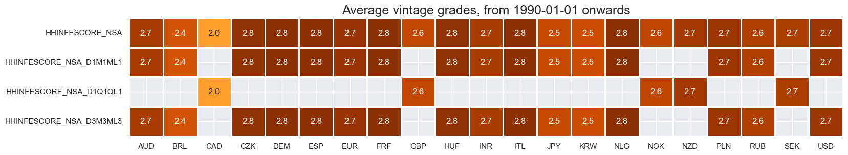
Average grades are on the low side at the moment, as electronic vintage records are not yet easily available. This, in turn, reflects that these surveys are not as carefully watched by markets.
xcatx = main
cidx = cids_exp

plot = msp.heatmap_grades(
    dfd,
    xcats=xcatx,
    cids=cidx,
    start=start_date,
    size=(18, 3),
    title=f"Average vintage grades, from {start_date} onwards",
)
History #
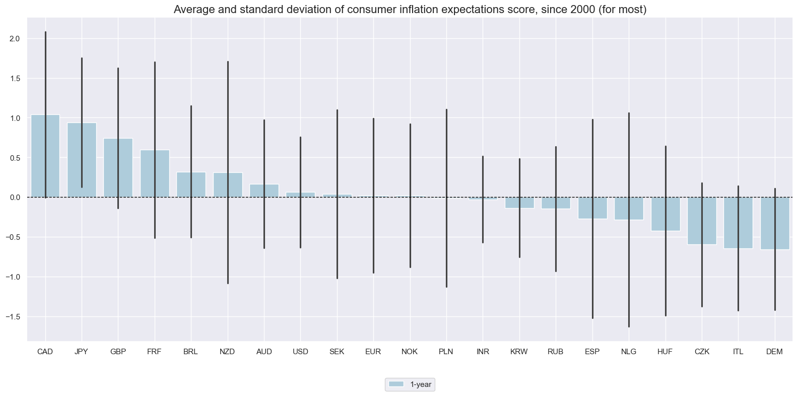
Consumer expectation of 1-year ahead inflation #
Due to (point-in-time) normalization the variation of expectation scores has been of comparable magnitude across countries. Most long-term averages are near zero, but for countries with secular inflation trends or short histories, the average can be larger than half a standard deviation.
xcatx = ["HHINFESCORE_NSA"]
cidx = cids_exp
start_date = "2000-01-01"

msp.view_ranges(
    dfd,
    xcats=xcatx,
    cids=cidx,
    sort_cids_by="mean",
    start=start_date,
    kind="bar",
    size=(16, 8),
    title="Average and standard deviation of consumer inflation expectations score, since 2000 (for most)",
    xcat_labels=["1-year"],
)
xcatx = ["HHINFESCORE_NSA"]
cidx = cids_exp
start_date = "1990-01-01"

msp.view_timelines(
    dfd,
    xcats=xcatx,
    cids=cidx,
    start=start_date,
    title="Consumer inflation expectations scores, since inception",
    legend_fontsize=17,
    label_adj=0.075,
    xcat_labels=["1-year ahead"],
    ncol=4,
    same_y=True,
    size=(12, 7),
    aspect=1.7,
    all_xticks=True,
)
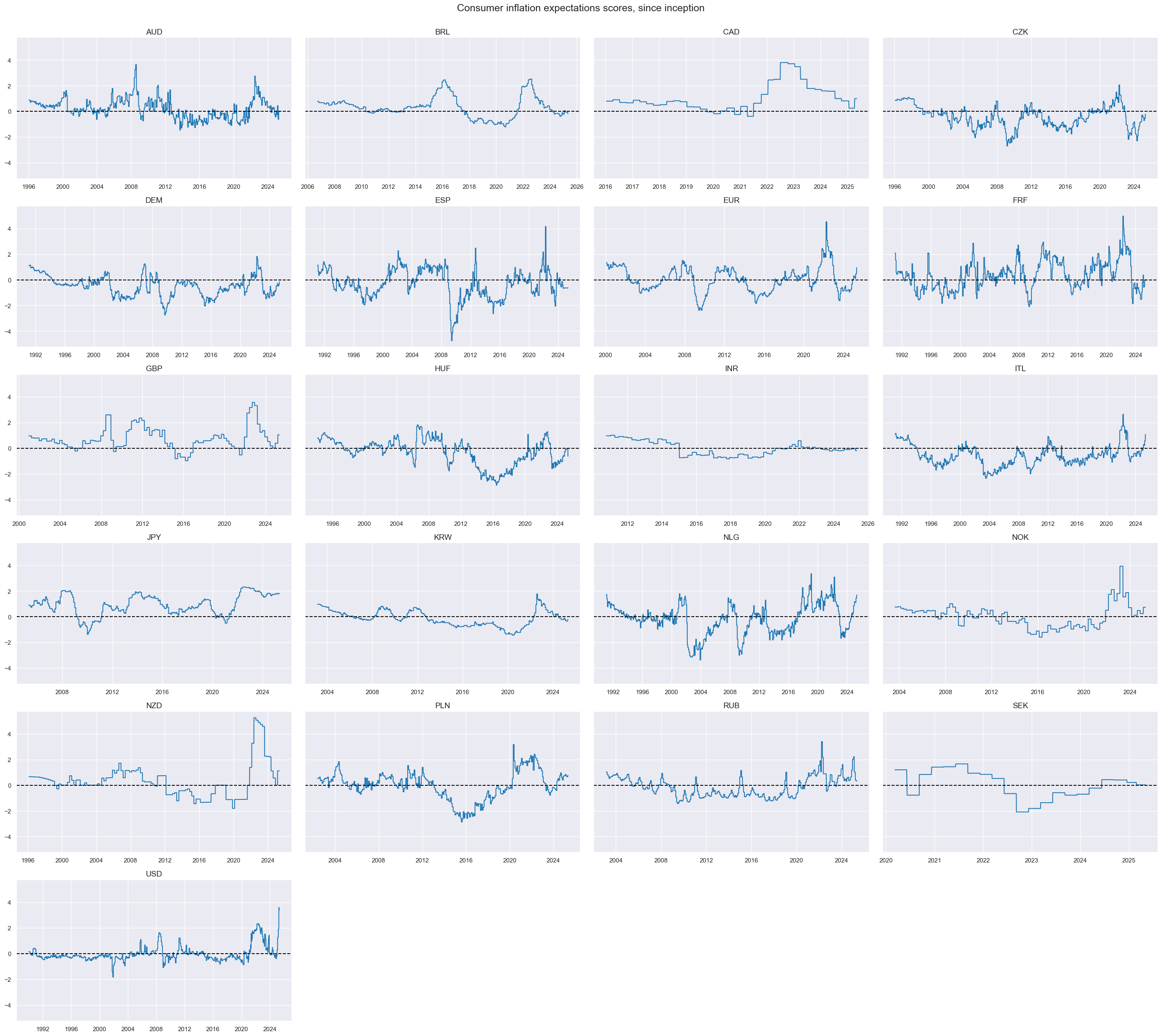
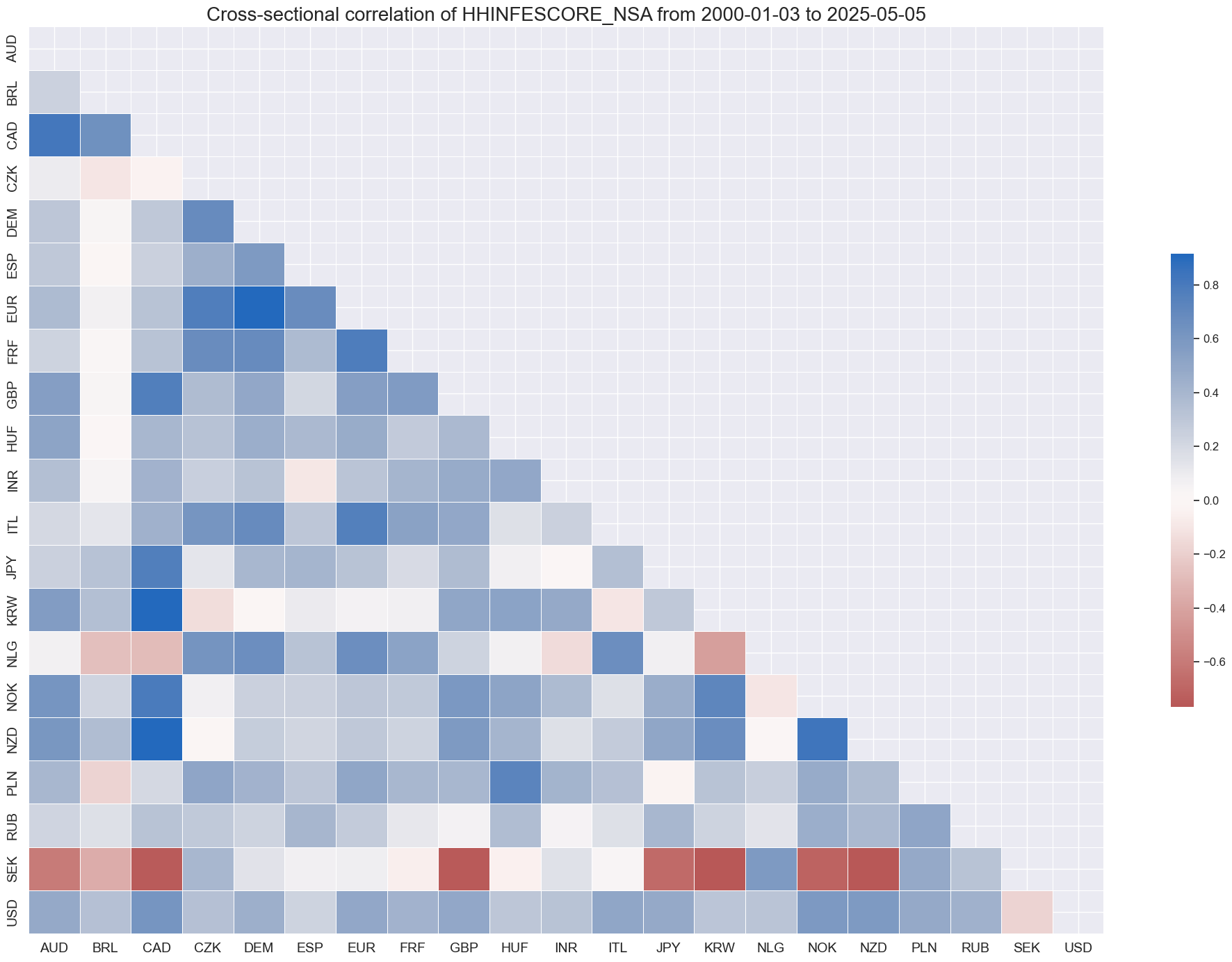
Consumer inflation expectations have been mostly positively correlated across countries. Sweden has been an exceptions, but that may largely reflect its short history.
xcatx = "HHINFESCORE_NSA"
cidx = cids_exp

msp.correl_matrix(dfd, xcats=xcatx, cids=cidx, size=(20, 14))
Importance #
Research links #
“Inflation expectations wield great influence over fixed income returns. They determine the nominal yield required for a given equilibrium real interest rate, they influence inflation risk premia, and they shape the central bank’s course of action. There is no uniform inflation expectation metric than can be tracked in real-time. However, there are useful and complementary proxies, such as market-based breakeven inflation and economic data-based estimates. For trading strategies, these two can be combined. The advantage of breakeven rates is the real-time tracking of a broad range of influences. The advantages of economic data-based estimates are clarity, transparency, and precision of measurement. Changes in both inflation metrics help predict interest rate swap returns, but their combination is a better predictor than the individual series, emphasizing the complementarity of market and economic data.” Macrosynergy
“A theoretical paper shows that a downward shift in expected inflation increases equity valuations and credit default risk at the same time. The reason for this is ‘nominal stickiness’. A slowdown in consumer prices reduces short-term interest rates but does not immediately reduce earnings growth by the same rate, thus increasing the discounted present value of future earnings. At the same time, a downward shift in expected inflation increases future real debt service and leverage of firms and increases their probability of default. This theory is supported by the trends in U.S. markets since 1970.” Macrosynergy
“Two recent empirical studies highlight the risk that inflation expectations in the euro area are becoming de-anchored, similar to Japan. De-anchoring means that short-term price shocks can change long-term expectations. Importantly, the papers suggest medium- and short-term measures to track this de-anchoring. De-anchoring increases the risk of actual deflation and may add to the risk premia on equity and credit.” Macrosynergy
Empirical clues #
dfx = dfd.copy()

dict_repl = {
    "HHINFESCORE_NSA_D1Q1QL1": "HHINFESCORE_NSA_D3M3ML3",
}
for key, value in dict_repl.items():
    dfx["xcat"] = dfx["xcat"].str.replace(key, value)
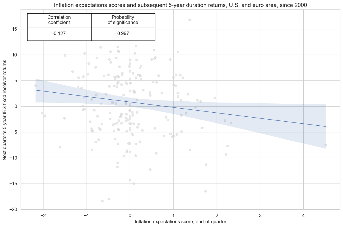
There has been a clear and significant negative relation between inflation expectation scores and subsequent vol-targeted duration returns in the U.S. and the euro area, at both the monthly and quarterly frequency.
xcatx = ["HHINFESCORE_NSA", "DU05YXR_VT10"]
cidx = ["EUR", "USD"]
start_date = "2000-01-01"

cr = msp.CategoryRelations(
    dfx,
    xcats=xcatx,
    cids=cidx,
    freq="Q",
    lag=1,
    xcat_aggs=["last", "sum"],
    start=start_date,
    years=None,
)

cr.reg_scatter(
    title="Inflation expectations scores and subsequent 5-year duration returns, U.S. and euro area, since 2000",
    labels=False,
    reg_order=1,
    coef_box="upper left",
    xlab="Inflation expectations score, end-of-quarter",
    ylab="Next quarter's 5-year IRS fixed receiver returns",
    reg_robust=True,
    prob_est='map',
)
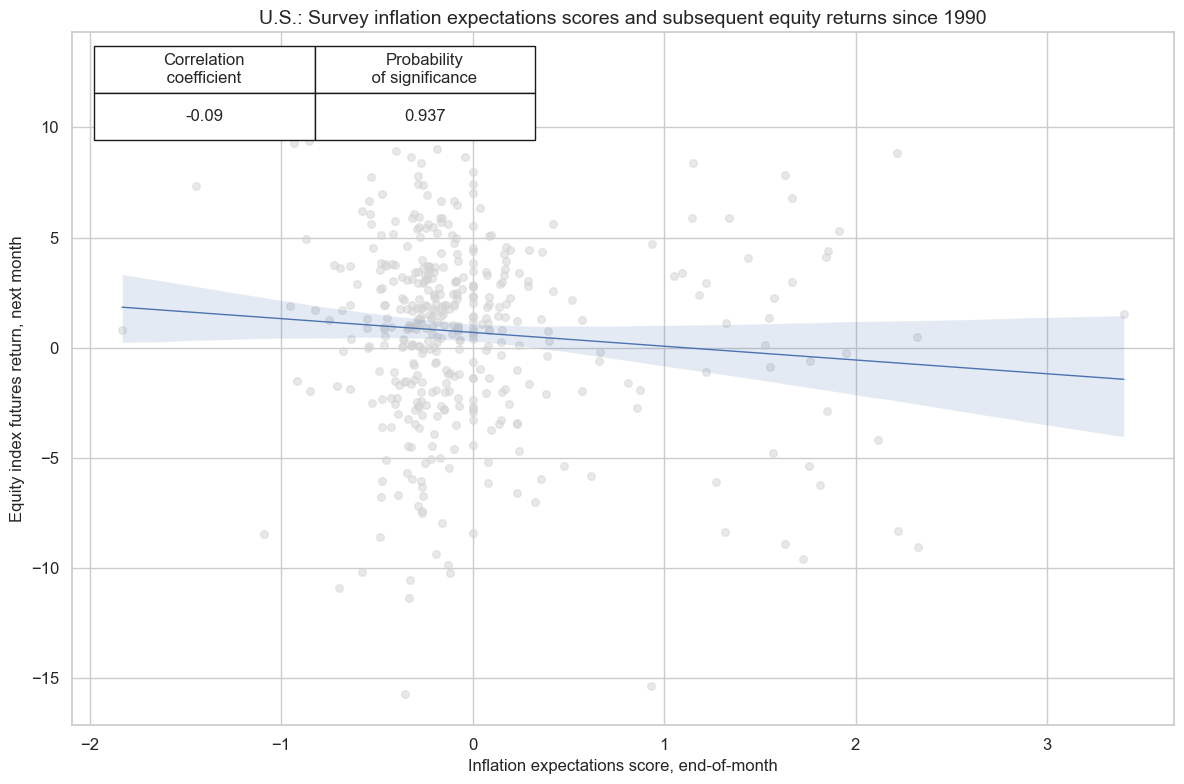
There is some evidence of a negative relationship between inflation expectation scores and subsequent equity returns in the U.S., at the monthly and quarterly frequency.
xcatx = ["HHINFESCORE_NSA", "EQXR_NSA"]
cidx = ["USD"]
start_date = "1990-01-01"

cr = msp.CategoryRelations(
    dfx,
    xcats=xcatx,
    cids=cidx,
    freq="M",
    lag=1,
    xcat_aggs=["last", "sum"],
    start=start_date,
    years=None,
)

cr.reg_scatter(
    title="U.S.: Survey inflation expectations scores and subsequent equity returns since 1990",
    labels=False,
    reg_order=1,
    coef_box="upper left",
    xlab="Inflation expectations score, end-of-month",
    ylab="Equity index futures return, next month",
)
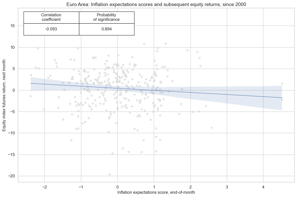
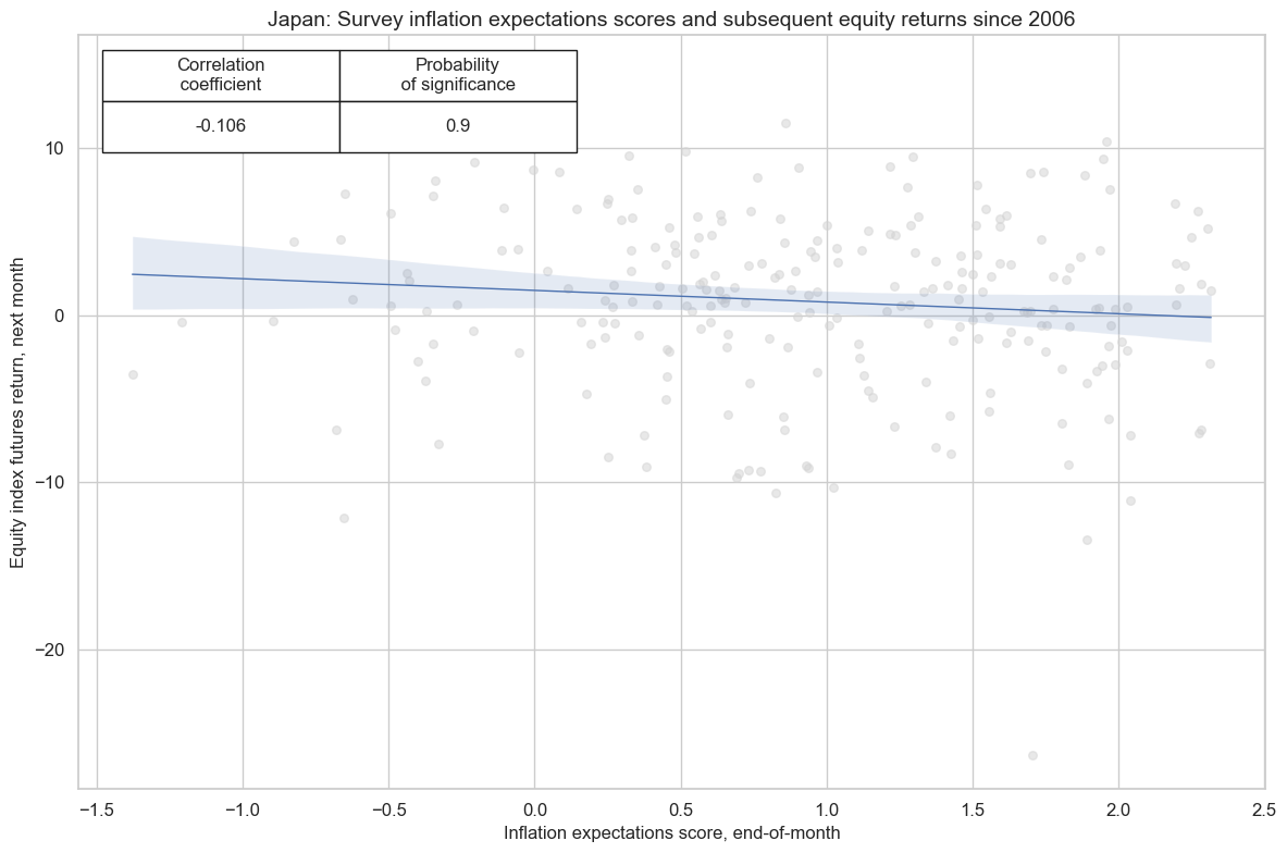
There are also signs of a negative relationship between inflation expectation scores and subsequent equity returns in the euro area and Japan, albeit not quite statistically significant. While inflation surveys are valid indicators at the country level, they are less suitable for cross-country predictions as they have different interpretations.
xcatx = ["HHINFESCORE_NSA", "EQXR_NSA"]
cidx = ['EUR']
start_date = "1999-01-01"

cr = msp.CategoryRelations(
    dfx,
    xcats=xcatx,
    cids=cidx,
    freq="M",
    lag=1,
    xcat_aggs=["last", "sum"],
    start=start_date,
    years=None,
)

cr.reg_scatter(
    title="Euro Area: Inflation expectations scores and subsequent equity returns, since 2000",
    labels=False,
    reg_order=1,
    coef_box="upper left",
    xlab="Inflation expectations score, end-of-month",
    ylab="Equity index futures return, next month",
)
xcatx = ["HHINFESCORE_NSA", "EQXR_NSA"]
cidx = ['JPY']
start_date = "1990-01-01"

cr = msp.CategoryRelations(
    dfx,
    xcats=xcatx,
    cids=cidx,
    freq="M",
    lag=1,
    xcat_aggs=["last", "sum"],
    start=start_date,
    years=None,
)

cr.reg_scatter(
    title="Japan: Survey inflation expectations scores and subsequent equity returns since 2006",
    labels=False,
    reg_order=1,
    coef_box="upper left",
    xlab="Inflation expectations score, end-of-month",
    ylab="Equity index futures return, next month",
)
Appendices #
Appendix 1: Currency symbols #
The word ‘cross-section’ refers to currencies, currency areas or economic areas. In alphabetical order, these are AUD (Australian dollar), BRL (Brazilian real), CAD (Canadian dollar), CHF (Swiss franc), CLP (Chilean peso), CNY (Chinese yuan renminbi), COP (Colombian peso), CZK (Czech Republic koruna), DEM (German mark), ESP (Spanish peseta), EUR (Euro), FRF (French franc), GBP (British pound), HKD (Hong Kong dollar), HUF (Hungarian forint), IDR (Indonesian rupiah), ITL (Italian lira), JPY (Japanese yen), KRW (Korean won), MXN (Mexican peso), MYR (Malaysian ringgit), NLG (Dutch guilder), NOK (Norwegian krone), NZD (New Zealand dollar), PEN (Peruvian sol), PHP (Phillipine peso), PLN (Polish zloty), RON (Romanian leu), RUB (Russian ruble), SEK (Swedish krona), SGD (Singaporean dollar), THB (Thai baht), TRY (Turkish lira), TWD (Taiwanese dollar), USD (U.S. dollar), ZAR (South African rand).
Appendix 2: Methodology of scoring #
The inflation expectation values are transformed into z-scores based on past expanding data samples in order to replicate the market’s information state on survey readings relative to what is considered as “normal”.
The underlying economic data used to develop the above indicators comes in the form of diffusion index or a percentage.
In order to standardise different survey indicators, we apply a custom z-scoring methodology to each survey’s vintage. We compute the mean absolute deviation to normalize deviations of confidence levels from their estimated neutral level. We require at least 12 observations to estimate it.
We finally calculate the z-score for the vintage values as
where \(X_{i, t}\) is the value of the indicator for country \(i\) at time \(t\) , \(\bar{X_i|t}\) is the measure of central tendency for country \(i\) at time \(t\) based on information up to that date, and \(\sigma_i|t\) is the mean absolute deviation for country \(i\) at time \(t\) based on information up to that date.
Appendix 3: Survey details #
surveys = pd.DataFrame(
    [
        {"country": "Australia", "source": "Melbourne Institute", "details": "Inflationary Expectations"},
        {"country": "Brazil", "source": "Getulio Vargas Foundation", "details": "Consumer Confidence Index, Inflation Expectations"},
        {"country": "Canada", "source": "Bank of Canada", "details": "Consumer Expectations, 1-Year-Ahead Inflation Expectations"},
        {"country": "Euro Area", "source": "DG ECFIN", "details": "Consumer Surveys, Price Trends Over Next 12 Months"},
        {"country": "India", "source": "Reserve Bank", "details": "Inflation Expectations Survey of Households, One Year Ahead"},
        {"country": "Japan", "source": "Cabinet Office", "details": "Consumer Confidence, Price Expectation Next 1 Year (Composite score)"},
        {"country": "New Zealand", "source": "Reserve Bank", "details": "Inflationary Expectations (1-Year)"},
        {"country": "Norway", "source": "Bank of Norway", "details": "Expectations Survey, Expected Price Change in Next 12 Months"},
        {"country": "Russia", "source": "Central Bank", "details": "Households Inflationary Expectations"},
        {"country": "South Korea", "source": "Bank of Korea", "details": "Inflationary Expectations (1 year)"},
        {"country": "Sweden", "source": "SBAB", "details": "Consumer Confidence, Price Expectation (1 Year)"},
        {"country": "United Kingdom", "source": "Bank of England", "details": "Inflation Attitudes Survey, Expected Prices in the Shops Change Over the Next 12 Months"},
        {"country": "United States", "source": "University of Michigan", "details": "Consumer Sentiment, Expected Change in Inflation Rates"},
    ]
)
from IPython.display import HTML
HTML(surveys.to_html(index=False))
| country | source | details |
|---|---|---|
| Australia | Melbourne Institute | Inflationary Expectations |
| Brazil | Getulio Vargas Foundation | Consumer Confidence Index, Inflation Expectations |
| Canada | Bank of Canada | Consumer Expectations, 1-Year-Ahead Inflation Expectations |
| Euro Area | DG ECFIN | Consumer Surveys, Price Trends Over Next 12 Months |
| India | Reserve Bank | Inflation Expectations Survey of Households, One Year Ahead |
| Japan | Cabinet Office | Consumer Confidence, Price Expectation Next 1 Year (Composite score) |
| New Zealand | Reserve Bank | Inflationary Expectations (1-Year) |
| Norway | Bank of Norway | Expectations Survey, Expected Price Change in Next 12 Months |
| Russia | Central Bank | Households Inflationary Expectations |
| South Korea | Bank of Korea | Inflationary Expectations (1 year) |
| Sweden | SBAB | Consumer Confidence, Price Expectation (1 Year) |
| United Kingdom | Bank of England | Inflation Attitudes Survey, Expected Prices in the Shops Change Over the Next 12 Months |
| United States | University of Michigan | Consumer Sentiment, Expected Change in Inflation Rates |