Industrial production trend surprises #
This category group contains economic surprise indicators related to industrial production growth trends . Economic surprises are deviations of point-in-time quantamental indicators from predicted values. For an in-depth explanation, please read Appendix 2 .
Industrial production growth surprises #
Ticker : IP_SA_P1M1ML12_3MMA_ARMAS
Label : Industrial production, % oya, 3mma, ARMA(1,1)-based surprises
Definition : Industrial production, % over year ago, 3-month moving average, ARMA(1,1)-based surprises
Notes :
-
Refer to the section on industrial production growth trends for notes on the underlying data series.
-
Expected values for release dates are based on an “ARMA(1,1)” model. This is a simple univariate time series model that predicts increments based on an autoregressive component, i.e., last period’s value, and a moving average component, represented by last period’s error. The coefficients of the model are estimated sequentially based on the vintages of production indices. And each vintage-specific model produces a one-step-ahead forecast for the subsequent observation period.
Ticker : IP_SA_P3M3ML3AR_ARMAS / _P6M6ML6AR_ARMAS / _4MMM_P1M1ML4AR_ARMAS / _P1Q1QL1AR_ARMAS / _P2Q2QL2AR_ARMAS / _P1Q1QL4_ARMAS
Label : Industrial production growth, sa, ARMA(1,1)-based surprises : % 3m/3m ar / % 6m/6m ar / % 4mm/4mm ar / % 1q/1q ar / % 2q/2q ar / % oya (q)
Definition : Industrial production surprises, seasonally and calendar adjusted, ARMA(1,1)-based surprises: % of latest 3 months over previous 3 months at an annualized rate / % of latest 6 months over previous 6 months at an annualized rate / % 4-month median over previous 4-month median at an annualized rate / % of latest quarter over previous quarter at an annualized rate / % of latest 2 quarters over previous 2 quarters at an annualized rate / % of latest quarter over quarter one year ago
Notes :
-
Refer to the section on industrial production growth trends for notes on the underlying data series.
-
Expected values for release dates are based on an “ARMA(1,1)” model. This is a simple univariate time series model that predicts increments based on an autoregressive component, i.e., last period’s value, and a moving average component, represented by last period’s error. The coefficients of the model are estimated sequentially based on the vintages of production indices. And each vintage-specific model produces a one-step-ahead forecast for the subsequent observation period.
Imports #
Only the standard Python data science packages and the specialized
macrosynergy
package are needed.
import os
import numpy as np
import pandas as pd
import matplotlib.pyplot as plt
import seaborn as sns
import math

import json
import yaml

import macrosynergy.management as msm
import macrosynergy.panel as msp
import macrosynergy.signal as mss
import macrosynergy.pnl as msn
import macrosynergy.visuals as msv

from macrosynergy.download import JPMaQSDownload

from timeit import default_timer as timer
from datetime import timedelta, date, datetime

import warnings

warnings.simplefilter("ignore")
The
JPMaQS
indicators we consider are downloaded using the J.P. Morgan Dataquery API interface within the
macrosynergy
package. This is done by specifying
ticker strings
, formed by appending an indicator category code
<category>
to a currency area code
<cross_section>
. These constitute the main part of a full quantamental indicator ticker, taking the form
DB(JPMAQS,<cross_section>_<category>,<info>)
, where
<info>
denotes the time series of information for the given cross-section and category. The following types of information are available:
-
valuegiving the latest available values for the indicator -
eop_lagreferring to days elapsed since the end of the observation period -
mop_lagreferring to the number of days elapsed since the mean observation period -
gradedenoting a grade of the observation, giving a metric of real time information quality.
After instantiating the
JPMaQSDownload
class within the
macrosynergy.download
module, one can use the
download(tickers,start_date,metrics)
method to easily download the necessary data, where
tickers
is an array of ticker strings,
start_date
is the first collection date to be considered and
metrics
is an array comprising the times series information to be downloaded.
# Cross-sections of interest

cids_dmca = [
    "AUD",
    "CAD",
    "CHF",
    "EUR",
    "GBP",
    "JPY",
    "NOK",
    "NZD",
    "SEK",
    "USD",
]  # DM currency areas
cids_dmec = ["DEM", "ESP", "FRF", "ITL", "NLG"]  # DM euro area countries
cids_latm = ["BRL", "COP", "CLP", "MXN", "PEN"]  # Latam countries
cids_emea = ["CZK", "HUF", "ILS", "PLN", "RON", "RUB", "TRY", "ZAR"]  # EMEA countries
cids_emas = [
    "CNY",
    # "HKD",
    "IDR",
    "INR",
    "KRW",
    "MYR",
    "PHP",
    "SGD",
    "THB",
    "TWD",
]  # EM Asia countries

cids_dm = cids_dmca + cids_dmec
cids_em = cids_latm + cids_emea + cids_emas

cids = sorted(cids_dm + cids_em)
# Quantamental categories of interest

main = [
    # Indicators and Forecast and Revision Surprises
    f"IP_SA_{transform}{model}"
    for transform in ("P3M3ML3AR", "P6M6ML6AR", "P1M1ML12_3MMA", "4MMM_P1M1ML4AR")
    for model in ["_ARMAS",]
] + [
      # Indicators and Forecast and Revision Surprises
    f"IP_SA_{transform}{model}"
    for transform in ("P1Q1QL1AR", "P2Q2QL2AR", "P1Q1QL4")
    for model in ["_ARMAS",]
]

econ = ["RIR_NSA", "IVAWGT_SA_1YMA"]  # economic context
mark = [
    "FXXR_NSA",
    "FXXR_VT10",
    "DU02YXR_NSA",
    "DU02YXR_VT10",
    "DU05YXR_NSA",
    "DU05YXR_VT10",
    "FXUNTRADABLE_NSA",
    "FXTARGETED_NSA",
]  # market links

xcats = main + econ + mark
# Special industry-related commodity data set
cids_co = ["ALM", "CPR", "LED", "NIC", "TIN", "ZNC"]
xcats_co = ["COXR_VT10", "COXR_NSA"]
tix_co = [c + "_" + x for c in cids_co for x in xcats_co]
# Download series from J.P. Morgan DataQuery by tickers

start_date = "1990-01-01"
tickers = [cid + "_" + xcat for cid in cids for xcat in xcats] + tix_co
print(f"Maximum number of tickers is {len(tickers)}")

# Retrieve credentials

client_id: str = os.getenv("DQ_CLIENT_ID")
client_secret: str = os.getenv("DQ_CLIENT_SECRET")

# Download from DataQuery
start = timer()
with JPMaQSDownload(client_id=client_id, client_secret=client_secret) as downloader:
    df = downloader.download(
        tickers=tickers,
        start_date=start_date,
        metrics=["value", "eop_lag", "mop_lag", "grading"],
        suppress_warning=True,
        show_progress=True,
    )
    end = timer()
dfd = df

print("Download time from DQ: " + str(timedelta(seconds=end - start)))
Maximum number of tickers is 641
Downloading data from JPMaQS.
Timestamp UTC:  2025-04-10 11:02:03
Connection successful!
Requesting data: 100%|██████████| 129/129 [00:26<00:00,  4.89it/s]
Downloading data: 100%|██████████| 129/129 [00:55<00:00,  2.32it/s]
Some expressions are missing from the downloaded data. Check logger output for complete list.
732 out of 2564 expressions are missing. To download the catalogue of all available expressions and filter the unavailable expressions, set `get_catalogue=True` in the call to `JPMaQSDownload.download()`.
Download time from DQ: 0:01:31.465277
Availability #
cids_exp = sorted(list(set(cids) - set(cids_dmec)))  # cids expected in category panels
msm.missing_in_df(dfd, xcats=main, cids=cids_exp)
No missing XCATs across DataFrame.
Missing cids for IP_SA_4MMM_P1M1ML4AR_ARMAS:  ['AUD', 'CHF', 'CNY', 'NZD']
Missing cids for IP_SA_P1M1ML12_3MMA_ARMAS:   ['AUD', 'CHF', 'NZD']
Missing cids for IP_SA_P1Q1QL1AR_ARMAS:       ['BRL', 'CAD', 'CLP', 'CNY', 'COP', 'CZK', 'EUR', 'GBP', 'HUF', 'IDR', 'ILS', 'INR', 'JPY', 'KRW', 'MXN', 'MYR', 'NOK', 'PEN', 'PHP', 'PLN', 'RON', 'RUB', 'SEK', 'SGD', 'THB', 'TRY', 'TWD', 'USD', 'ZAR']
Missing cids for IP_SA_P1Q1QL4_ARMAS:         ['BRL', 'CAD', 'CLP', 'CNY', 'COP', 'CZK', 'EUR', 'GBP', 'HUF', 'IDR', 'ILS', 'INR', 'JPY', 'KRW', 'MXN', 'MYR', 'NOK', 'PEN', 'PHP', 'PLN', 'RON', 'RUB', 'SEK', 'SGD', 'THB', 'TRY', 'TWD', 'USD', 'ZAR']
Missing cids for IP_SA_P2Q2QL2AR_ARMAS:       ['BRL', 'CAD', 'CLP', 'CNY', 'COP', 'CZK', 'EUR', 'GBP', 'HUF', 'IDR', 'ILS', 'INR', 'JPY', 'KRW', 'MXN', 'MYR', 'NOK', 'PEN', 'PHP', 'PLN', 'RON', 'RUB', 'SEK', 'SGD', 'THB', 'TRY', 'TWD', 'USD', 'ZAR']
Missing cids for IP_SA_P3M3ML3AR_ARMAS:       ['AUD', 'CHF', 'CNY', 'NZD']
Missing cids for IP_SA_P6M6ML6AR_ARMAS:       ['AUD', 'CHF', 'CNY', 'NZD']
cidx = cids_exp
xcatx = main
msm.check_availability(
    df=dfd,
    xcats=xcatx,
    cids=cidx,
    missing_recent=False,
)
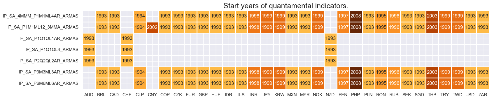
Most real-time quantamental indicators of industrial production trends are available from the early 1990s. Indeed, this is true for all developed markets and most emerging markets. Malaysia, the Phillipines and Thailand are notable late starters, with data only available post-2000.
For the explanation of currency symbols, which are related to currency areas or countries for which categories are available, please view Appendix 1 .
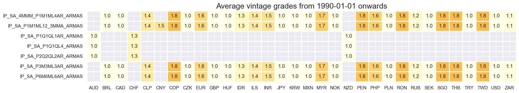
Vintage grading is perfect for most developed markets and some emerging economies.
xcatx = main
cidx = cids_exp

plot = msp.heatmap_grades(
    dfd,
    xcats=xcatx,
    cids=cidx,
    size=(18, 3),
    title=f"Average vintage grades from {start_date} onwards",
)
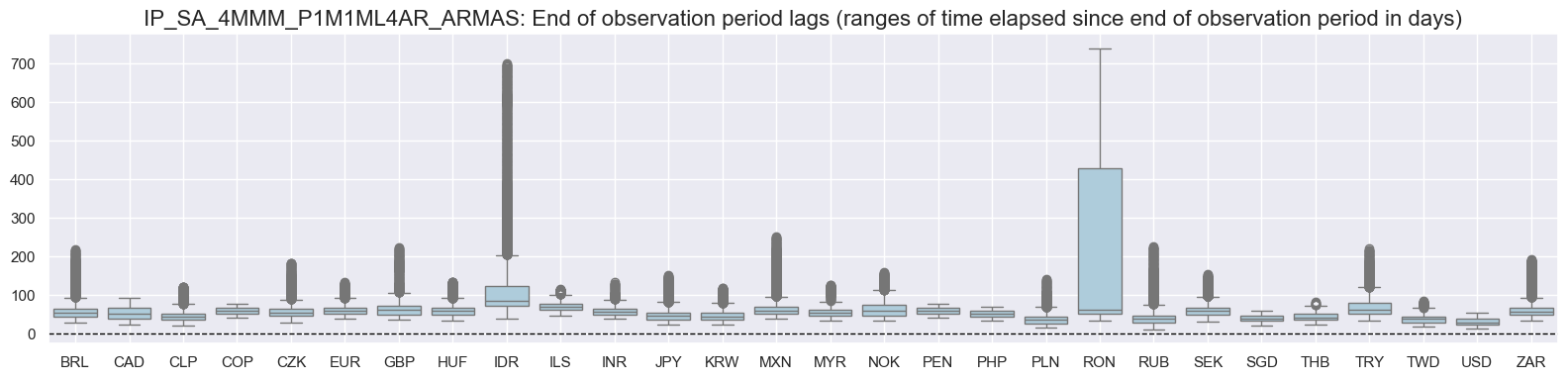
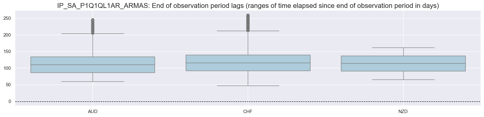
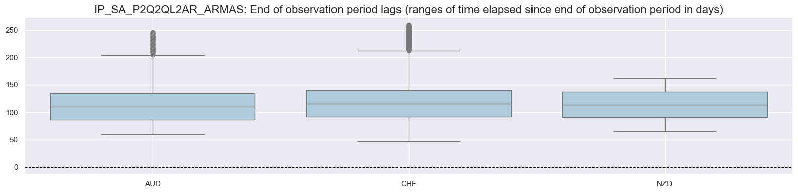
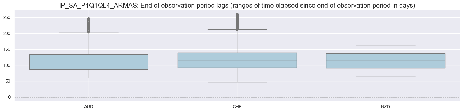
cidx = cids_exp
xcats = [xc for xc in main if xc.split("_")[-1] in ("ARMAS")]
for x in xcats:
if x not in dfd.xcat.unique():
print("No values found in data-frame for:", x)
continue
xcatx = [x]
msp.view_ranges(
dfd,
xcats=xcatx,
cids=cidx,
val="eop_lag",
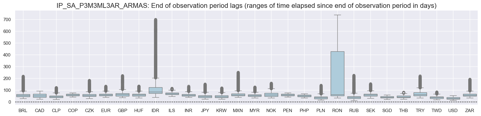
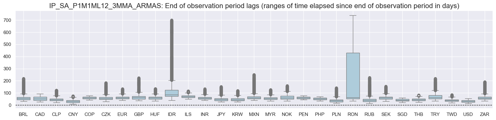
title=f"{x:s}: End of observation period lags (ranges of time elapsed since end of observation period in days)",
start=start_date,
kind="box",
size=(16, 4),
)

dict_repl = {
    # Industrial Product trends: Forecasts and Revision Surprises
    "IP_SA_P1Q1QL1AR_ARMAS": "IP_SA_P3M3ML3AR_ARMAS",
    "IP_SA_P2Q2QL2AR_ARMAS": "IP_SA_P6M6ML6AR_ARMAS",
    "IP_SA_P1Q1QL4_ARMAS": "IP_SA_P1M1ML12_3MMA_ARMAS",
}

for key, value in dict_repl.items():
    dfd["xcat"] = dfd["xcat"].str.replace(key, value)
History #
Industrial production growth surprises #
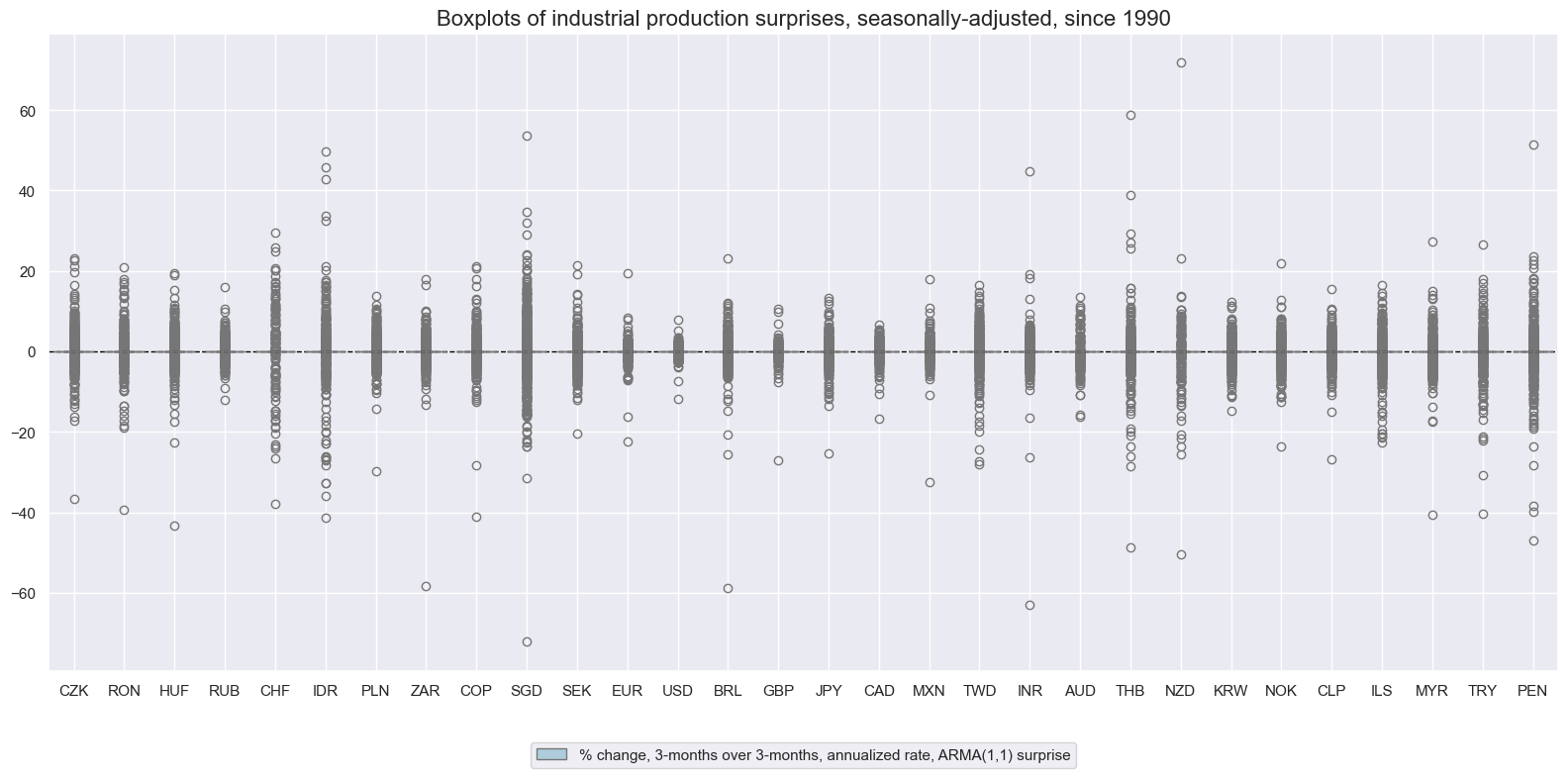
xcatx = ["IP_SA_P3M3ML3AR_ARMAS"]
cidx = list(set(cids_exp) - set(["PHP"]))


msp.view_ranges(
    dfd,
    xcats=xcatx,
    cids=cidx,
    sort_cids_by="mean",
    start=start_date,
    kind="box",
    title="Boxplots of industrial production surprises, seasonally-adjusted, since 1990",
    xcat_labels=["% change, 3-months over 3-months, annualized rate, ARMA(1,1) surprise",],
    size=(16, 8),
)
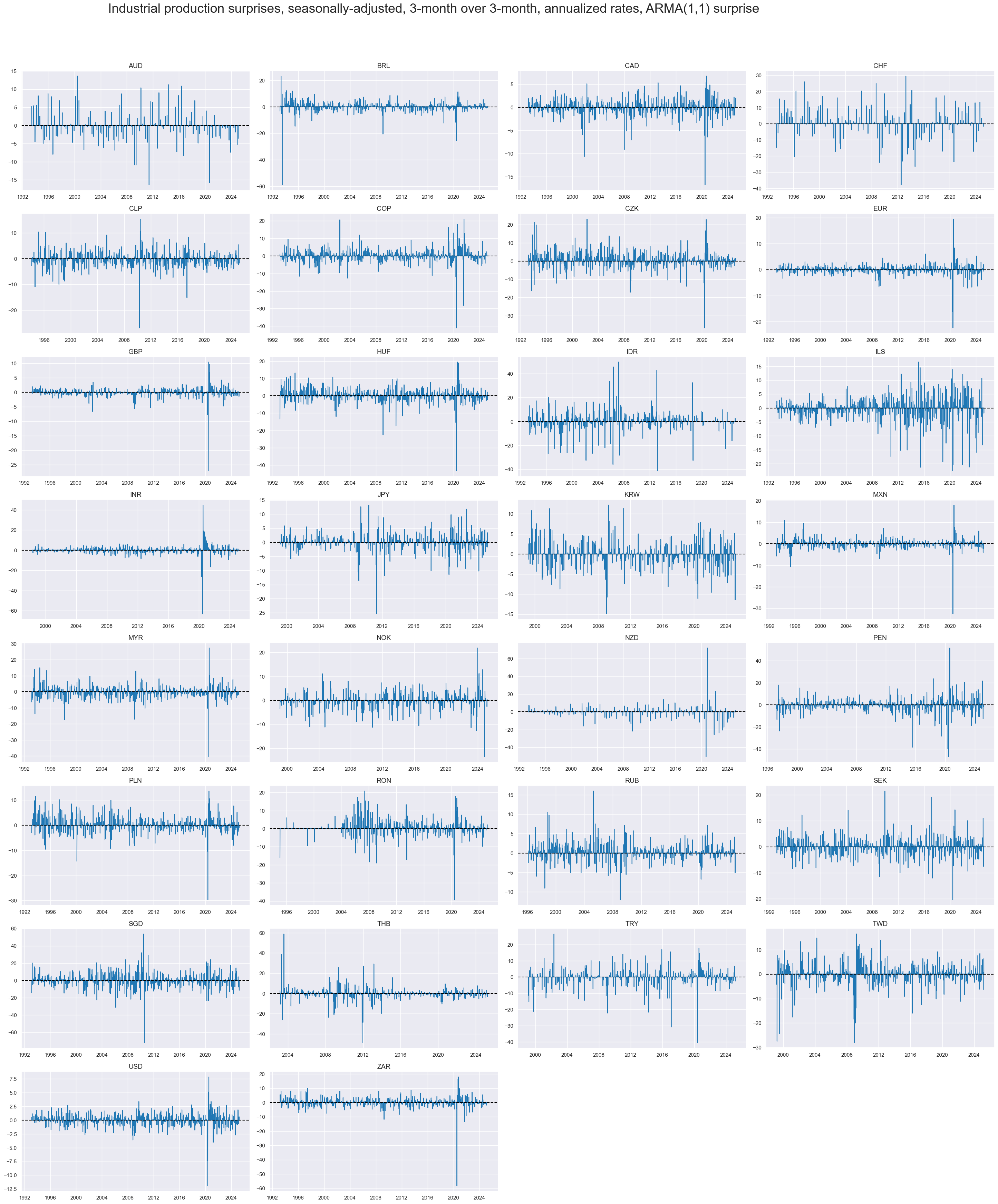
xcatx = ["IP_SA_P3M3ML3AR_ARMAS"]
cidx = sorted(list(set(cids_exp) - set(["PHP"])))

msp.view_timelines(
    dfd,
    xcats=xcatx,
    cids=cidx,
    start=start_date,
    title="Industrial production surprises, seasonally-adjusted, 3-month over 3-month, annualized rates, ARMA(1,1) surprise",
    title_adj=1.02,
    title_xadj=0.435,
    title_fontsize=27,
    legend_fontsize=17,
    label_adj=0.075,
    ncol=4,
    same_y=False,
    size=(12, 7),
    aspect=1.7,
    all_xticks=True,
)
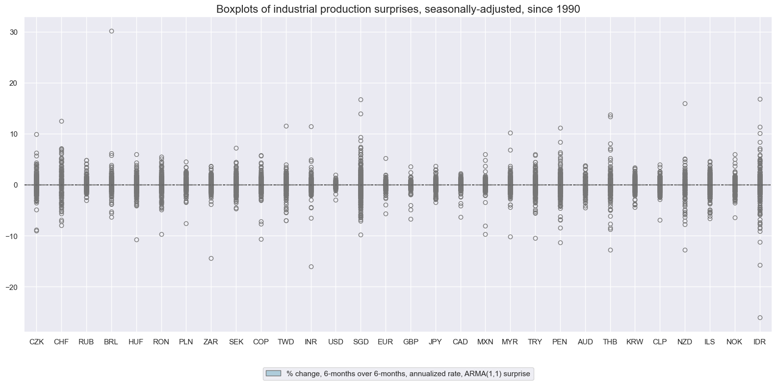
xcatx = ["IP_SA_P6M6ML6AR_ARMAS"]
cidx = list(set(cids_exp) - set(["PHP"]))


msp.view_ranges(
    dfd,
    xcats=xcatx,
    cids=cidx,
    sort_cids_by="mean",
    start=start_date,
    kind="box",
    title="Boxplots of industrial production surprises, seasonally-adjusted, since 1990",
    xcat_labels=["% change, 6-months over 6-months, annualized rate, ARMA(1,1) surprise",],
    size=(16, 8),
)
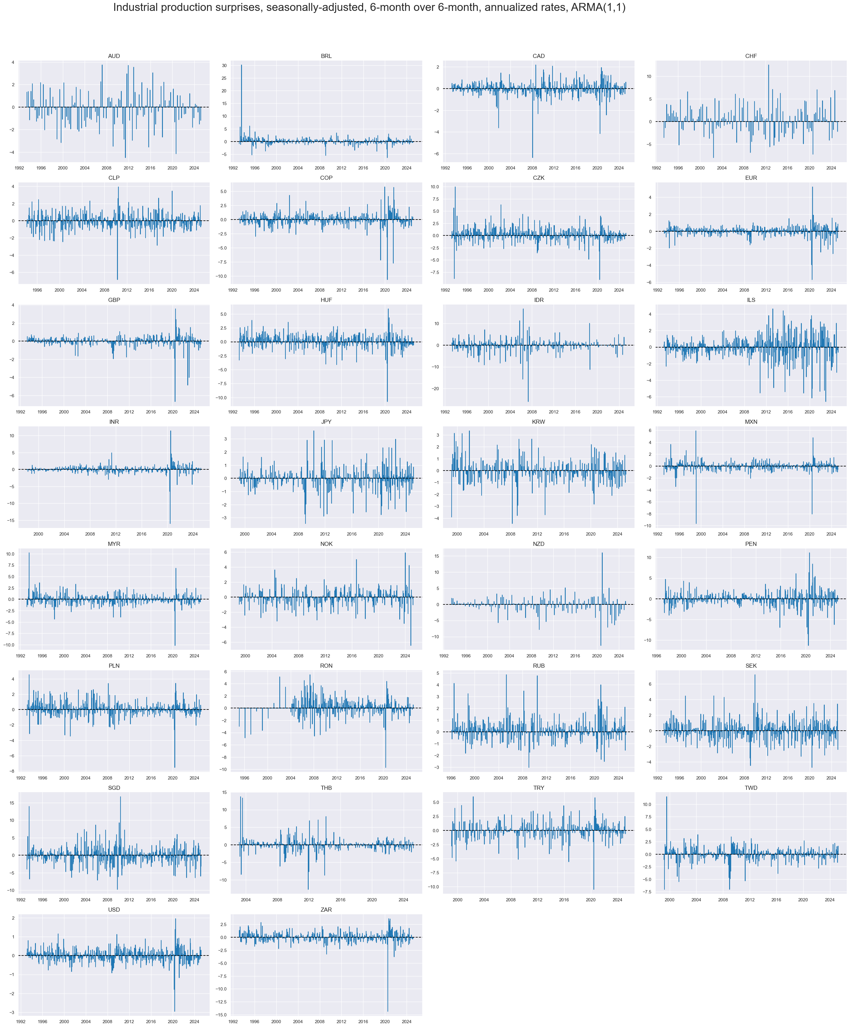
cids_appl = sorted(list(set(cids_exp) - set(["PHP"])))
xcatx = ["IP_SA_P6M6ML6AR_ARMAS"]
cidx = cids_appl

msp.view_timelines(
    dfd,
    xcats=xcatx,
    cids=cidx,
    start=start_date,
    title="Industrial production surprises, seasonally-adjusted, 6-month over 6-month, annualized rates, ARMA(1,1)",
    title_adj=1.02,
    title_xadj=0.435,
    title_fontsize=27,
    legend_fontsize=17,
    label_adj=0.075,
    ncol=4,
    same_y=False,
    size=(12, 7),
    aspect=1.7,
    all_xticks=True,
)
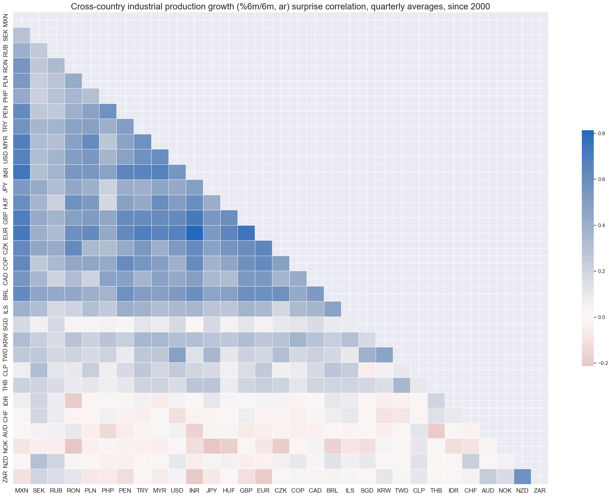
xcatx = "IP_SA_P6M6ML6AR_ARMAS"
cidx = cids_exp

msp.correl_matrix(
    dfd,
    xcats=xcatx,
    cids=cids_exp,
    freq="q",
    title="Cross-country industrial production growth (%6m/6m, ar) surprise correlation, quarterly averages, since 2000",
    cluster=True,
    size=(22, 16),
)
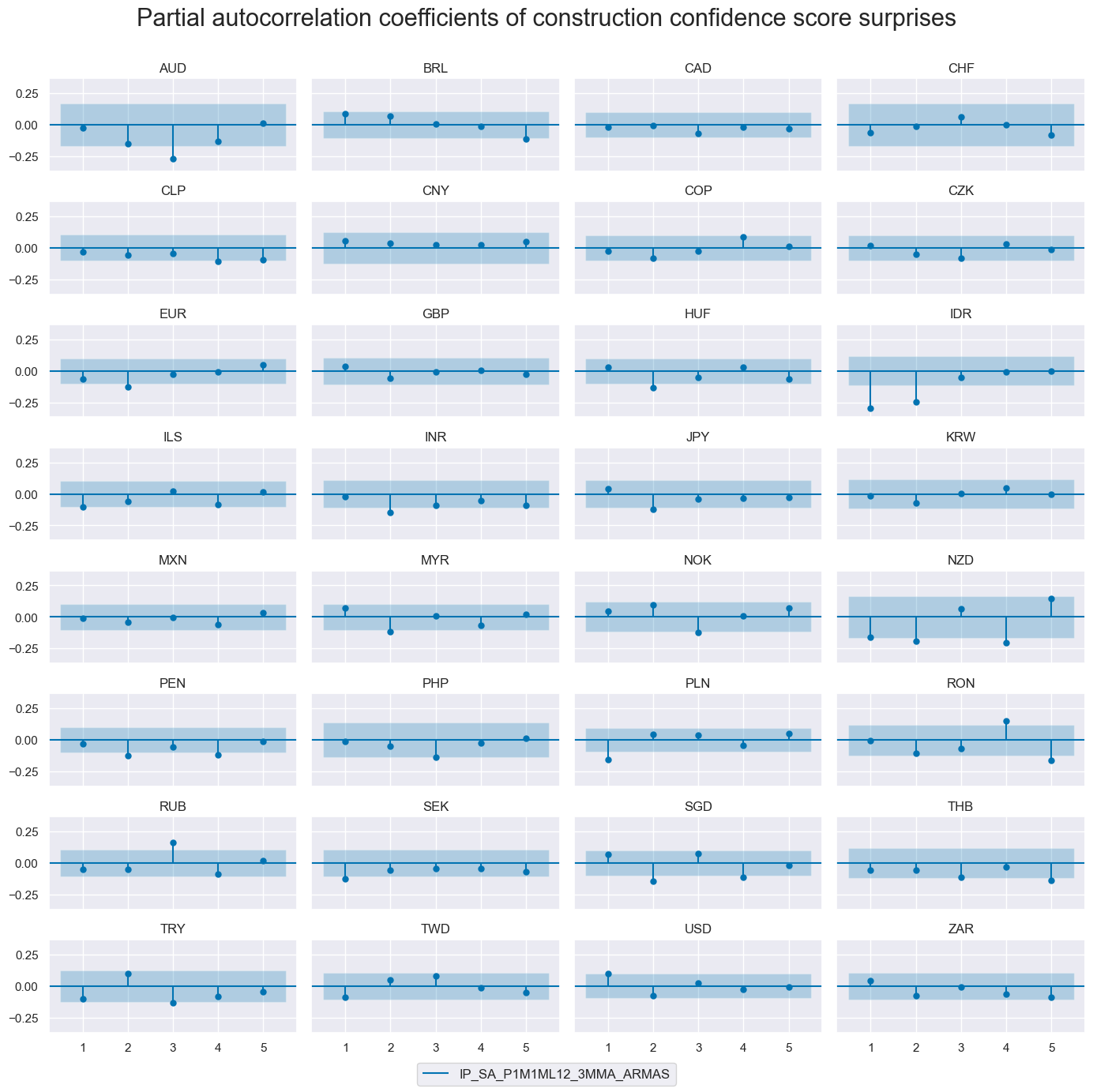
The autocorrelation (ACF) and partial autocorrelation (PACF) plots evaluate the temporal dependence of quantamental surprises across information events. Under the assumption of a well-specified prediction model of first-print releases and unbiased subsequent revisions, these surprises — interpreted as one-step-ahead forecast errors — should be serially uncorrelated.
cidx = sorted(cids_exp)

msv.plot_pacf(
    df=dfd,
    cids=cidx,
    xcat="IP_SA_P1M1ML12_3MMA_ARMAS",
    title="Partial autocorrelation coefficients of construction confidence score surprises",
    lags=5,
    remove_zero_predictor=True,
    figsize=(14, 14),
    ncols=4,
)
Importance #
Research links #
“Macroeconomic theory suggests that currencies of countries in a strong cyclical position should appreciate against those in a weak position. One metric for cyclical strength is the output gap, i.e. the production level relative to output at a sustainable operating rate.” Macrosynergy
Empirical clues #
# Normalization and winsorization of surprises (to make countries comparable)

xcatx = ["IP_SA_P3M3ML3AR_ARMAS", "IP_SA_P6M6ML6AR_ARMAS", "IP_SA_P1M1ML12_3MMA_ARMAS"]
cidx = list(set(cids_exp) - set(["PHP"]))

df_red = msm.reduce_df(dfd, xcats=xcatx, cids=cidx)

isc_obj = msm.InformationStateChanges.from_qdf(
    df=df_red,
    score_by="level"
)
dfa = isc_obj.to_qdf(value_column="zscore", postfix="N")

dfa["value"] = dfa["value"].clip(lower=-3, upper=3)
dfd = msm.update_df(dfd, dfa[["real_date", "cid", "xcat", "value"]])
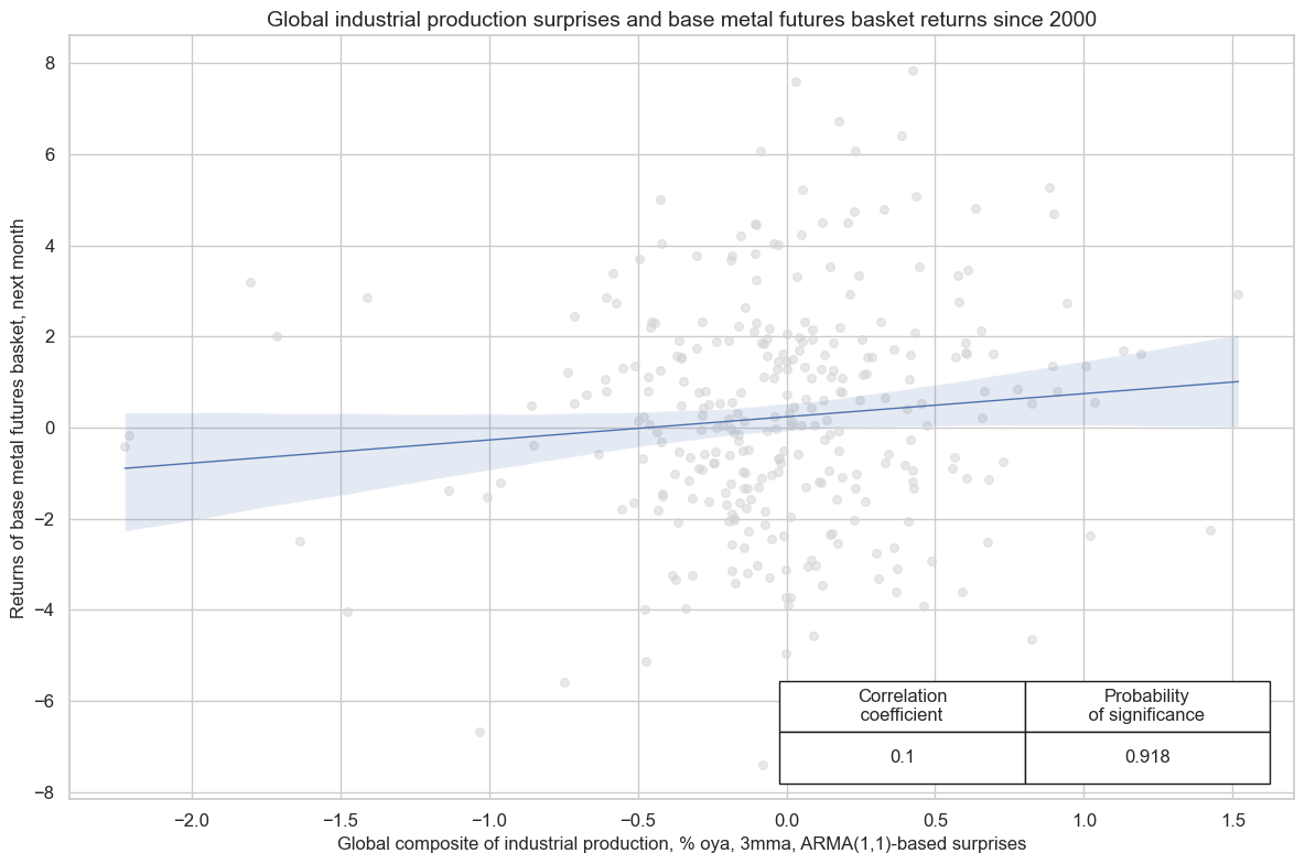
There is empirical evidence that global production-weighted industrial production surprises positively and significantly predict futures returns for a basket of industrial metals (aluminum, copper, lead, nickel, tin, and zinc) at monthly and quarterly frequencies.
cids_co = ["ALM", "CPR", "LED", "NIC", "TIN", "ZNC"]
cts = [cid + "_" for cid in cids_co]
bask_co = msp.Basket(dfd, contracts=cts, ret="COXR_VT10")
bask_co.make_basket(weight_meth="equal", basket_name="GLB")
dfa = bask_co.return_basket()

dfd = msm.update_df(dfd, dfa)  # Global industrial metals basket return
xcatx = [
    "IP_SA_P1M1ML12_3MMA_ARMASN",
    "IP_SA_P3M3ML3AR_ARMASN",
    "IP_SA_P6M6ML6AR_ARMASN"
]

for xc in xcatx:
    dfa = msp.linear_composite(
    df=dfd,
    xcats=xc,
    cids=cids,
    weights="IVAWGT_SA_1YMA",
    new_cid="GLB",
    complete_cids=False,
    )
    dfd = msm.update_df(dfd, dfa)
cr = msp.CategoryRelations(
    dfd,
    xcats=["IP_SA_P1M1ML12_3MMA_ARMASN", "COXR_VT10"],
    cids=["GLB"],
    freq="M",
    lag=1,
    xcat_aggs=["sum", "sum"],
    fwin=1,
    start="2000-01-01",
    years=None,
)

cr.reg_scatter(
    title="Global industrial production surprises and base metal futures basket returns since 2000",
    labels=False,
    coef_box="lower right",
    xlab="Global composite of industrial production, % oya, 3mma, ARMA(1,1)-based surprises",
    ylab="Returns of base metal futures basket, next month",
    remove_zero_predictor=True,
)
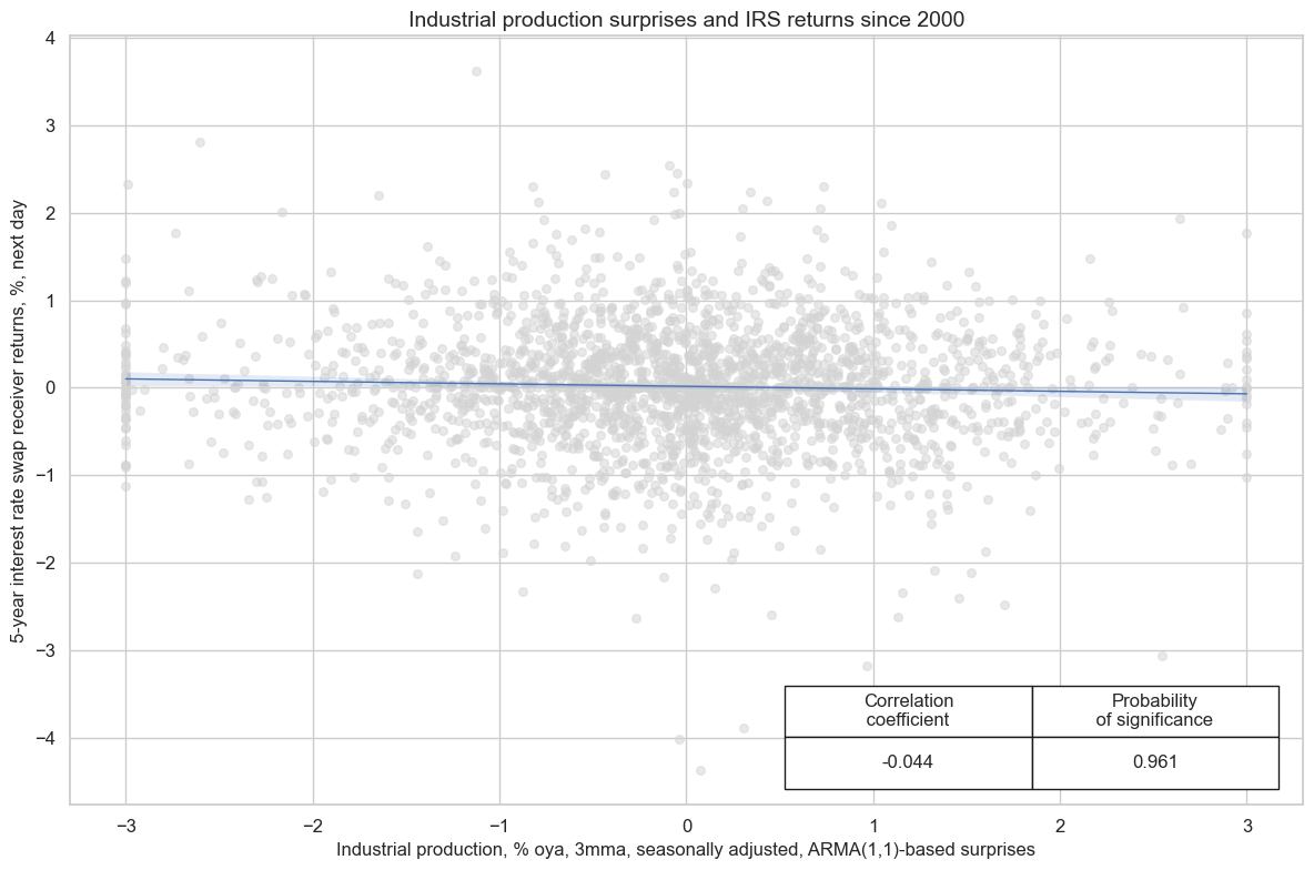
There is empirical evidence that industrial production surprises negatively predict the next day’s duration returns in developed countries.
cr = msp.CategoryRelations(
    dfd,
    xcats=["IP_SA_P1M1ML12_3MMA_ARMASN", "DU05YXR_VT10"],
    cids=cids_dmca,
    freq="D",
    lag=1,
    xcat_aggs=["sum", "sum"],
    fwin=1,
    start="2000-01-01",
    years=None,
    xcat_trims=[4, 8],
)

cr.reg_scatter(
    coef_box="lower right",
    title="Industrial production surprises and IRS returns since 2000",
    xlab="Industrial production, % oya, 3mma, seasonally adjusted, ARMA(1,1)-based surprises",
    ylab="5-year interest rate swap receiver returns, %, next day",
    prob_est="map",
    remove_zero_predictor=True,
)
Appendices #
Appendix 1: Currency symbols #
The word ‘cross-section’ refers to currencies, currency areas or economic areas. In alphabetical order, these are AUD (Australian dollar), BRL (Brazilian real), CAD (Canadian dollar), CHF (Swiss franc), CLP (Chilean peso), CNY (Chinese yuan renminbi), COP (Colombian peso), CZK (Czech Republic koruna), DEM (German mark), ESP (Spanish peseta), EUR (Euro), FRF (French franc), GBP (British pound), HKD (Hong Kong dollar), HUF (Hungarian forint), IDR (Indonesian rupiah), ITL (Italian lira), JPY (Japanese yen), KRW (Korean won), MXN (Mexican peso), MYR (Malaysian ringgit), NLG (Dutch guilder), NOK (Norwegian krone), NZD (New Zealand dollar), PEN (Peruvian sol), PHP (Phillipine peso), PLN (Polish zloty), RON (Romanian leu), RUB (Russian ruble), SEK (Swedish krona), SGD (Singaporean dollar), THB (Thai baht), TRY (Turkish lira), TWD (Taiwanese dollar), USD (U.S. dollar), ZAR (South African rand).
Appendix 2: Quantamental economic surprises #
Quantamental economic surprises are defined as deviations of point-in-time quantamental indicators from expected values. Expected values are estimated predictions of an informed market participant. Following this definition there are two types of surprises that jointly make up economic surprise indicators:
• A first print event is the difference between a quantamental indicator on a release date and its expected value. A release date is the day on which any underlying economic time series adds an observation period. Expected values are estimated, typically based on econometric models and information prior to the release date. A quantamental data surprise is always specific to the prediction model or statistical learning process.
• A pure revision event is the change in a quantamental indicator on a non-release date. It arises from revisions of data for previously released observation periods. Per default, it is assumed that all revisions are surprises, i.e., that the latest reported value for an observation period is the best predictor its value after revisions. Note that any revisions published on a release date become part of the first print event.
A quantamental indicator of economic surprises records the values of these two events on the dates they become known. It records zero values for all other dates. Models for predicting indicator values always use the latest vintage of the underlying data series. They are typically applied to increments, i.e., differences or log differences of volume, value or price indices. The predicted next increment produces an expected new vintage, and the expected new vintage implies a new derived expected quantamental indicator, such as an annual growth rate or moving average. Note than in this way predictions automatically account for “base effects”, i.e., predictable changes in growth rates that arise from unusually sharp increase of declines in index levels of the base period, for example a year ago.