Government debt sustainability

This category group contains “mechanical” general government debt sustainability metrics. They are very simple and highly stylized but popular for rough assessments. The calculation is based on the latest information states of debt and deficit ratios and estimates of the latest local-currency real government bond yields. As such, these ratios always assume that concurrent market conditions prevail going forward and are mostly an indication of the escalation risk of changes in credit and financial market conditions.

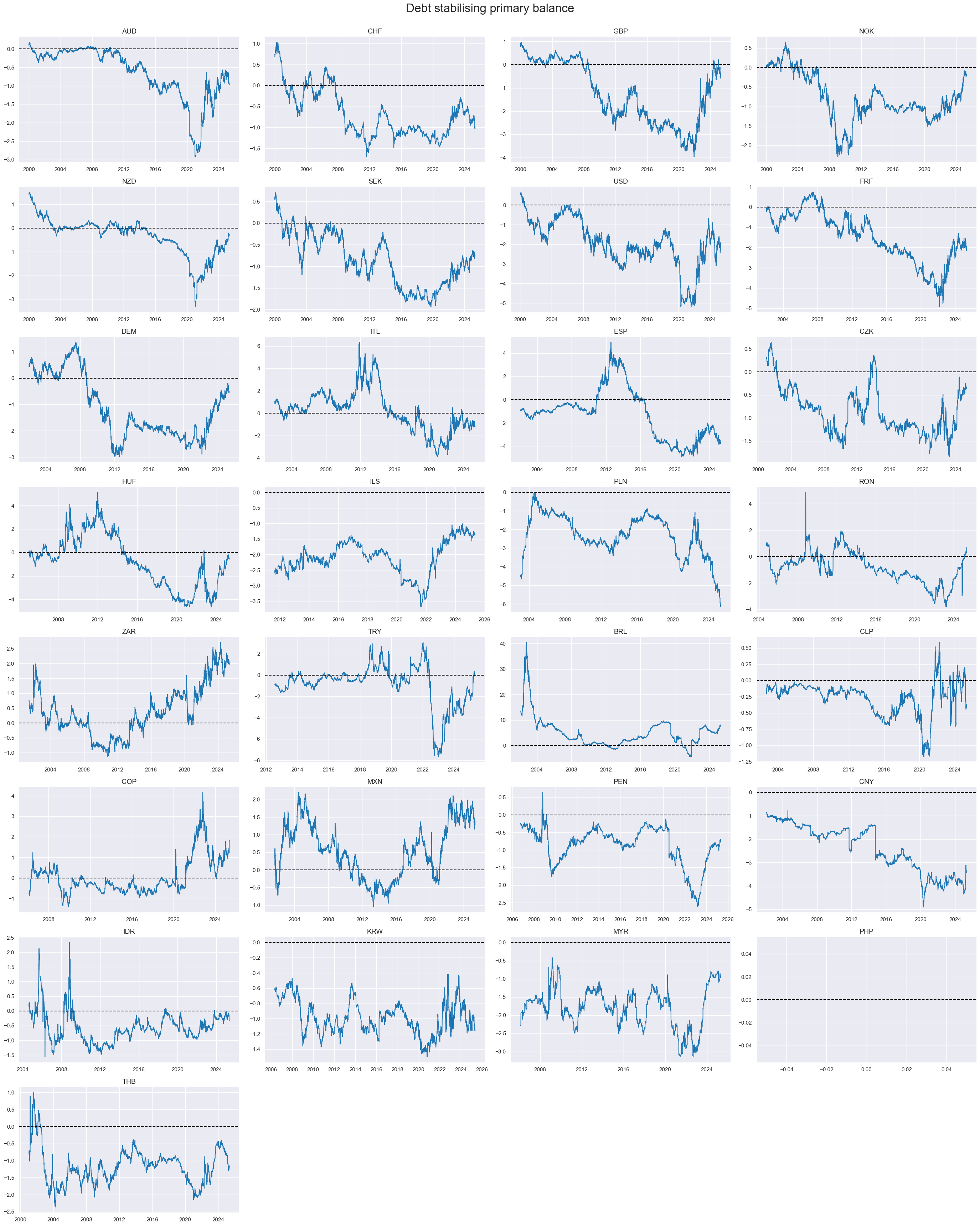
Debt-stabilising primary balance

Ticker : DSGGPBGDPRATIO_NSA

Label : Debt-stabilising general government primary balance, % of GDP.

Definition : General government’s primary balance as % of GDP for the current year that would imply stable government debt ratios going forward.

Notes :

• The primary government balance is the difference between government revenues and expenditures, excluding debt service.

• The debt-stabilizing primary balance ratio is a threshold ratio below which the general government debt-to-GDP ratio would be rising and above which it would be decreasing. For example, if that ratio is a large surplus, the government would have to collect much higher revenues than the funds it can spend.

• The daily information states of this ratio assume that estimate real interest rates are representative of future debt servicing costs and do not change in the future.

• The exact calculations of this ratio can be found in the first section of Appendix 1 .

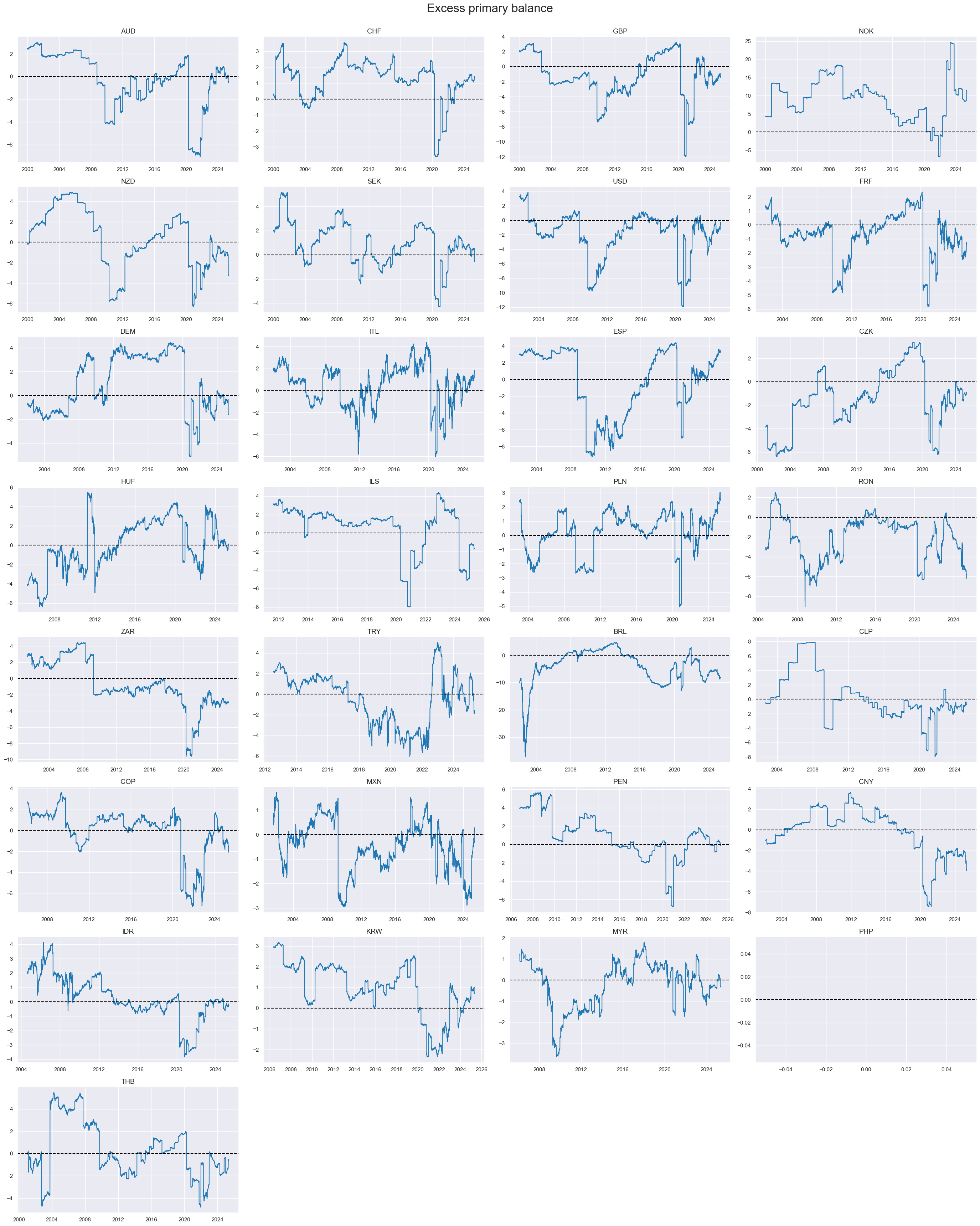
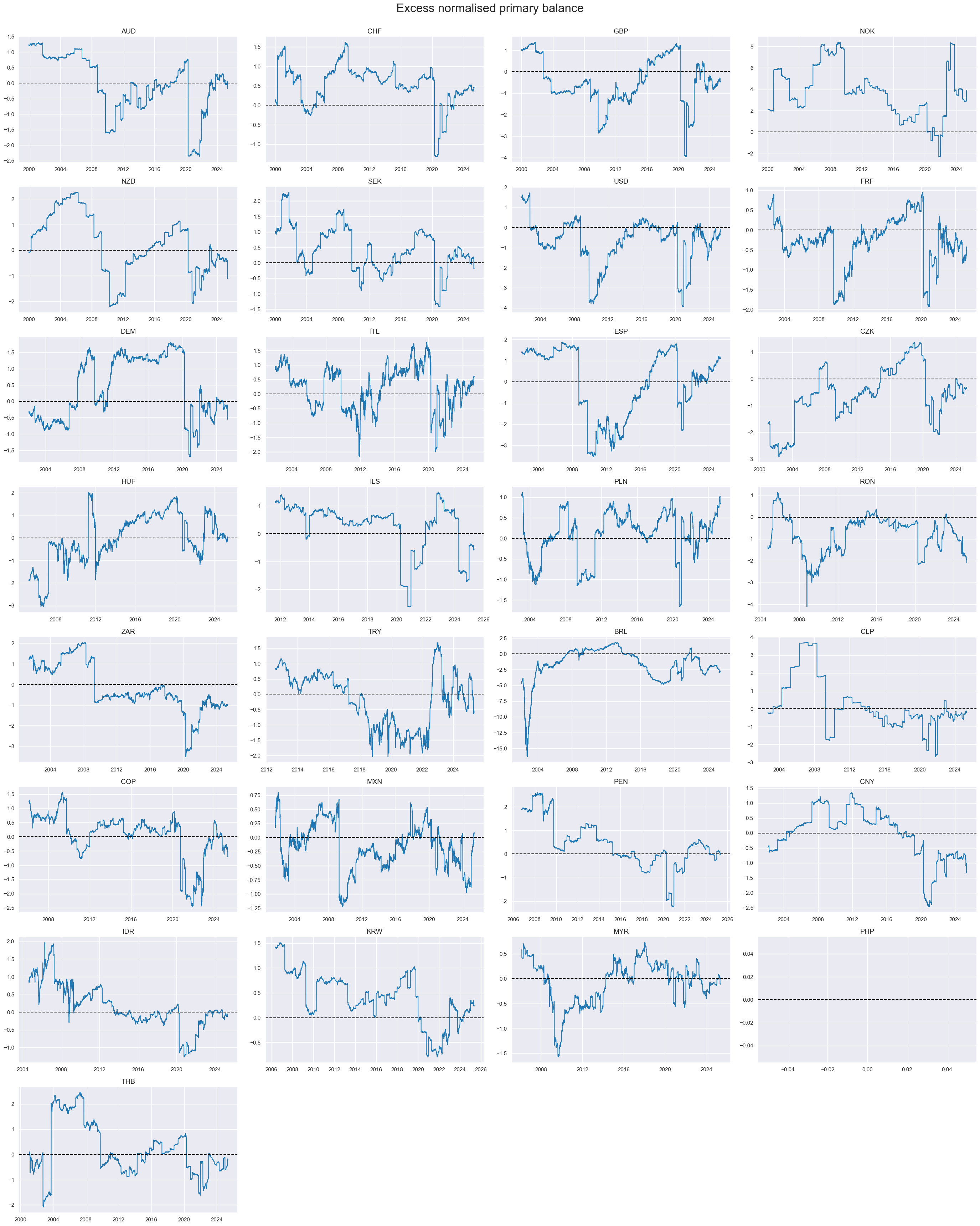
Excess primary balance

Ticker : XGGPBGDPRATIO_NSA / XNGGPBGDPRATIO_NSA

Label : Excess general government primary balance, % of GDP / Excess general government primary balance, normalized

Definition : Expected primary balance ratio (% of GDP) minus debt-stabilising general government primary balance / Normalized expected primary balance ratio (% of GDP) minus debt-stabilising general government primary balance

Notes :

• These indicators take the difference of two information states: the estimated general government primary balance ratio and the estimated debt-stabilizing primary balance ratio. A positive value suggests that the current estimated balance implies declining debt ratios. A negative value suggests that the current estimated balance implies rising general government debt ratios.

• These excess balance indicate how much fiscal policy can ease before the balance reaches a debt-increasing threshold (for positive excess ratios) or how much it must tighten before it reaches a debt stabilizing threshold (for shortfalls)

• The normalized excess balances divide the excess primary balances by an estimate of standard deviations of primary balances based on a global panel of data available point-in-time. They allow an assessment of the effort that is required to attain the debt-stabilizing primary balance under consideration of normal variability of fiscal policy.

• Calculations can be found in the first and second part of Appendix 1 .

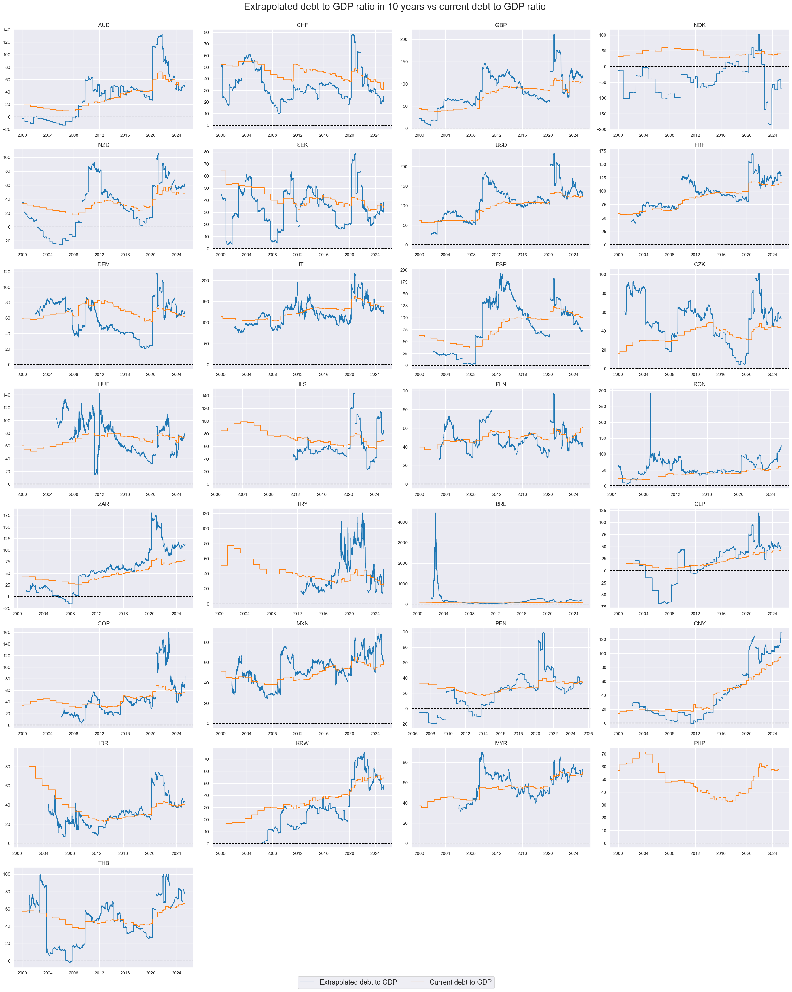
Extrapolated debt ratio in 10 years

Ticker : GGDGDPRATIOX10_NSA

Label : Extrapolated debt-to-GDP ratio in 10 years.

Definition : Extrapolated general government debt-to-GDP ratio in 10 years, given the current primary balance, real interest rate estimates, and concurrent general government debt ratio.

Notes :

• This indicator indicates, ceteris paribus, where the debt-to-GDP ratio of a government would reach, if interest rates, GDP growth and the primary balanced remained unchanged.

• This is a metric of fiscal and debt escalation risk, where fear of default and rising bond yields move into mutually reinforcing dynamics.

• Calculations can be found in Appendix 1 .

Imports

Only the standard Python data science packages and the specialized macrosynergy package are needed.

import os
import numpy as np
import pandas as pd
from pandas import Timestamp
import matplotlib.pyplot as plt
import seaborn as sns

import warnings
from datetime import timedelta, date

import macrosynergy.management as msm
import macrosynergy.panel as msp
import macrosynergy.signal as mss
import macrosynergy.pnl as msn
from macrosynergy.download import JPMaQSDownload

import requests
from timeit import default_timer as timer

warnings.simplefilter("ignore")

The JPMaQS indicators we consider are downloaded using the J.P. Morgan Dataquery API interface within the macrosynergy package. This is done by specifying ticker strings , formed by appending an indicator category code <category> to a currency area code <cross_section> . These constitute the main part of a full quantamental indicator ticker, taking the form DB(JPMAQS,<cross_section>_<category>,<info>) , where <info> denotes the time series of information for the given cross-section and category.

The following types of information are available:

• value giving the latest available values for the indicator

• eop_lag referring to days elapsed since the end of the observation period

• mop_lag referring to the number of days elapsed since the mean observation period

• grade denoting a grade of the observation, giving a metric of real time information quality.

After instantiating the JPMaQSDownload class within the macrosynergy.download module, one can use the download(tickers, start_date, metrics) method to obtain the data. Here tickers is an array of ticker strings, start_date is the first release date to be considered and metrics denotes the types of information requested.

# Cross-sections of interest

cids_dmca = ["AUD", "CHF", "GBP", "NOK", "NZD", "SEK", "USD"]
cids_dmeu = [
    "FRF",
    "DEM",
    "ITL",
    "ESP",
]  # DM euro area sovereigns
cids_latm = [
    "BRL",
    "CLP",
    "COP",
    "MXN",
    "PEN",
]  # Latam sovereigns
cids_emea = [
    "CZK",
    "HUF",
    "ILS",
    "PLN",
    "RON",
    "ZAR",
    "TRY",
]  # EMEA sovereigns
cids_emas = [
    "CNY",
    "IDR",
    "KRW",
    "MYR",
    "PHP",
    "THB",
]  # EM Asia sovereigns

cids_dm = cids_dmca + cids_dmeu
cids_em = cids_emea + cids_latm + cids_emas

cids = cids_dm + cids_em

debtsus = ['DSGGPBGDPRATIO_NSA', 'XGGPBGDPRATIO_NSA', 'XNGGPBGDPRATIO_NSA', 'GGDGDPRATIOX10_NSA']

gov_fin = ['GGDGDPRATIO_NSA'] # Debt
govs = ["GB02YYLD_NSA", "GB05YYLD_NSA", "GB10YYLD_NSA"]
rets = ["GB02YR_NSA", "GB05YR_NSA", "GB10YR_NSA", "CDS05YXR_VT10", "CDS05YXR_NSA"]
cds = ["CDS05YXRxEASD_NSA", "CDS05YXRxLEV10_NSA"]

main = debtsus
mkts = gov_fin + govs + rets + cds
xcats = main + mkts

# Download series from J.P. Morgan DataQuery by tickers

start_date = "1996-01-01"
tickers = [cid + "_" + xcat for cid in cids for xcat in xcats]
print(f"Maximum number of tickers is {len(tickers)}")

# Retrieve credentials

oauth_id = os.getenv("DQ_CLIENT_ID")  # Replace with own client ID
oauth_secret = os.getenv("DQ_CLIENT_SECRET")  # Replace with own secret

with JPMaQSDownload(client_id=oauth_id, client_secret=oauth_secret) as downloader:
    start = timer()
    df = downloader.download(
        tickers=tickers,
        start_date=start_date,
        metrics=["value", "eop_lag", "mop_lag", "grading"],
        suppress_warning=True,
        show_progress=True,
    )
    end = timer()

dfd = df

print("Download time from DQ: " + str(timedelta(seconds=end - start)))

Maximum number of tickers is 435
Downloading data from JPMaQS.
Timestamp UTC:  2024-07-18 18:55:20
Connection successful!

Requesting data: 100%|██████████| 87/87 [00:18<00:00,  4.68it/s]
Downloading data: 100%|██████████| 87/87 [00:12<00:00,  6.87it/s]

Some expressions are missing from the downloaded data. Check logger output for complete list.
524 out of 1740 expressions are missing. To download the catalogue of all available expressions and filter the unavailable expressions, set `get_catalogue=True` in the call to `JPMaQSDownload.download()`.
Some dates are missing from the downloaded data. 
3 out of 7451 dates are missing.
Download time from DQ: 0:00:35.487050

Availability

cids_exp = sorted(list(cids))  # cids expected in category panels
msm.missing_in_df(dfd, xcats=main, cids=cids_exp)

Missing xcats across df:  []
Missing cids for DSGGPBGDPRATIO_NSA:  ['PHP']
Missing cids for GGDGDPRATIOX10_NSA:  ['PHP']
Missing cids for XGGPBGDPRATIO_NSA:  ['PHP']
Missing cids for XNGGPBGDPRATIO_NSA:  ['PHP']

Starting dates for sovereign CDS volatilities are mixed. For most cross-sections, data is available only from the mid-2000s onwards. The only countries for which data are available from the 1990s are Brazil, Colombia, Mexico and Poland.

For the explanation of currency symbols, which are related to currency areas or countries for which categories are available, please view Appendix 1 .

xcatx = main
cidx = cids_exp

dfx = msm.reduce_df(dfd, xcats=xcatx, cids=cidx)
dfs = msm.check_startyears(
    dfx,
)
msm.visual_paneldates(dfs, size=(24, 4))

print("Last updated:", date.today())

Last updated: 2023-10-06

xcatx = main
cidx = cids_exp

plot = msm.check_availability(
    dfd, xcats=xcatx, cids=cidx, start_size=(18, 3), start_years=False
)

xcatx = main
cidx = cids_exp

plot = msp.heatmap_grades(
    dfd,
    xcats=xcatx,
    cids=cidx,
    size=(18, 3),
    title=f"Average vintage grades from {start_date} onwards",
)

History

Debt-stabilising primary balance ratios

xcatx = ['DSGGPBGDPRATIO_NSA' ]
cidx = cids

msp.view_timelines(
    dfd,
    xcats=xcatx,
    cids=cidx,
    start="2000-01-01",
    title="Debt stabilising primary balance",
    title_fontsize=24,
    legend_fontsize=17,
    xcat_labels=["PB"],
    ncol=4,
    same_y= False,
    all_xticks=True
)

Excess primary balance ratios

xcatx = ['XGGPBGDPRATIO_NSA']
cidx = cids

msp.view_timelines(
    dfd,
    xcats=xcatx,
    cids=cidx,
    start="2000-01-01",
    title="Excess primary balance",
    title_fontsize=24,
    legend_fontsize=17,
    xcat_labels=["PB"],
    ncol=4,
    same_y= False,
    all_xticks=True
)

Normalised excess primary balance ratios

xcatx = ['XNGGPBGDPRATIO_NSA']
cidx = cids

msp.view_timelines(
    dfd,
    xcats=xcatx,
    cids=cidx,
    start="2000-01-01",
    title="Excess normalised primary balance",
    title_fontsize=24,
    legend_fontsize=17,
    xcat_labels=["PB"],
    ncol=4,
    same_y= False,
    all_xticks=True
)

Extrapolated debt ratios

xcatx = ['GGDGDPRATIOX10_NSA', 'GGDGDPRATIO_NSA']
cidx = cids

msp.view_timelines(
    dfd,
    xcats=xcatx,
    cids=cidx,
    start="2000-01-01",
    title="Extrapolated debt to GDP ratio in 10 years vs current debt to GDP ratio ",
    title_fontsize=24,
    legend_fontsize=17,
    xcat_labels=["Extrapolated debt to GDP", "Current debt to GDP"],
    ncol=4,
    same_y= False,
    all_xticks=True
)

Importance

Relevant research

“In practical terms, debt is sustainable if increases in this ratio are reverted in the medium and long term. Thus, debt sustainability reduces the risk of default and avoids the negative externalities associated with high debt levels. The risk of default depends on expected future debt levels. With high expected debt levels the probability of ending up in a self-fulfilling vicious circle increases (Padoan et al., 2012)—i.e. high government debt leads to an increase in risk premia, implying a higher discount rate for future government surpluses which justifies these higher risk premia. Given higher interest rates, current cash flow becomes more important relative to future cash flow limiting the sovereign’s options to increase its surplus. When the market anticipates these rates will become so high that the government is no longer willing to take the actions necessary to repay its debt, the country will be excluded from the international capital market altogether: a liquidity crisis, possibly followed by a default, emerges” Jasper Lukkezen, Hugo Rojas-Romagosa

“Furthermore, high debt levels themselves, and not only their anticipation, have empirically well-established detrimental effects on the economy: they lower future economic growth (Reinhart and Rogoff, 2010; Kumar and Woo, 2012; Baum et al., 2012), may crowd-out private investment (Kumar and Woo, 2012) and increase the interest payments necessary to service the debt (Bayoumi et al., 1995; Schuknecht et al., 2009).” Jasper Lukkezen, Hugo Rojas-Romagosa

“However, other economists challenged this view, putting into evidence the reversibility of the current low interest rate environment and highlighting that debt was not a ‘free lunch’. Specific individual levels of ‘r’ and ‘g’ are likely to matter more for sustainable debt dynamics than the difference between them. Large and positive GDP growth is especially important: when growth is low or suddenly plunges, this hampers the government’s ability to increase the primary balance or to undertake structural reforms to boost long-term growth (e.g. it is politically challenging to fiscally adjust/cut spending when incomes are stagnant). Moreover, despite favourable financing conditions prevailing, spreads remain in EU countries, reflecting different fundamental characteristics (180), and history has shown that financial markets can react quickly and abruptly to changes in economic circumstances (181).” European Commission

Empirical clues

There has been modest but signficant positive correlation between changes in excess primary balances and subsequent CDS returns across DM and EM at a quarterly frequency.

xcatx = ["XNGGPBGDPRATIO_NSA", "CDS05YXR_NSA"] 
cidx = cids

crx = msp.CategoryRelations(
    dfd,
    xcats=xcatx,
    xcat1_chg="diff",
    cids=cidx,
    freq="Q", 
    lag=1,
    xcat_aggs=["last","sum"],
    start="2000-01-01",
    end=None,
    xcat_trims=[10, 5]
)
crx.reg_scatter(
    labels=False,
    coef_box="lower left",
    xlab="Excess primary balance, normalized, change over quarter",
    ylab="5-year CDS return, next quarter",
    title="Excess primary balance and subsequent 5-year CDS returns", 
    prob_est="map"
)

XNGGPBGDPRATIO_NSA misses: ['PHP'].

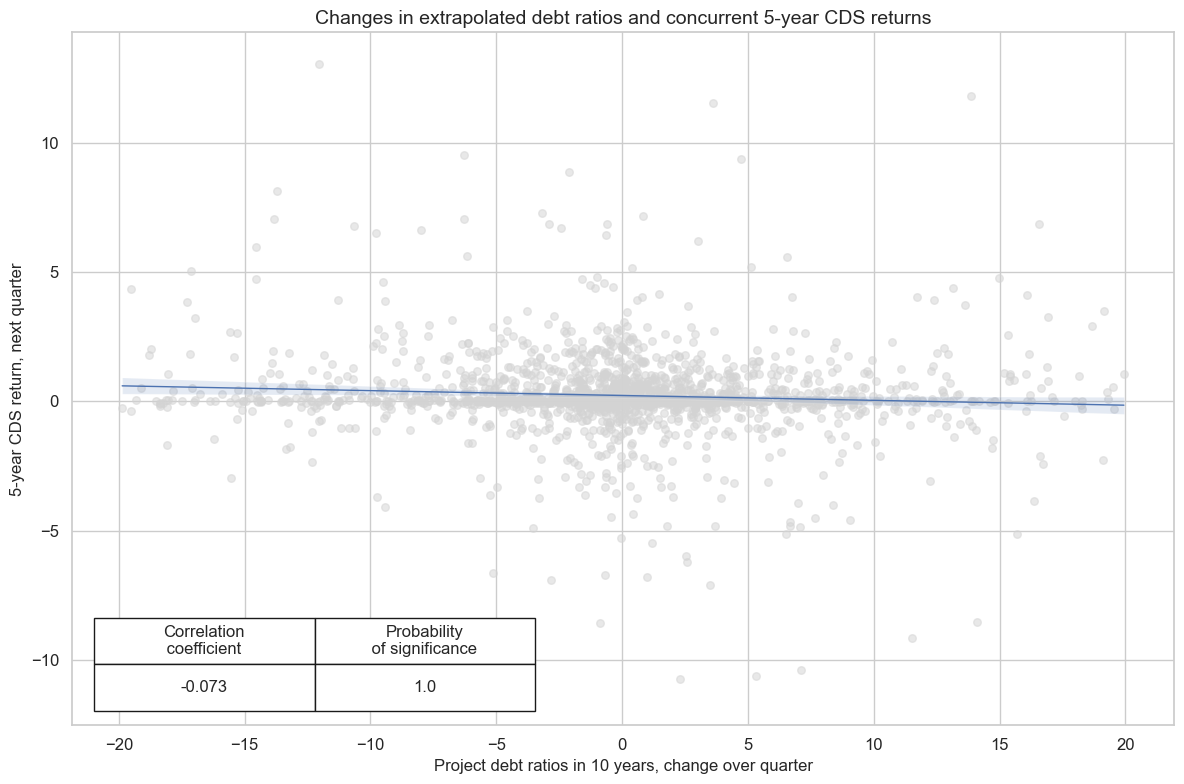
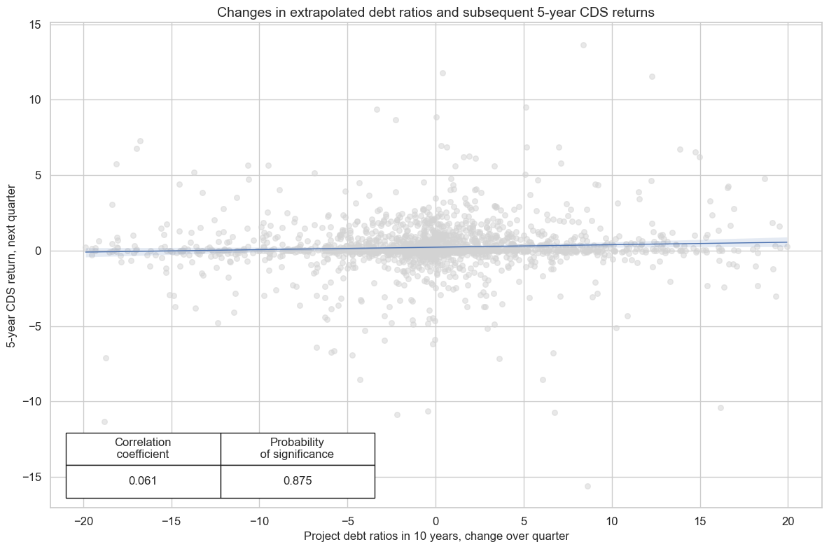
There is some slight evidence of “panic payback” for projected debt dynamics in CDS markets, as there is a strong negative concurrent relation between extrapolated debt ratio changes and a positive subsequent relation.

xcatx = ["GGDGDPRATIOX10_NSA", "CDS05YXR_NSA"] 
cidx = cids

crx = msp.CategoryRelations(
    dfd,
    xcats=xcatx,
    xcat1_chg="diff",
    cids=cidx,
    freq="Q", 
    lag=0,
    xcat_aggs=["last","sum"],
    start="2000-01-01",
    end=None,
    xcat_trims=[20, 50]  # outlier
)
crx.reg_scatter(
    labels=False,
    coef_box="lower left",
    xlab="Project debt ratios in 10 years, change over quarter",
    ylab="5-year CDS return, next quarter",
    title="Changes in extrapolated debt ratios and concurrent 5-year CDS returns", 
    prob_est="map"
)

GGDGDPRATIOX10_NSA misses: ['PHP'].

xcatx = ["GGDGDPRATIOX10_NSA", "CDS05YXR_NSA"] 
cidx = cids

crx = msp.CategoryRelations(
    dfd,
    xcats=xcatx,
    xcat1_chg="diff",
    cids=cidx,
    freq="Q", 
    lag=1,
    xcat_aggs=["last","sum"],
    start="2000-01-01",
    end=None,
    xcat_trims=[20, 50]  # outlier
)
crx.reg_scatter(
    labels=False,
    coef_box="lower left",
    xlab="Project debt ratios in 10 years, change over quarter",
    ylab="5-year CDS return, next quarter",
    title="Changes in extrapolated debt ratios and subsequent 5-year CDS returns", 
    prob_est="map"
)

GGDGDPRATIOX10_NSA misses: ['PHP'].

Appendices

Appendix 1: Calculation of stylized debt sustainability indicators

Debt-stabilizing primary balances and excess primary balances

The stylized debt sustainability metrics in JPMaQS follow conventions used by economists for decades and are summarized for example in a research paper by Olivier Blanchard. In a simple stylized model the dynamics of the general government debt-to-GDP ratio (d) is assumed to be governed by a simple first order difference equation:

(1) \[\begin{equation} d_{t+1} = {\frac{1+r}{1+g}}(d_{t}-s_{t}) \end{equation}\]

where r is defined as the real interest rate paid on outstanding debt, g is the medium-term rate of GDP growth, d is the government’s debt to GDP ratio at time t and s is the government’s primary balance/deficit to GDP ratio.

The real interest rate payable on government debt in the future is approximated based on structure and available data across countries. For most countries, it is through the estimated government bond 5 year real yields. For CHF, ZAR, INR and KRW we approximate the cost of debt with 5-year real interest rate swap yields. For a small number of countries (BRL, MYR, PEN, RON), we approximate with the sum of the real short term interest rate and the respective CDS spread.

We approximate the medium-term GDP growth with the quantamental indicator of 5-year median GDP growth rates (RGDP_SA_P1Q1QL4_20QMM) with the documentation here

Re-arranging the above equation we obtain an expression for the rate of change of the debt ratio:

(2) \[\begin{equation} d_{t+1} - d_{t} = {\frac{r-g}{1+g}}*d_{t}-s_{t} \end{equation}\]

If one requires the debt increase to be zero, one gets the stylized debt-stabilizing primary balance (pb):

(3) \[\begin{equation} \hat{pb_{t}} = {\frac{r-g}{1+g}}*d_{t} \end{equation}\]

One notices that, in the case of (r-g) < 0, the government does not need to run a primary surplus to stabilise debt. In fact, it can run a primary deficit. Rather surprisingly, the larger the debt ratio, the larger the primary deficit it can run while maintaining the debt ratio stable.

Subsequently, we calculate the excess primary balance , which is the difference between the current year’s expected primary balance and the debt-stabilizing primary balance. The current year’s primary balance is taken from another category group of JPMaQS indicators, with the documentation here

(4) \[\begin{equation} xpb_{t} = pb_{t} - \hat{pb_{t}} \end{equation}\]

Normalised excess primary balance

Normalization here means that we express excess balances in terms of standard deviations of such balances across all countries prior to the observation of their concurrent information states. This gives a better idea of the strength of fiscal effort that would be required for stabilizing the dynamics of public finances.

The first step is to calculate the historical standard deviation of each country’s primary balance:

(5) \[\begin{equation} sd_{i,pb} = \sqrt{\frac{1}{n-1} \sum_{j=1}^n (pb_i - \overline{pb_{i}})^2} \end{equation}\]

Where n is the number of years in our observation range, i is the country. We then calculate the average of these across the panel, where i corresponds to country i in the subset of k countries:

(6) \[\begin{equation} \overline{sd_{pb}} = \sum_{i=1}^{k}sd_{i,pb} * \frac{1}{k} \end{equation}\]

Then we can calculate the normalised excess primary balance, for each country as a ratio of its excess primary balance ratio to the panel standard deviation.

(7) \[\begin{equation} nxpb_{i, t} = \frac{xpb_{i,t}}{\overline{sd_{pb}}} \end{equation}\]

Extrapolated debt ratio in 10 years

We calculate a theoretical 10-year ahead general government debt-to-GDP ratio arising from the drift of the debt to GDP ratio, assuming that all other variables (the real GDP growth, the real cost of debt and the primary balance) stay the same across the 10-year period. To extrapolate the debt to GDP ratio in 10 years, we use the following recursive formula for the debt one year ahead, which we apply 10 times.

(8) \[\begin{equation} K = {\frac{r-g}{1+g}} \end{equation}\]

(9) \[\begin{equation} d_{t+1} = \sum_{t=1}^{10}{K}*d_{t}-s_{t}+d_{t} \end{equation}\]