Foreign trade trends

Foreign trade trends #

This category group contains real-time measures of trends in foreign trade flows. The measures are based on both actual and estimated vintages of exports and imports denominated in local currencies. Trends are extracted as filtered changes of latest vintages of seasonally and calendar-adjusted values. They are often indicative of domestic and external demand.

Merchandise export trends #

Ticker : EXPORTS_SA_P3M3ML3AR / _P6M6ML6AR / _P1M1ML12 / _P1M1ML12_3MMA

Label : Export values, seasonally and calendar adjusted: % 3m/3m ar / % 6m/6m ar / % oya / % oya 3mma

Definition : Merchandise exports in local currency, adjusted for seasonal effects, working days and holidays: % of latest 3 months over previous 3 months at an annualized rate / % of latest 6 months over previous 6 months at an annualized rate / % over a year ago / % over a year ago, 3-month moving average

Notes :

Data are taken from external merchandise trade statistics of either the balances of payment or customs trade statistics.
Seasonal adjustment factors are sequentially re-estimated as new data is being released. Every re-estimation gives rise of a new data vintage which is the basis of concurrent trend estimation.
For most countries, calendar adjustment is applied, accounting for working day effects and moving holidays (e.g. Chinese New Year, Easter, Diwali, Ramadan).
The national sources series’ have been complemented with additional vintages provided by OECD’s ‘Revision Analysis’ dataset. See also Appendix 1 for details on OECD data integration.

Merchandise import trends #

Ticker : IMPORTS_SA_P3M3ML3AR / _P6M6ML6AR / _P1M1ML12 / _P1M1ML12_3MMA

Label : Import value, seasonally and calendar adjusted: % 3m/3m ar / % 6m/6m ar / % oya / % oya 3mma

Definition : Merchandise imports in local currency, adjusted for seasonal effects, working days and holidays: % of latest 3 months over previous 3 months at an annualized rate / % of latest 6 months over previous 6 months at an annualized rate / % over a year ago / % over a year ago, 3-month moving average

Notes :

Data are taken from external merchandise trade statistics of either the balances of payment or customs trade statistics.
Seasonal adjustment factors are sequentially re-estimated as new data are being released. Every re-estimation gives rise of a new data vintage which is the basis of concurrent trend estimation.
For most countries, calendar adjustment is applied, accounting for working day effects and moving holidays (e.g. Chinese New Year, Easter, Diwali, Ramadan).
The national sources series’ have been complemented with additional vintages provided by OECD’s ‘Revision Analysis’ dataset. See also Appendix 1 for details on OECD data integration.

Imports #

Only the standard Python data science packages and the specialized macrosynergy package are needed.

             import os
import numpy as np
import pandas as pd
import matplotlib.pyplot as plt
import seaborn as sns
import math

import json
import yaml

import macrosynergy.management as msm
import macrosynergy.panel as msp
import macrosynergy.signal as mss
import macrosynergy.pnl as msn


from macrosynergy.download import JPMaQSDownload

from timeit import default_timer as timer
from datetime import timedelta, date, datetime

import warnings

warnings.simplefilter("ignore")

            

The JPMaQS indicators we consider are downloaded using the J.P. Morgan Dataquery API interface within the macrosynergy package. This is done by specifying ticker strings , formed by appending an indicator category code <category> to a currency area code <cross_section> . These constitute the main part of a full quantamental indicator ticker, taking the form DB(JPMAQS,<cross_section>_<category>,<info>) , where <info> denotes the time series of information for the given cross-section and category.

The following types of information are available:

value giving the latest available values for the indicator
eop_lag referring to days elapsed since the end of the observation period
mop_lag referring to the number of days elapsed since the mean observation period
grade denoting a grade of the observation, giving a metric of real time information quality.

After instantiating the JPMaQSDownload class within the macrosynergy.download module, one can use the download(tickers, start_date, metrics) method to obtain the data. Here tickers is an array of ticker strings, start_date is the first release date to be considered and metrics denotes the types of information requested.

             # Cross-sections of interest

cids_dmca = [
    "AUD",
    "CAD",
    "CHF",
    "EUR",
    "GBP",
    "JPY",
    "NOK",
    "NZD",
    "SEK",
    "USD",
]  # DM currency areas
cids_dmec = ["DEM", "ESP", "FRF", "ITL", "NLG"]  # DM euro area countries
cids_latm = ["BRL", "COP", "CLP", "MXN", "PEN"]  # Latam countries
cids_emea = ["HUF", "ILS", "PLN", "RON", "RUB", "TRY", "ZAR"]  # EMEA countries
cids_emas = [
    "CNY",
    "HKD",
    "IDR",
    "INR",
    "KRW",
    "MYR",
    "PHP",
    "SGD",
    "THB",
    "TWD",
]  # EM Asia countries

cids_dm = cids_dmca + cids_dmec
cids_em = cids_latm + cids_emea + cids_emas

cids = sorted(cids_dm + cids_em)

            

             # Quantamental categories of interest

exps = [
    "EXPORTS_SA_P1M1ML12",
    "EXPORTS_SA_P1M1ML12_3MMA",
    "EXPORTS_SA_P3M3ML3AR",
    "EXPORTS_SA_P6M6ML6AR",
]  # exports
imps = [
    "IMPORTS_SA_P1M1ML12",
    "IMPORTS_SA_P1M1ML12_3MMA",
    "IMPORTS_SA_P3M3ML3AR",
    "IMPORTS_SA_P6M6ML6AR",
]  # imports
mtbs = ["MTBGDPRATIO_SA_3MMA"]  # merchandise trade balances


main = exps + imps + mtbs

econ = ["RIR_NSA"]  # economic context
mark = ["EQXR_NSA", "FXXR_VT10", "DU05YXR_NSA", "DU05YXR_VT10"]  # market links

xcats = main + econ + mark

            

             # Download series from J.P. Morgan DataQuery by tickers

start_date = "1995-01-01"
tickers = [cid + "_" + xcat for cid in cids for xcat in xcats]
print(f"Maximum number of tickers is {len(tickers)}")

# Retrieve credentials

client_id: str = os.getenv("DQ_CLIENT_ID")
client_secret: str = os.getenv("DQ_CLIENT_SECRET")

with JPMaQSDownload(client_id=client_id, client_secret=client_secret) as downloader:
    start = timer()
    df = downloader.download(
        tickers=tickers,
        start_date=start_date,
        metrics=["value", "eop_lag", "mop_lag", "grading"],
        suppress_warning=True,
        show_progress=True,
    )
    end = timer()

dfd = df

print("Download time from DQ: " + str(timedelta(seconds=end - start)))

            

Maximum number of tickers is 518

             Downloading data from JPMaQS.
Timestamp UTC:  2024-02-23 12:10:04
Connection successful!

            

             Requesting data: 100%|██████████| 104/104 [00:25<00:00,  4.14it/s]
Downloading data: 100%|██████████| 104/104 [00:24<00:00,  4.17it/s]

             Some expressions are missing from the downloaded data. Check logger output for complete list.
384 out of 2072 expressions are missing. To download the catalogue of all available expressions and filter the unavailable expressions, set `get_catalogue=True` in the call to `JPMaQSDownload.download()`.
Some dates are missing from the downloaded data. 
2 out of 7607 dates are missing.
Download time from DQ: 0:00:57.120816

            

Availability #

             cids_exp = sorted(
    list(set(cids) - set(cids_dmec + ["ARS", "HKD"]))
)  # cids expected in category panels
msm.missing_in_df(dfd, xcats=main, cids=cids_exp)

            

             Missing xcats across df:  []
Missing cids for EXPORTS_SA_P1M1ML12:  []
Missing cids for EXPORTS_SA_P1M1ML12_3MMA:  []
Missing cids for EXPORTS_SA_P3M3ML3AR:  []
Missing cids for EXPORTS_SA_P6M6ML6AR:  []
Missing cids for IMPORTS_SA_P1M1ML12:  []
Missing cids for IMPORTS_SA_P1M1ML12_3MMA:  []
Missing cids for IMPORTS_SA_P3M3ML3AR:  []
Missing cids for IMPORTS_SA_P6M6ML6AR:  []
Missing cids for MTBGDPRATIO_SA_3MMA:  []

            

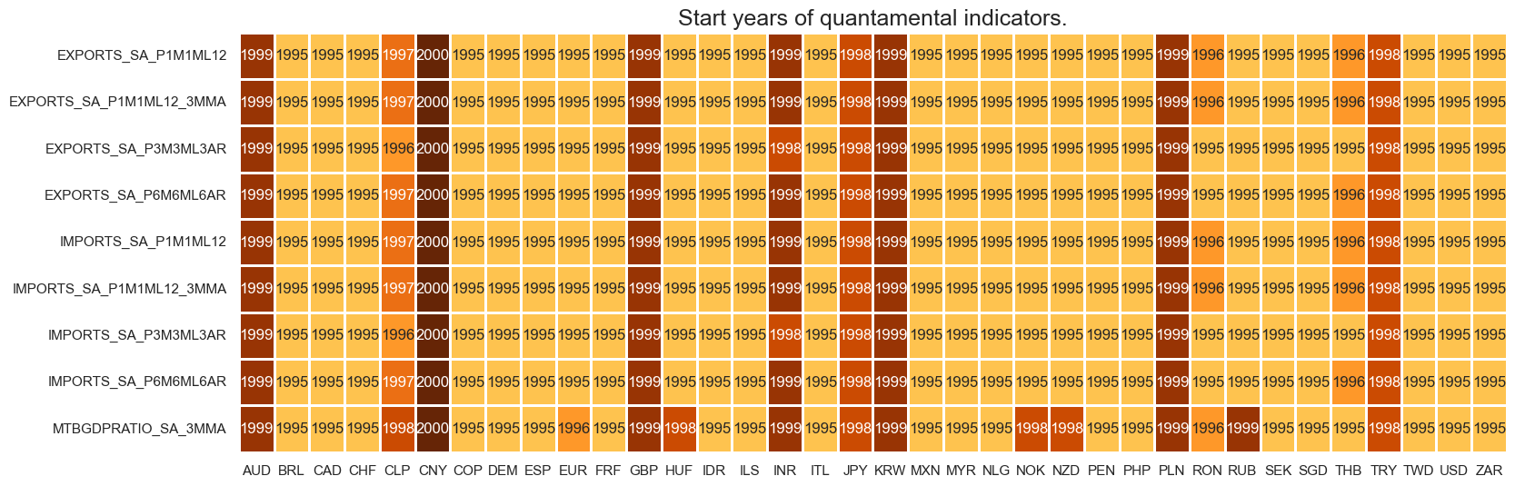
Real-time quantamental indicators of foreign trade trends are available by the mid-1990s for most developed countries and many emerging economies. Some countries’ indicators start only in the early 2000s.

For the explanation of currency symbols, which are related to currency areas or countries for which categories are available, please view Appendix 2 .

             xcatx = main
cidx = cids_exp

dfx = msm.reduce_df(dfd, xcats=xcatx, cids=cidx)
dfs = msm.check_startyears(dfx)
msm.visual_paneldates(dfs, size=(18, 6))

print("Last updated:", date.today())

            

https://macrosynergy.com/notebooks.build/themes/economic-trends/_images/e8700da1455a718b999b7add6f12bce7954d781b8d2664784098c8a49aa94117.png

Last updated: 2024-02-23

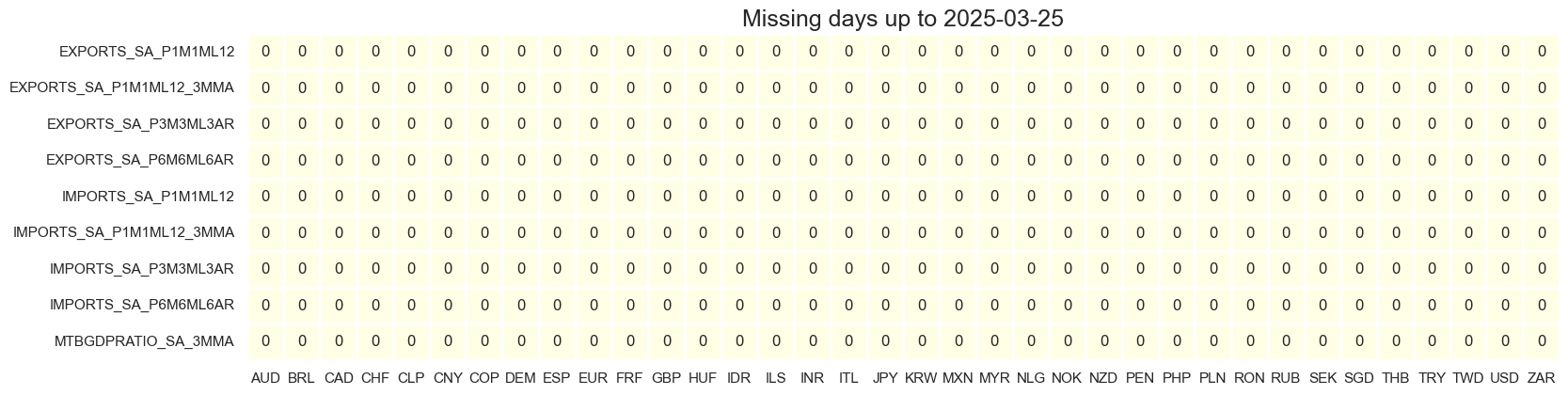
             xcatx = main
cidx = cids_exp

plot = msm.check_availability(
    dfd,
    xcats=xcatx,
    cids=cidx,
    start_size=(18, 6),
    start_years=False,
)

            

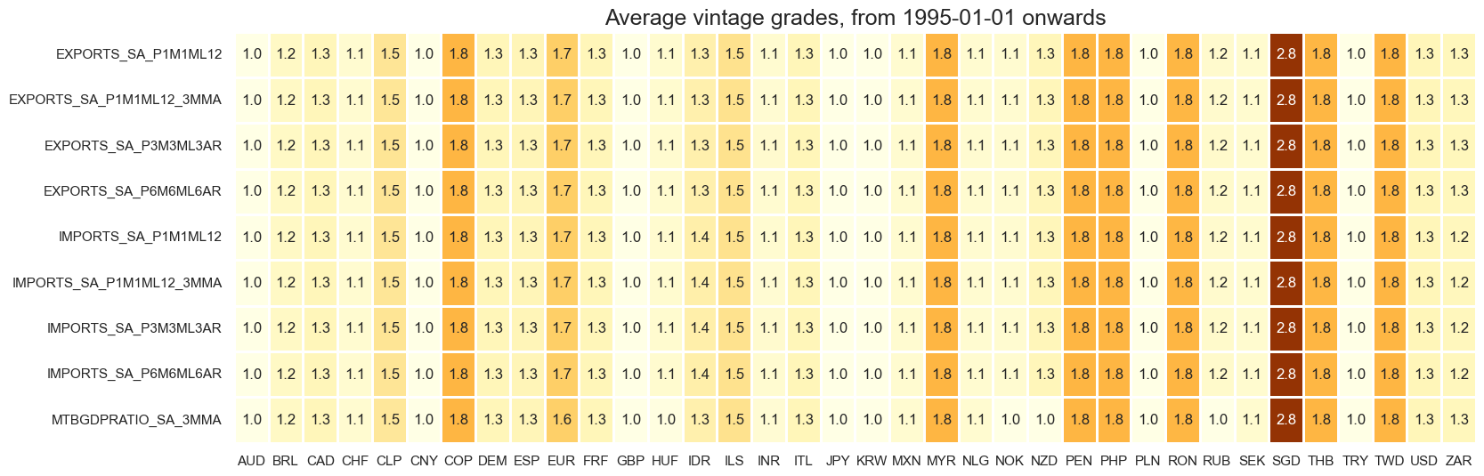
https://macrosynergy.com/notebooks.build/themes/economic-trends/_images/6b919ef47090c7e43a5bae65a341d8dbe70824debb4e7d5db3a10c346f2f7253.png

Vintages are consistently high-graded, with Singapore the notable exception.

             xcatx = main
cidx = cids_exp

plot = msp.heatmap_grades(
    dfd,
    xcats=xcatx,
    cids=cidx,
    start=start_date,
    size=(18, 6),
    title=f"Average vintage grades, from {start_date} onwards",
)

            

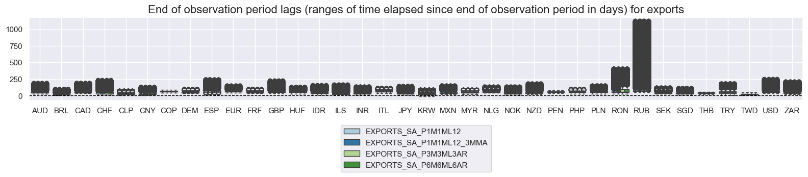
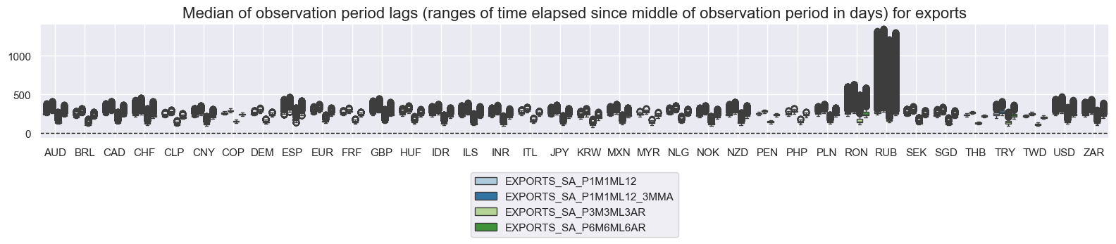
https://macrosynergy.com/notebooks.build/themes/economic-trends/_images/1d70d4b9cd4a0026bb1953318b2298630c6d4cc038a596f38b4abaa4c60308c1.png

             xcatx = [s for s in main if s.startswith("EXPORTS")]
cidx = cids_exp

msp.view_ranges(
    dfd,
    xcats=xcatx,
    cids=cidx,
    val="eop_lag",
    title="End of observation period lags (ranges of time elapsed since end of observation period in days) for exports",
    start=start_date,
    kind="box",
    size=(16, 4),
)
msp.view_ranges(
    dfd,
    xcats=xcatx,
    cids=cidx,
    val="mop_lag",
    title="Median of observation period lags (ranges of time elapsed since middle of observation period in days) for exports",
    start=start_date,
    kind="box",
    size=(16, 4),
)

            

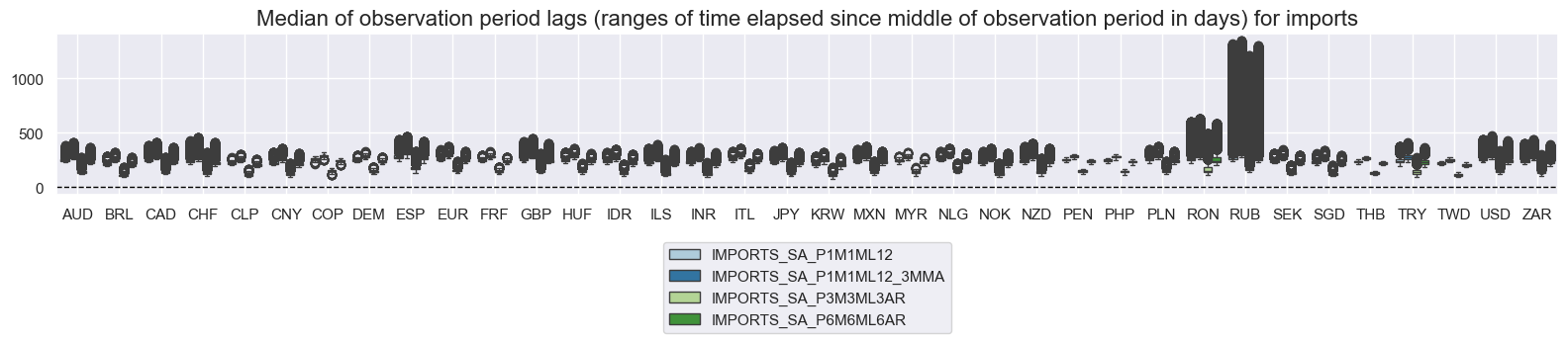
https://macrosynergy.com/notebooks.build/themes/economic-trends/_images/75d0e041ac90faf901d7095fdd89db071ed7c0e6bc0282cbdf52046ea650b6c0.png

https://macrosynergy.com/notebooks.build/themes/economic-trends/_images/6877c300b413019cc49dbe6d7ff1a8a45ede5c0ce100d95cbe95c4b436cab002.png

             xcatx = [s for s in main if s.startswith("IMPORTS")]
cidx = cids_exp

msp.view_ranges(
    dfd,
    xcats=xcatx,
    cids=cidx,
    val="eop_lag",
    title="End of observation period lags (ranges of time elapsed since end of observation period in days) for imports",
    start=start_date,
    kind="box",
    size=(16, 4),
)
msp.view_ranges(
    dfd,
    xcats=xcatx,
    cids=cidx,
    val="mop_lag",
    title="Median of observation period lags (ranges of time elapsed since middle of observation period in days) for imports",
    start=start_date,
    kind="box",
    size=(16, 4),
)

            

https://macrosynergy.com/notebooks.build/themes/economic-trends/_images/b8947451569171a3785273654a7d732f7569f7f1f810ecba072a8b6fb2bdcd00.png

https://macrosynergy.com/notebooks.build/themes/economic-trends/_images/060379d716584c2c00451dc225463bab3eef58d994337a7c5a55ea31361c2356.png

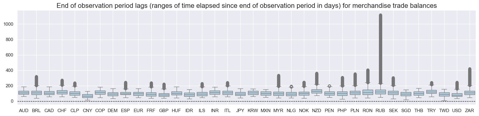
             xcatx = [s for s in main if s.startswith("MTB")]
cidx = cids_exp

msp.view_ranges(
    dfd,
    xcats=xcatx,
    cids=cidx,
    val="eop_lag",
    title="End of observation period lags (ranges of time elapsed since end of observation period in days) for merchandise trade balances",
    start=start_date,
    kind="box",
    size=(16, 4),
)
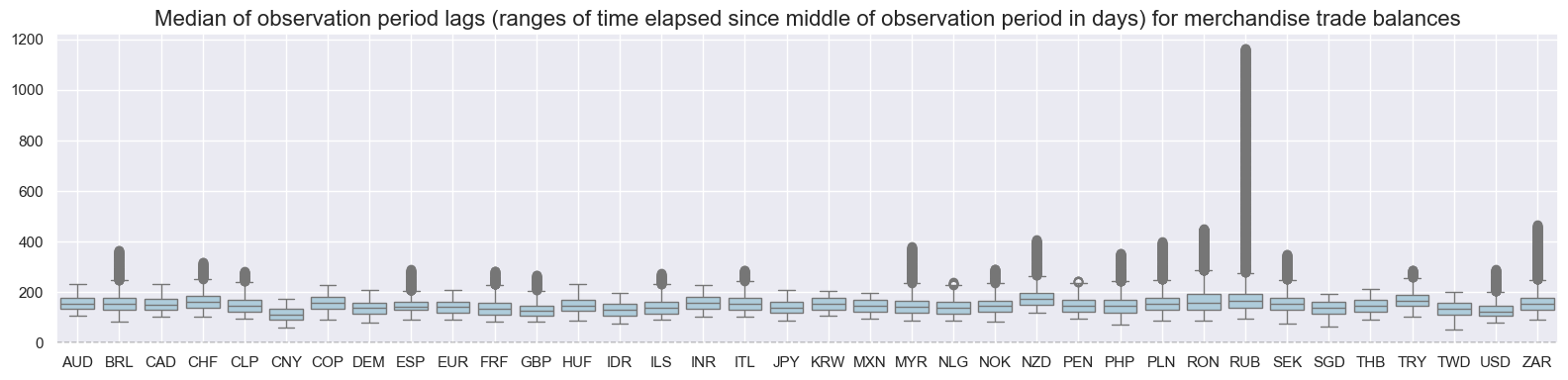
msp.view_ranges(
    dfd,
    xcats=xcatx,
    cids=cidx,
    val="mop_lag",
    title="Median of observation period lags (ranges of time elapsed since middle of observation period in days) for merchandise trade balances",
    start=start_date,
    kind="box",
    size=(16, 4),
)

            

https://macrosynergy.com/notebooks.build/themes/economic-trends/_images/f882c48963798c7cb053d23176d6f20423290bcd2b2a96beaed479bb8b010ccb.png

https://macrosynergy.com/notebooks.build/themes/economic-trends/_images/270603e90b2f52298396760140a7cc17b0fa647bbc688f6152be10c0e59c22a2.png

History #

Annual export growth #

Average annual export growth has ranged from less than 5% (for a range of developed markets) to near 40% (for some emerging economies) since 1995. Since the growth rate is recorded in local currency, high-inflation countries tend to record higher long-term average growth rates.

              xcatx = ["EXPORTS_SA_P1M1ML12", "EXPORTS_SA_P1M1ML12_3MMA"]
cidx = cids_exp
start_date = "1995-01-01"

msp.view_ranges(
    dfd,
    xcats=xcatx,
    cids=cidx,
    sort_cids_by="mean",
    start="1995-01-01",
    title="Means and standard deviations of annual merchandise export trends since 1995",
    xcat_labels=[
        "% over a year ago, seasonally-adjusted",
        "3-month moving average, % over a year ago, seasonally-adjusted",
    ],
    kind="bar",
    size=(16, 8),
)

             

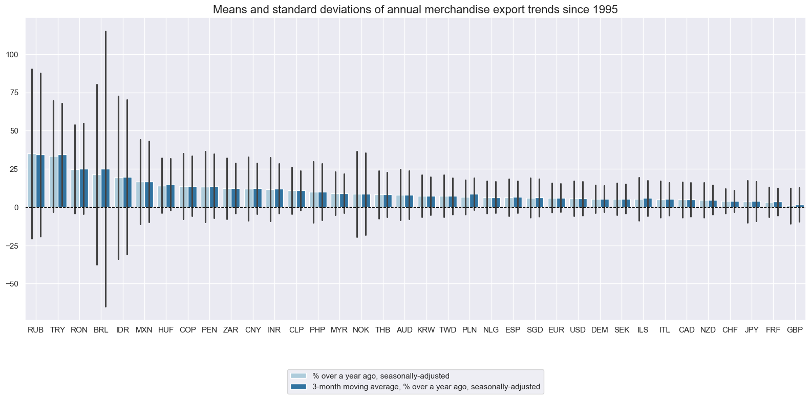
https://macrosynergy.com/notebooks.build/themes/economic-trends/_images/db46e0d55df4273ccb03c752ff8ab8db90d98d976159695751ef2d21710d4439.png

Periods of very high local-currency export growth have often been associated with currency depreciation, such as in Brazil and Indonesia in the 1990s.

              xcatx = ["EXPORTS_SA_P1M1ML12", "EXPORTS_SA_P1M1ML12_3MMA"]
cidx = cids_exp
start_date = "1995-01-01"

msp.view_timelines(
    dfd,
    xcats=xcatx,
    cids=cidx,
    start=start_date,
    title="Exports growth, seasonally-adjusted, % over a year ago and 3-month moving average thereof",
    title_fontsize=27,
    legend_fontsize=17,
    label_adj=0.075,
    xcat_labels=["% over a year ago", "3-month moving average, % over a year ago"],
    ncol=4,
    same_y=False,
    size=(12, 7),
    aspect=1.7,
    all_xticks=True,
)

             

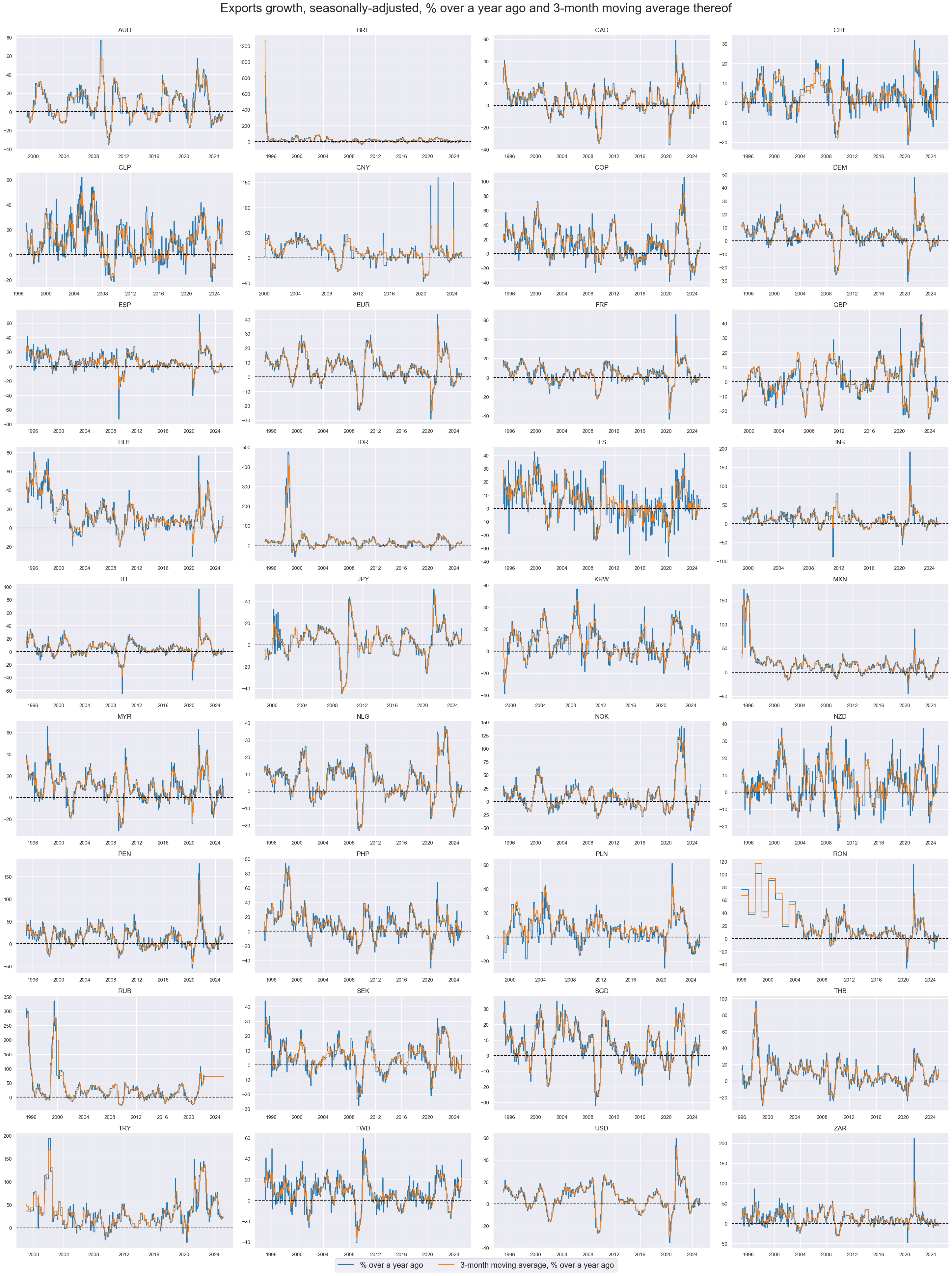
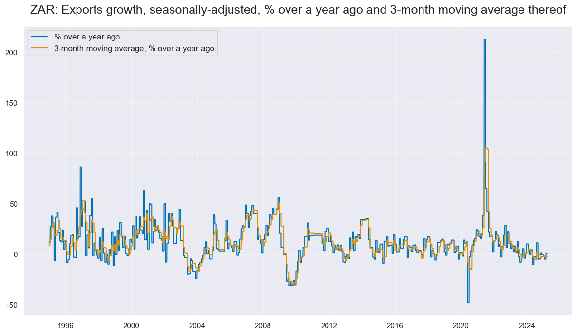
https://macrosynergy.com/notebooks.build/themes/economic-trends/_images/a55c249dff1ee83c1bb7ae93a54d8d5ee4fe4ded41aceffe894516407ac63128.png

For many countries, the disruptions caused by the COVID-19 pandemic led to unprecedented outliers in 2020/21, with asymmetric effects on the growth rates, because rebounds were calculated based on an extraordinarily low base.

              xcatx = ["EXPORTS_SA_P1M1ML12", "EXPORTS_SA_P1M1ML12_3MMA"]
cidx = ["ZAR"]
start_date = "1995-01-01"

msp.view_timelines(
    dfd,
    xcats=xcatx,
    cids=cidx,
    start=start_date,
    title=f"{cidx[0]}: Exports growth, seasonally-adjusted, % over a year ago and 3-month moving average thereof",
    title_adj=1.03,
    xcat_labels=["% over a year ago", "3-month moving average, % over a year ago"],
    size=(12, 7),
    aspect=1.7,
)

             

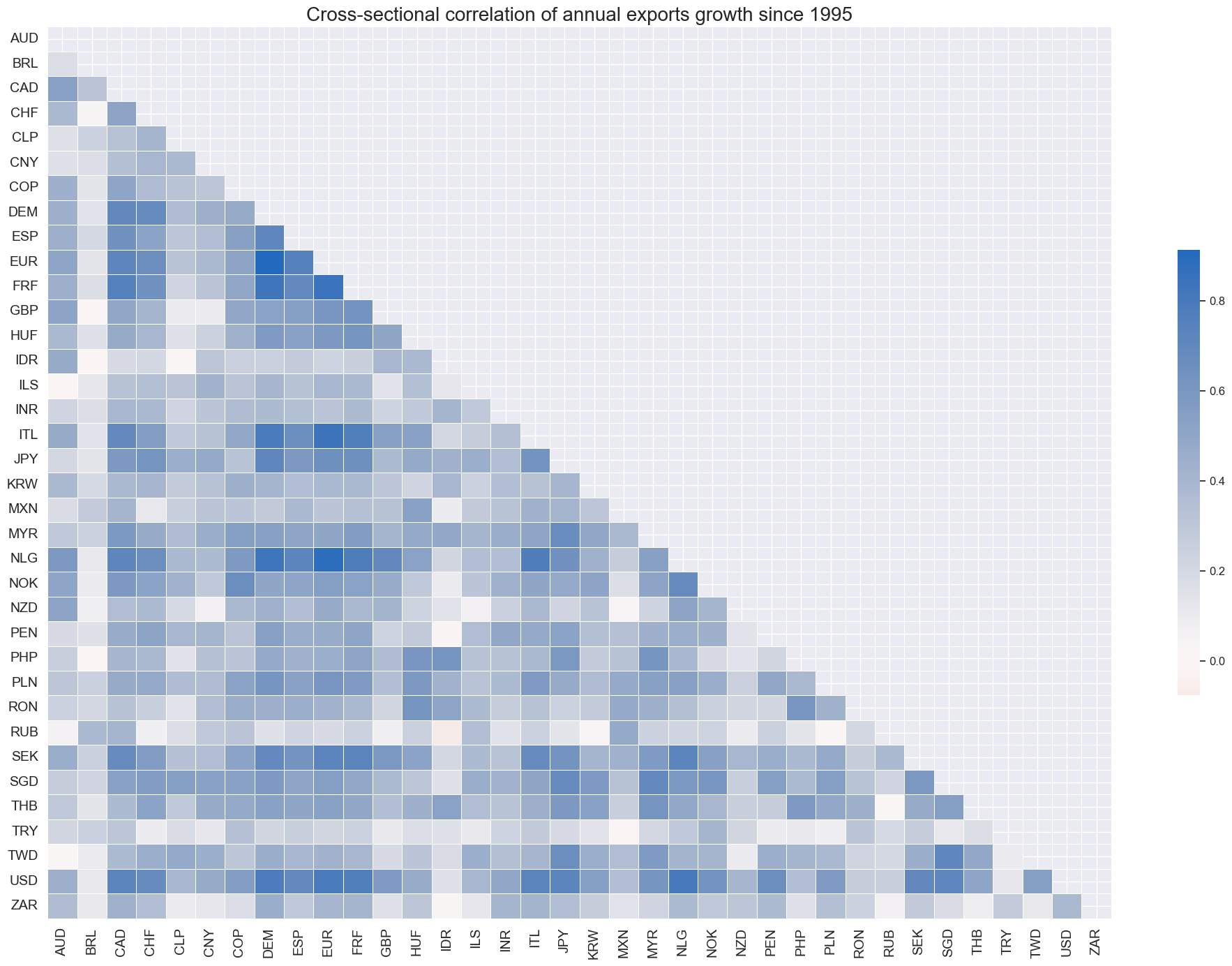
https://macrosynergy.com/notebooks.build/themes/economic-trends/_images/2995282f39b8b515f4ed2bce61c9089e8e20616dc37f0963050c9c56e577388a.png

The real-time indicators of annual export growth have been positively correlated across almost all country pairs.

              xcatx = ["EXPORTS_SA_P1M1ML12"]
cidx = cids_exp
start_date = "1995-01-01"

msp.correl_matrix(
    dfd,
    xcats=xcatx,
    cids=cidx,
    size=(20, 14),
    start=start_date,
    title="Cross-sectional correlation of annual exports growth since 1995",
)

             

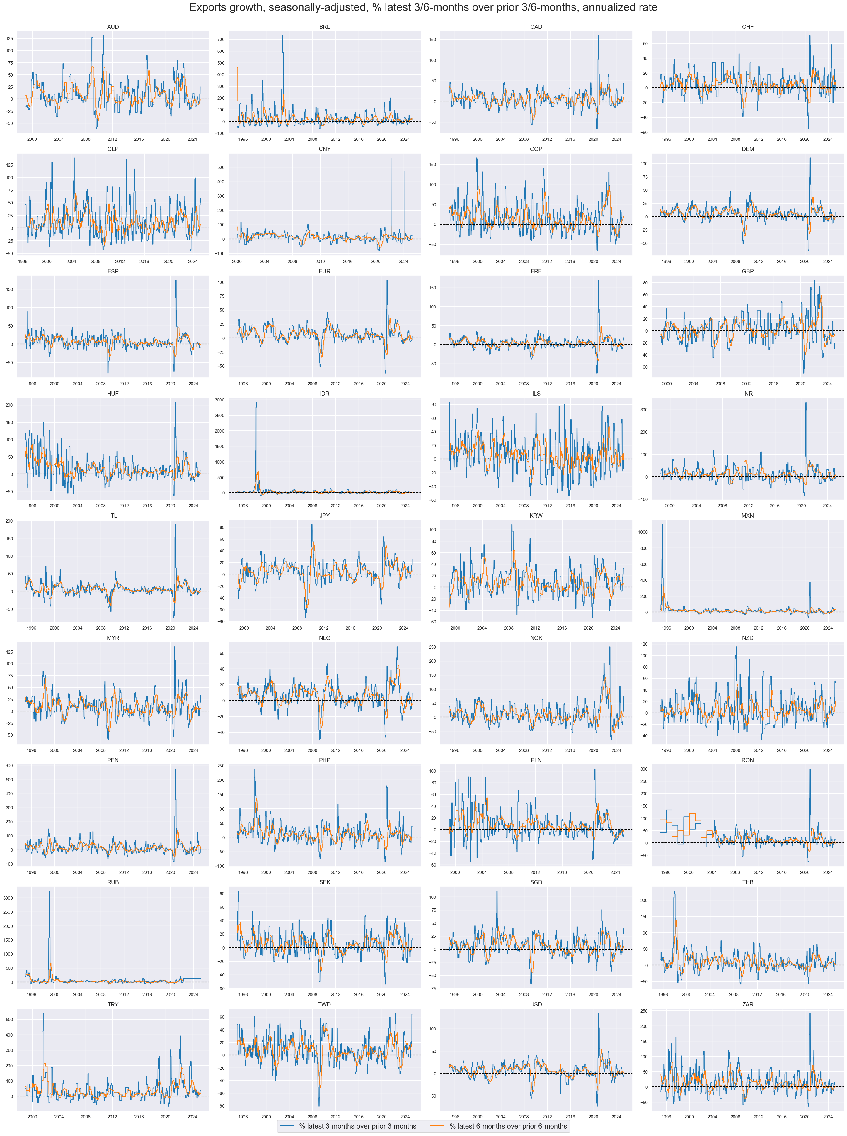
https://macrosynergy.com/notebooks.build/themes/economic-trends/_images/7ae6a1044ab44a87c91becab9c15c4f8c084f10f7291e4fced8f0f3fa2ddeb09.png

Short-term export trends #

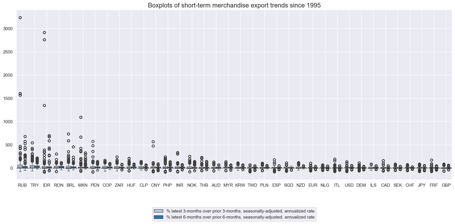
EM countries have on average recorded higher volatility in short-term export trends. High-inflation and currency instability in the 1990s as well as the COVID pandemic have produced extreme outliers in short-term export trends for some countries.

              xcatx = ["EXPORTS_SA_P3M3ML3AR", "EXPORTS_SA_P6M6ML6AR"]
cidx = cids_exp
start_date = "1995-01-01"

msp.view_ranges(
    dfd,
    xcats=xcatx,
    cids=cidx,
    sort_cids_by="mean",
    start=start_date,
    kind="box",
    size=(16, 8),
    title="Boxplots of short-term merchandise export trends since 1995",
    xcat_labels=[
        "% latest 3-months over prior 3-months, seasonally-adjusted, annualized rate",
        "% latest 6-months over prior 6-months, seasonally-adjusted, annualized rate",
    ],
)

             

https://macrosynergy.com/notebooks.build/themes/economic-trends/_images/c53eca0cfd2db9ca56d37b2f45d3407e3cd4aea2c258c97fea790fb1d17ce93c.png

              xcatx = ["EXPORTS_SA_P3M3ML3AR", "EXPORTS_SA_P6M6ML6AR"]
cidx = cids_exp
start_date = "1995-01-01"

msp.view_timelines(
    dfd,
    xcats=xcatx,
    cids=cidx,
    start=start_date,
    title="Exports growth, seasonally-adjusted, % latest 3/6-months over prior 3/6-months, annualized rate",
    label_adj=0.075,
    title_fontsize=27,
    legend_fontsize=17,
    xcat_labels=[
        "% latest 3-months over prior 3-months",
        "% latest 6-months over prior 6-months",
    ],
    ncol=4,
    same_y=False,
    size=(12, 7),
    aspect=1.7,
    all_xticks=True,
)

             

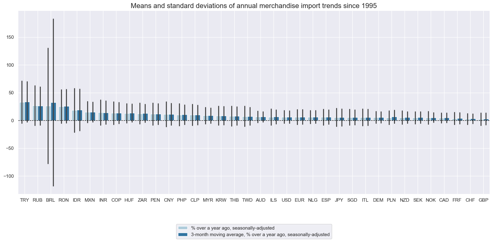
https://macrosynergy.com/notebooks.build/themes/economic-trends/_images/bd13c9f54eba629936efd34b0a2bce9a53ee0e91f6de1945b132dfc6ff10675b.png

Annual import growth #

Long-term average import growth in local currency has naturally been highest in EM and higher-inflation economies. As for exports, the local currency value had a great bearing on import value growth over time and across countries.

              xcatx = ["IMPORTS_SA_P1M1ML12", "IMPORTS_SA_P1M1ML12_3MMA"]
cidx = cids_exp
start_date = "1995-01-01"

msp.view_ranges(
    dfd,
    xcats=xcatx,
    cids=cidx,
    sort_cids_by="mean",
    start=start_date,
    kind="bar",
    size=(16, 8),
    title="Means and standard deviations of annual merchandise import trends since 1995",
    xcat_labels=[
        "% over a year ago, seasonally-adjusted",
        "3-month moving average, % over a year ago, seasonally-adjusted",
    ],
)

             

https://macrosynergy.com/notebooks.build/themes/economic-trends/_images/d6ff1ae214bbcaf9985c6f624d2cf77b47d963dbd6a8dc5f96b2479e3fc53304.png

              xcatx = ["IMPORTS_SA_P1M1ML12", "IMPORTS_SA_P1M1ML12_3MMA"]
cidx = cids_exp
start_date = "1995-01-01"

msp.view_timelines(
    dfd,
    xcats=xcatx,
    cids=cidx,
    start=start_date,
    title="Imports growth, seasonally-adjusted, % over a year ago and 3-month moving average thereof",
    title_fontsize=27,
    legend_fontsize=17,
    label_adj=0.075,
    xcat_labels=["% over a year ago", "3-month moving average, % over a year ago"],
    ncol=4,
    same_y=False,
    size=(12, 7),
    aspect=1.7,
    all_xticks=True,
)

             

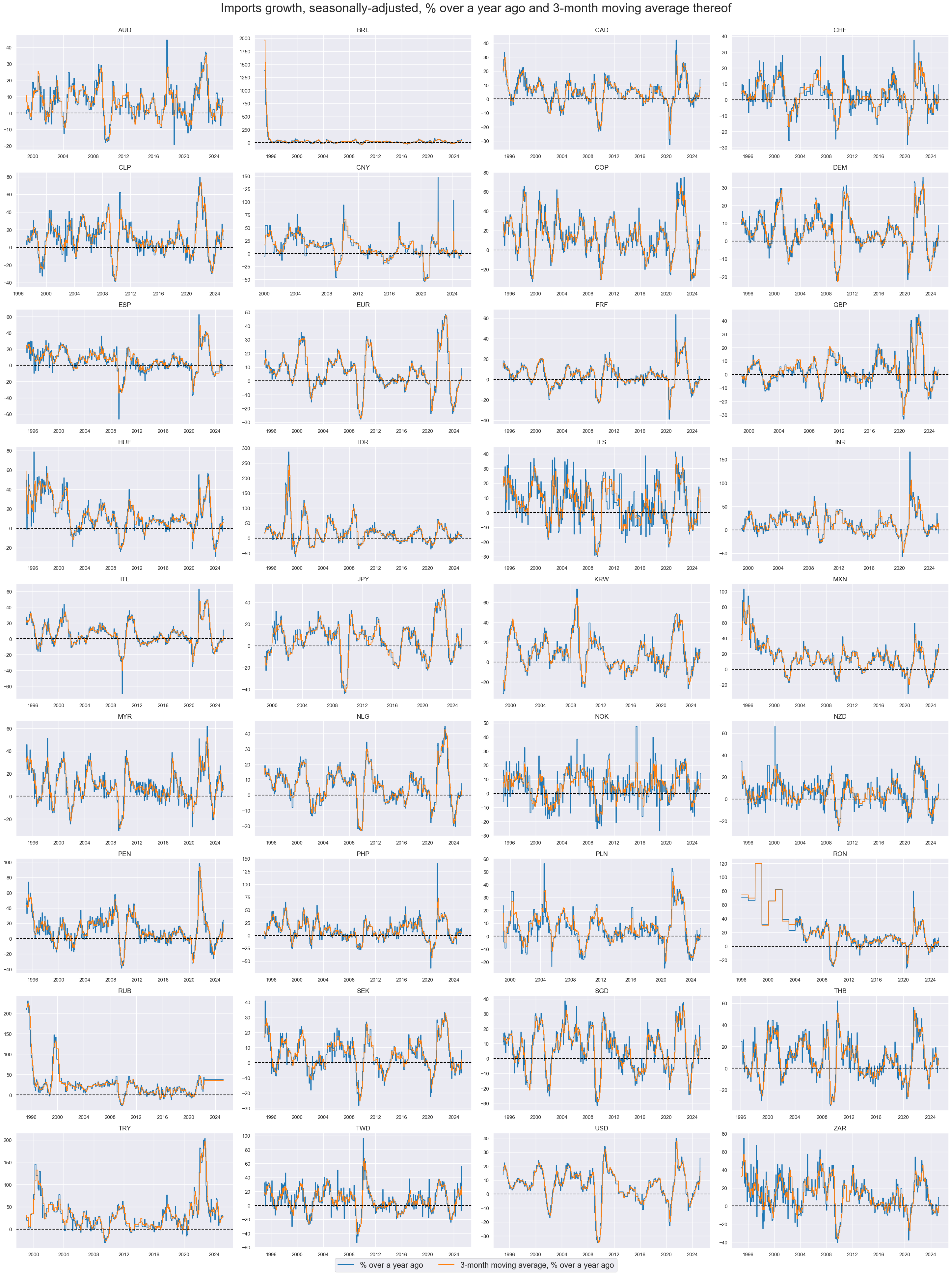
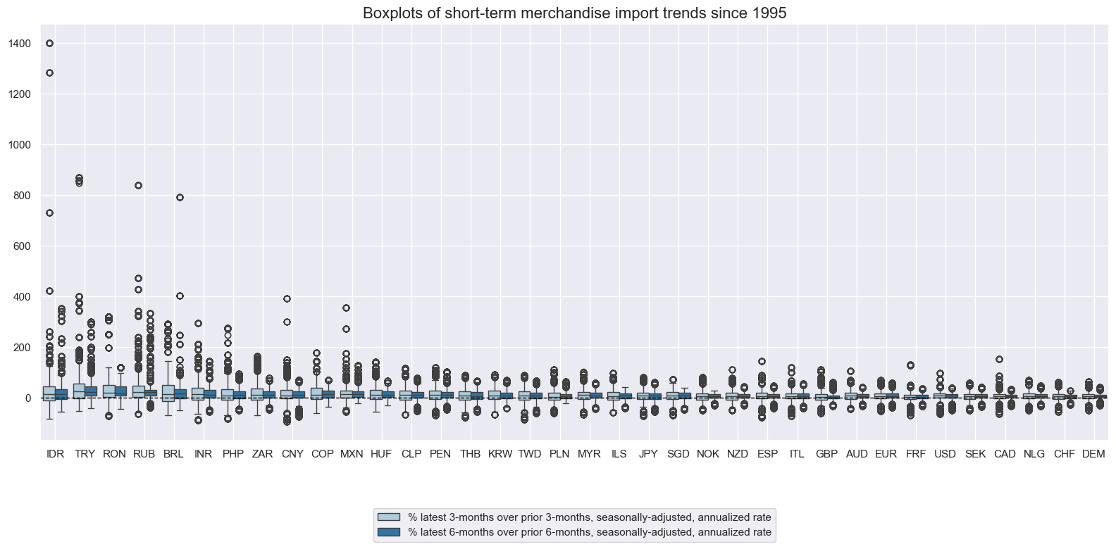
https://macrosynergy.com/notebooks.build/themes/economic-trends/_images/c84b0422b712c71b6caa6094369e7b49ca071192032eee17964c5c9c0f3d9305.png

Short-term merchandise import trends #

Short-term import growth trends have been very volatile and prone to outliers.

              xcatx = ["IMPORTS_SA_P3M3ML3AR", "IMPORTS_SA_P6M6ML6AR"]
cidx = cids_exp
start_date = "1995-01-01"

msp.view_ranges(
    dfd,
    xcats=xcatx,
    cids=cidx,
    sort_cids_by="std",
    start=start_date,
    kind="box",
    size=(16, 8),
    title="Boxplots of short-term merchandise import trends since 1995",
    xcat_labels=[
        "% latest 3-months over prior 3-months, seasonally-adjusted, annualized rate",
        "% latest 6-months over prior 6-months, seasonally-adjusted, annualized rate",
    ],
)

             

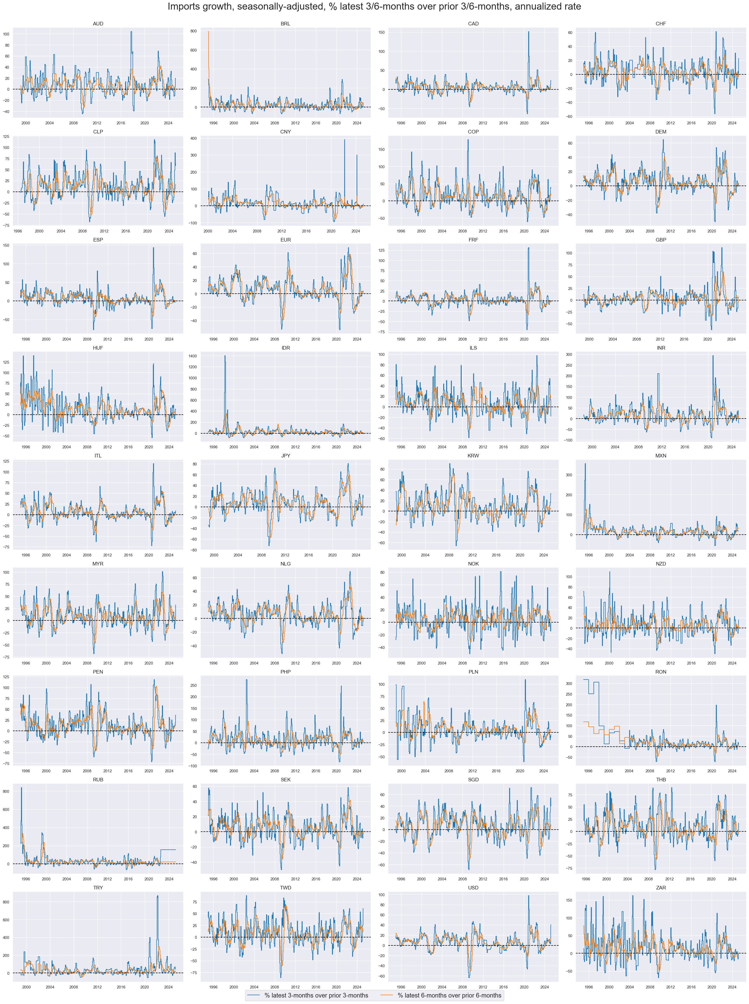
https://macrosynergy.com/notebooks.build/themes/economic-trends/_images/631a2a2107dfaef0b32c15a71b47b890dc171fa654400c92b27c26d2b37efe4f.png

              xcatx = ["IMPORTS_SA_P3M3ML3AR", "IMPORTS_SA_P6M6ML6AR"]
cidx = cids_exp

msp.view_timelines(
    dfd,
    xcats=xcatx,
    cids=cidx,
    start=start_date,
    title="Imports growth, seasonally-adjusted, % latest 3/6-months over prior 3/6-months, annualized rate",
    title_fontsize=27,
    label_adj=0.075,
    legend_fontsize=17,
    xcat_labels=[
        "% latest 3-months over prior 3-months",
        "% latest 6-months over prior 6-months",
    ],
    ncol=4,
    same_y=False,
    size=(15, 7),
    aspect=1.7,
    all_xticks=True,
)

             

https://macrosynergy.com/notebooks.build/themes/economic-trends/_images/331798974201d6e0f5d8f38cdf756b6b8189a596cc776bd23f6cdff75a8655de.png

Importance #

Research links #

“We examine the stability and strength of the relationship between exchange rates and trade over time…We find that trade elasticities are generally stable…We estimate that a 10% effective depreciation in an economy’s currency is associated on average with a 1.5% of GDP increase in net exports.” IMF

Empirical clues #

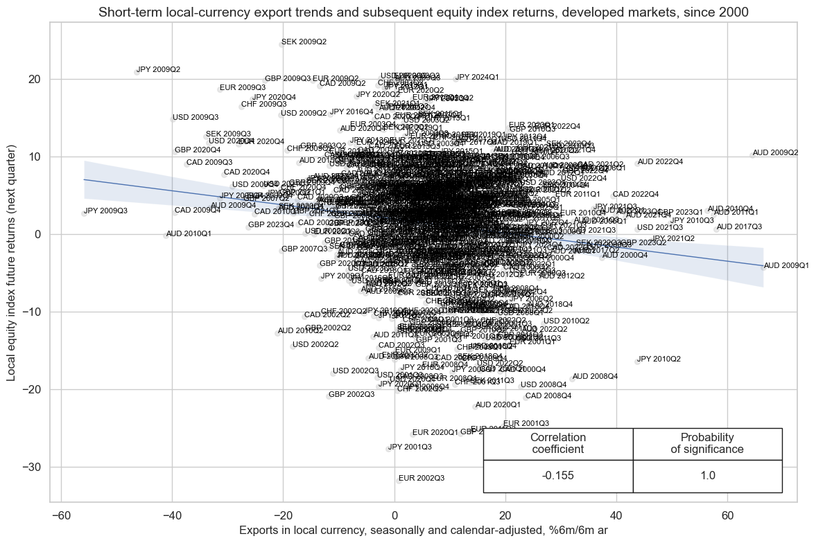
Stronger short-term local currency export trends have on average been associated with lower subsequent local equity index future returns. This may reflect that high export value growth typically bodes for tighter monetary conditions. The relationship is strongest for developed markets.

              xcatx = ["EXPORTS_SA_P6M6ML6AR", "EQXR_NSA"]
cidx = list(set(cids_dm) - set(["DEM", "ESP", "FRF", "ITL", "NLG", "NOK", "NZD"]))
cr = msp.CategoryRelations(
    dfd,
    xcats=xcatx,
    cids=cidx,
    freq="Q",
    lag=1,
    xcat_aggs=["last", "sum"],
    start="2000-01-01",
)

cr.reg_scatter(
    title="Short-term local-currency export trends and subsequent equity index returns, developed markets, since 2000",
    labels=True,
    coef_box="lower right",
    xlab="Exports in local currency, seasonally and calendar-adjusted, %6m/6m ar",
    ylab="Local equity index future returns (next quarter)",
    reg_robust=False,
)

             

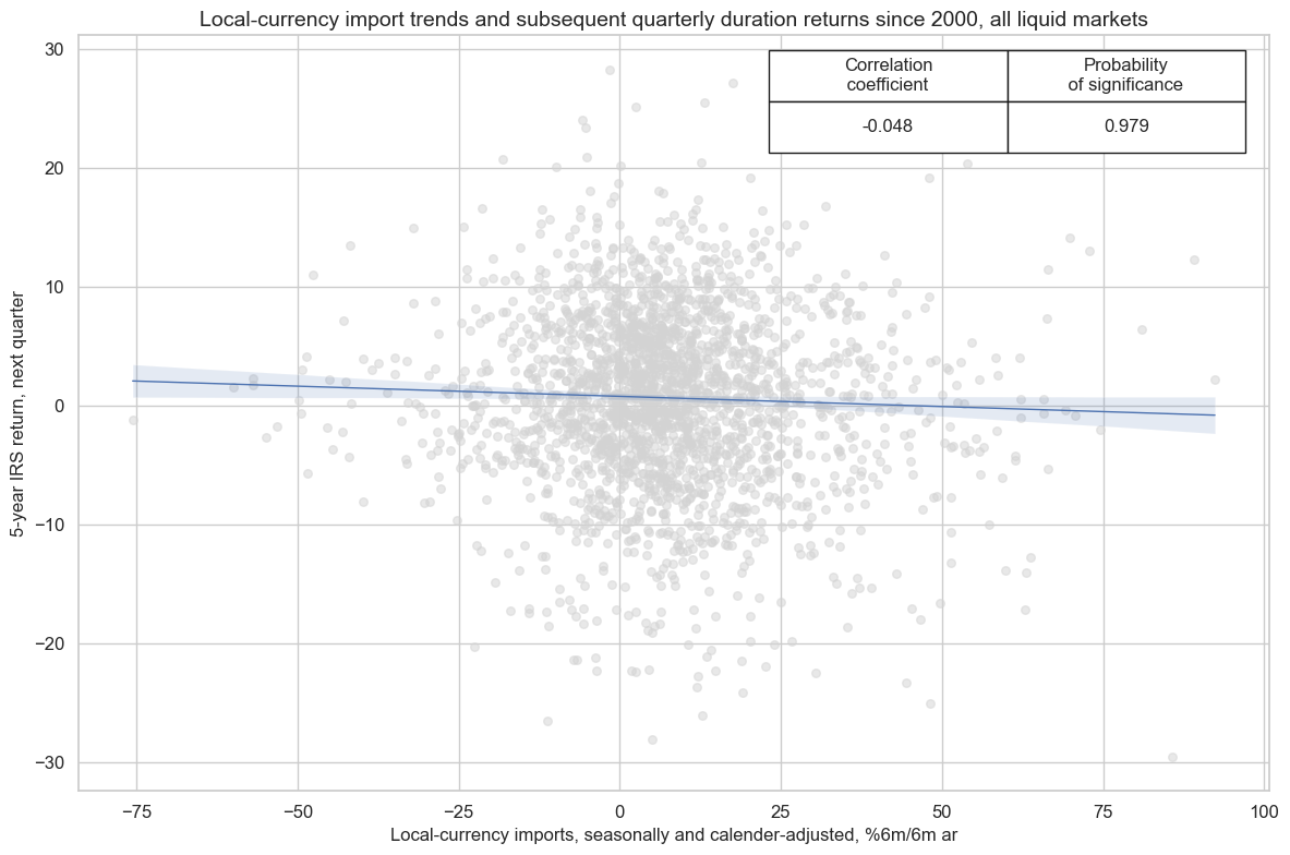
https://macrosynergy.com/notebooks.build/themes/economic-trends/_images/b98d179e8f7d8684fbdb34a0e04f146c432a81770152e2b254d2e1461fd6cf45.png

Strong short-term import trends, which are indicative of stronger nominal local demand, have on average been associated with weaker subsequent duration returns.

              xcatx = ["IMPORTS_SA_P6M6ML6AR", "DU05YXR_VT10"]
cidx = cids

cr = msp.CategoryRelations(
    dfd,
    xcats=xcatx,
    cids=list(
        set(cidx)
        - set(["BRL", "DEM", "ESP", "FRF", "HKD", "ITL", "NLG", "PEN", "PHP", "RON"])
    ),
    freq="Q",
    lag=1,
    xcat_aggs=["last", "sum"],
    fwin=1,
    start="2000-01-01",
    xcat_trims=[100, 30],
)

cr.reg_scatter(
    title="Local-currency import trends and subsequent quarterly duration returns since 2000, all liquid markets",
    labels=False,
    coef_box="upper right",
    xlab="Local-currency imports, seasonally and calender-adjusted, %6m/6m ar",
    ylab="5-year IRS return, next quarter",
    reg_robust=True,
)

             

https://macrosynergy.com/notebooks.build/themes/economic-trends/_images/ee8c465d30c0de2cf463b42a96504e1a6d2bc4857b678d35a228227f45484940.png

Appendices #

Appendix 1: Notes on OECD data integration #

National sources series’ used to construct indicators in this category group are complemented by vintages provided by OECD’s ‘Revision Analysis’ dataset. The integration of the OECD datasets follows the following rules:

The following priority order is applied for combining vintages. First, JPMaQS uses seasonally and calendar adjusted original vintages from national sources. Beyond that JPMaQS uses OECD vintages.
OECD vintages inform on the month of release but not the exact date. Actual release dates for these vintages are estimated based on release days of subsequent vintages.
Inconsistencies, data errors and missing values in the OECD vintages have been corrected for JPMaQS.

OECD data is seasonally adjusted and denominated in native currency. No such consistency is found in national sources. Often figures are stated in a foreign denomination (EUR or USD) and no seasonal adjustment has been applied. To integrate these two data sources we first currency convert national sources into their native currency and then apply seasonal adjustment.

Appendix 2: Currency symbols #

The word ‘cross-section’ refers to currencies, currency areas or economic areas. In alphabetical order, these are AUD (Australian dollar), BRL (Brazilian real), CAD (Canadian dollar), CHF (Swiss franc), CLP (Chilean peso), CNY (Chinese yuan renminbi), COP (Colombian peso), CZK (Czech Republic koruna), DEM (German mark), ESP (Spanish peseta), EUR (Euro), FRF (French franc), GBP (British pound), HKD (Hong Kong dollar), HUF (Hungarian forint), IDR (Indonesian rupiah), ITL (Italian lira), JPY (Japanese yen), KRW (Korean won), MXN (Mexican peso), MYR (Malaysian ringgit), NLG (Dutch guilder), NOK (Norwegian krone), NZD (New Zealand dollar), PEN (Peruvian sol), PHP (Phillipine peso), PLN (Polish zloty), RON (Romanian leu), RUB (Russian ruble), SEK (Swedish krona), SGD (Singaporean dollar), THB (Thai baht), TRY (Turkish lira), TWD (Taiwanese dollar), USD (U.S. dollar), ZAR (South African rand).