Emerging markets bond index returns #
The category group features daily generic returns of two major emerging market indices, the JP Morgan Government Bond Index in local currency, and the EMBI Global (EMBIG), in hard currency.
Local currency bond index returns #
Ticker : LCBIR_NSA / LCBIXR_NSA / LCBIXR_VT10
Label : Local currency bond index (GBI-EM): cash returns / excess returns / excess returns for 10% vol target
Definition : Local currency bond index (J.P. Morgan GBI-EM): cash returns / excess returns / excess returns for 10% vol target
Notes :
-
The J.P. Morgan Government Bond Index Emerging Markets (GBI-EM) provides investors with a benchmark that tracks local currency bonds issued by emerging market governments. The GBI-EM closely follows the methodology of JPM’s family of GBI Indices, which are widely used as benchmarks for investing in developed government bond markets. More information on index specifications is presented in Appendix 1 .
-
The level of the index is a synthetic value calculated from the weighted average of returns of the bonds in the index. The underlying calculations are explained in Appendix 2 .
-
Excess returns are calculated utilising local short term interest rates. For most countries, a 1-month Libor rate has historically been used as a proxy for local funding costs. However, in the wake of the benchmark rate reform, this changed to other rates. For more information on the specific short term nominal interest rates used, please see here .
-
For excess return calculation the risk-free rate is “de-annualized” by dividing by 252 business days, so that it is in line with our daily return calculation. For a detailed explanation of the excess return calculation also see Appendix 2
-
For more information on the GBI-EM methodology, see here
Foreign currency bond index returns #
Ticker : FCBIR_NSA / FCBIXR_NSA / FCBIXR_VT10
Label : Foreign currency bond index (EMBIG): cash returns / excess returns / excess returns for 10% vol target
Definition : Foreign currency bond index (J.P. Morgan EMBIG): cash returns / excess returns / excess returns for 10% vol target
Notes :
-
The EMBI Global (EMBIG) includes USD-denominated bonds from EM sovereign & quasi-sovereign issuers. The EMBI suite of indices considers US dollar-denominated bonds issued by sovereign and quasi-sovereign EM entities eligible for inclusion. More information on index specifications is presented in Appendix 1 .
-
The level of the index is a synthetic value calculated from the weighted average of returns of the bonds in the index. The underlying calculations are explained in Appendix 2 .
-
For Chile and Egypt we use a different index definition (aggregate traded index), due to that type’s longer availability.
-
For volatility targeting positions are scaled to 10% vol target based on historic standard deviation for an exponential moving average with a half- time of 11 days. Positions are rebalanced at the end of each month.
-
Excess returns are calculated utilising USD short term interest rates. For excess return calculation the risk-free rate is “de-annualized” by dividing by 252 business days, so that it is in line with our daily return calculation. For a detailed explanation of the excess return calculation also see Appendix 2
Local currency bond index returns in USD #
Ticker : LCBIRUSD_NSA / LCBIXRUSD_NSA / LCBIXRUSD_VT10
Label : Local currency bond index (GBI-EM) converted into USD: cash returns in USD / excess returns in USD / excess returns in USD for 10% vol target
Definition : Local currency bond index (J.P. Morgan GBI-EM) in USD: cash returns in USD / excess returns in USD / excess returns in USD for 10% vol target
Notes :
-
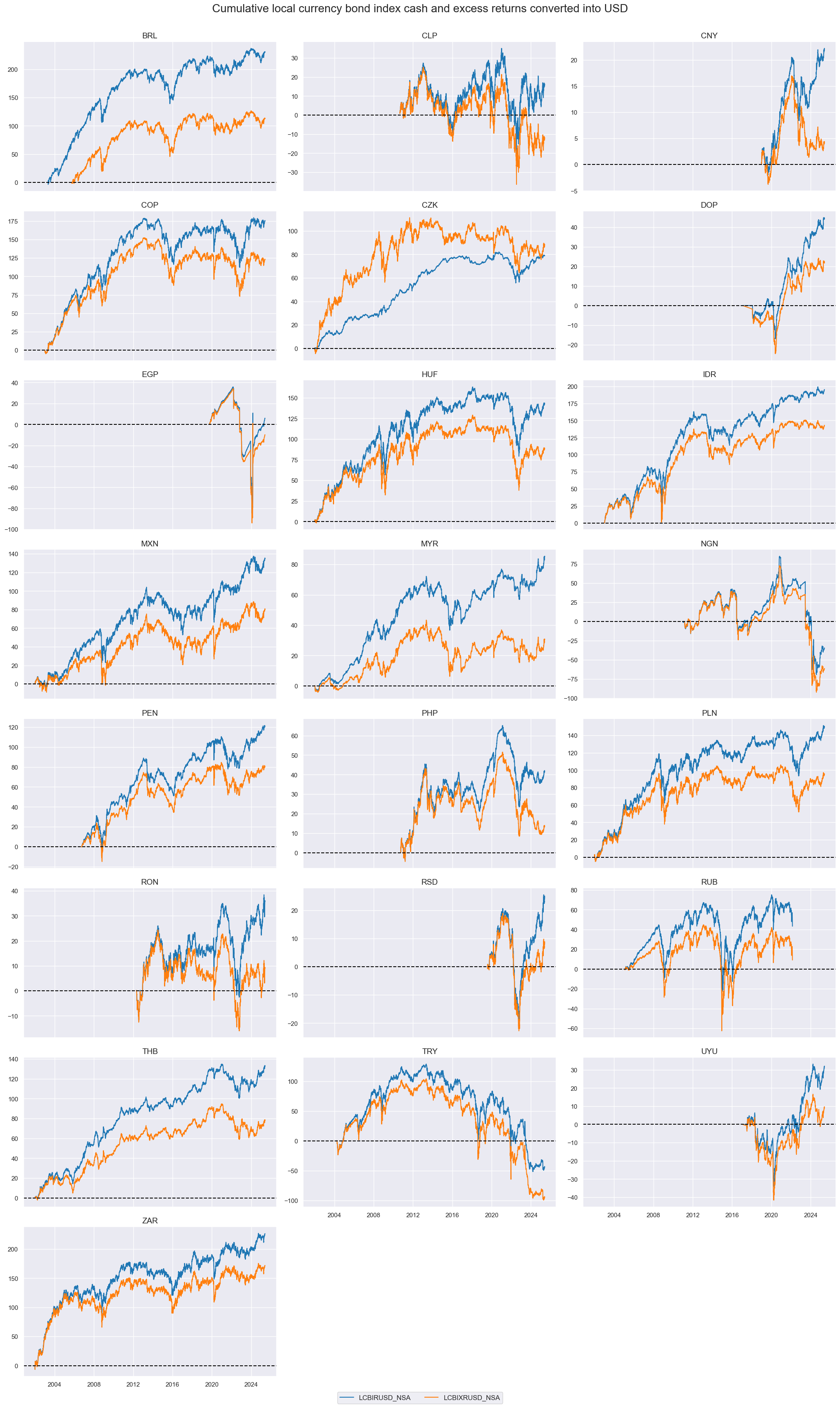
These returns come from the above J.P. Morgan Government Bond Dollar Index (GBI-EM in dollars). The level of the index is a synthetic value calculated from the weighted average of USD returns of the bonds in the index. The returns are converted into US dollars daily according to the WMR 4PM London level. These returns provide a comparable representation for USD-based investors looking to invest in local currency bonds and to convert their holdings back into hard currency.
-
The nominal interest rate used for excess returns is the USD nominal rate. For more information on the specific short term nominal interest rates used, please see here .
-
For excess return calculation the risk-free rate is “de-annualized” by dividing by 252 business days, so that it is in line with our daily return calculation. For a detailed explanation of the excess return calculation also see Appendix 2
-
For Egypt, in December 2023, the 12 month NDF rate captured by WMR starts being used in order to reflect ‘mark-to-market’ fx losses. In January 2024, Egypt was removed from the GBI-EM indices - and in March, the index goes back to using the standalone FX spot rate.
Imports #
Only the standard Python data science packages and the specialized
macrosynergy
package are needed.
import os
import numpy as np
import pandas as pd
import matplotlib.pyplot as plt
import seaborn as sns
import math

import json
import yaml

import macrosynergy.management as msm
import macrosynergy.panel as msp
import macrosynergy.signal as mss
import macrosynergy.pnl as msn


from macrosynergy.download import JPMaQSDownload

from timeit import default_timer as timer
from datetime import timedelta, date, datetime

import warnings

warnings.simplefilter("ignore")
The
JPMaQS
indicators we consider are downloaded using the J.P. Morgan Dataquery API interface within the
macrosynergy
package. This is done by specifying
ticker strings
, formed by appending an indicator category code
<category>
to a currency area code
<cross_section>
. These constitute the main part of a full quantamental indicator ticker, taking the form
DB(JPMAQS,<cross_section>_<category>,<info>)
, where
<info>
denotes the time series of information for the given cross-section and category. The following types of information are available:
-
valuegiving the latest available values for the indicator -
eop_lagreferring to days elapsed since the end of the observation period -
mop_lagreferring to the number of days elapsed since the mean observation period -
gradedenoting a grade of the observation, giving a metric of real time information quality.
After instantiating the
JPMaQSDownload
class within the
macrosynergy.download
module, one can use the
download(tickers,start_date,metrics)
method to easily download the necessary data, where
tickers
is an array of ticker strings,
start_date
is the first collection date to be considered and
metrics
is an array comprising the times series information to be downloaded.
Currency areas are identified by currency symbols as explained in Appendix 3 .
cids_lc_latam = [  # Latam local currency debt countries
    "BRL",
    "CLP",
    "COP",
    "DOP",
    "MXN",
    "PEN",
    "UYU",
]
cids_lc_emeu = [  # EM Europe local currency debt countries
    "CZK",
    "HUF",
    "PLN",
    "RON",
    "RUB",
    "RSD",
    "TRY",
]
cids_lc_meaf = [  # Middle-East and Africa local currency debt countries
    "EGP",
    "NGN",
    "ZAR",
]
cids_lc_asia = [  # Asia local currency debt countries
    "CNY",
    "IDR",
    "MYR",
    "PHP",
    "THB",
]

cids_lc = sorted(list(set(cids_lc_latam + cids_lc_emeu + cids_lc_meaf + cids_lc_asia)))


cids_fc_latam = [  # Latam foreign currency debt countries
    "BRL",
    "CLP",
    "COP",
    "DOP",
    "MXN",
    "PEN",
    "UYU",
]
cids_fc_emeu = [  # EM Europe foreign currency debt countries
    "HUF",
    "PLN",
    "RON",
    "RUB",
    "RSD",
    "TRY",
]
cids_fc_meaf = [  # Middle-East and Africa foreign currency debt countries
    "AED",
    "BHD",
    "EGP",
    "NGN",
    "OMR",
    "QAR",
    "ZAR",
]
cids_fc_asia = [  # Asia foreign currency debt countries
    "CNY",
    "IDR",
    "INR",
    "PHP",
    "SAR",
]
cids_fc = sorted(list(set(cids_fc_latam + cids_fc_emeu + cids_fc_meaf + cids_fc_asia)))
cids = sorted(list(set(cids_lc + cids_fc)))
locs = [
    "LCBIR_NSA",
    "LCBIXR_NSA",
    "LCBIXR_VT10",
]

locs_usd = [
    "LCBIRUSD_NSA",
    "LCBIXRUSD_NSA",
    "LCBIXRUSD_VT10",
]

fors = [
    "FCBIR_NSA",
    "FCBIXR_NSA",
    "FCBIXR_VT10",
]
main = locs + fors

xtra = [
    "REER_NSA_P1W4WL1",
    "REER_NSA_P1M1ML12",
    "REER_NSA_P1M60ML1",
    "REEROADJ_NSA_P1W4WL1",
    "REEROADJ_NSA_P1M1ML12",
    "REEROADJ_NSA_P1M60ML1",
]

xcats = main + xtra + locs_usd
# Download series from J.P. Morgan DataQuery by tickers

start_date = "2002-01-01"
tickers = [cid + "_" + xcat for cid in cids for xcat in xcats]
print(f"Maximum number of tickers is {len(tickers)}")

# Retrieve credentials

client_id: str = os.getenv("DQ_CLIENT_ID")
client_secret: str = os.getenv("DQ_CLIENT_SECRET")

# Download from DataQuery

with JPMaQSDownload(client_id=client_id, client_secret=client_secret) as downloader:
    start = timer()
    assert downloader.check_connection()
    df = downloader.download(
        tickers=tickers,
        start_date=start_date,
        metrics=["value", "eop_lag", "mop_lag", "grading"],
        suppress_warning=True,
    )
    end = timer()


print("Download time from DQ: " + str(timedelta(seconds=end - start)))
Maximum number of tickers is 420
Downloading data from JPMaQS.
Timestamp UTC:  2025-05-29 14:21:50
Connection successful!
Some expressions are missing from the downloaded data. Check logger output for complete list.
436 out of 1680 expressions are missing. To download the catalogue of all available expressions and filter the unavailable expressions, set `get_catalogue=True` in the call to `JPMaQSDownload.download()`.
Download time from DQ: 0:00:42.931866
Availability #
dfd = df.copy()
msm.missing_in_df(dfd, xcats=locs, cids=cids_lc)
No missing XCATs across DataFrame.
Missing cids for LCBIR_NSA:    []
Missing cids for LCBIXR_NSA:   ['DOP', 'UYU']
Missing cids for LCBIXR_VT10:  ['DOP', 'UYU']
msm.missing_in_df(dfd, xcats=fors, cids=cids_fc)
No missing XCATs across DataFrame.
Missing cids for FCBIR_NSA:    []
Missing cids for FCBIXR_NSA:   []
Missing cids for FCBIXR_VT10:  []
cids_exp = cids
msm.check_availability(dfd, xcats=main, cids=cids_exp)


Blacklisted periods #
Following the Russian invasion of Ukraine and internation sanctions, all Russian and Belarus debt was excluded from the JPM indexes on March 31st. In the period prior to that, the debt continued to reflect valuations provided by the pricing provider. More information on the methodology used can be found here
current_date = pd.Timestamp('now').strftime('%Y-%m-%d')
rub_na = ["2022-02-24", current_date]
black = {"RUB": rub_na}  # Restricted Tradability of Russia
dfd = msm.reduce_df(dfd, blacklist=black).reset_index(drop=True)
History #
Local currency bond cash returns #
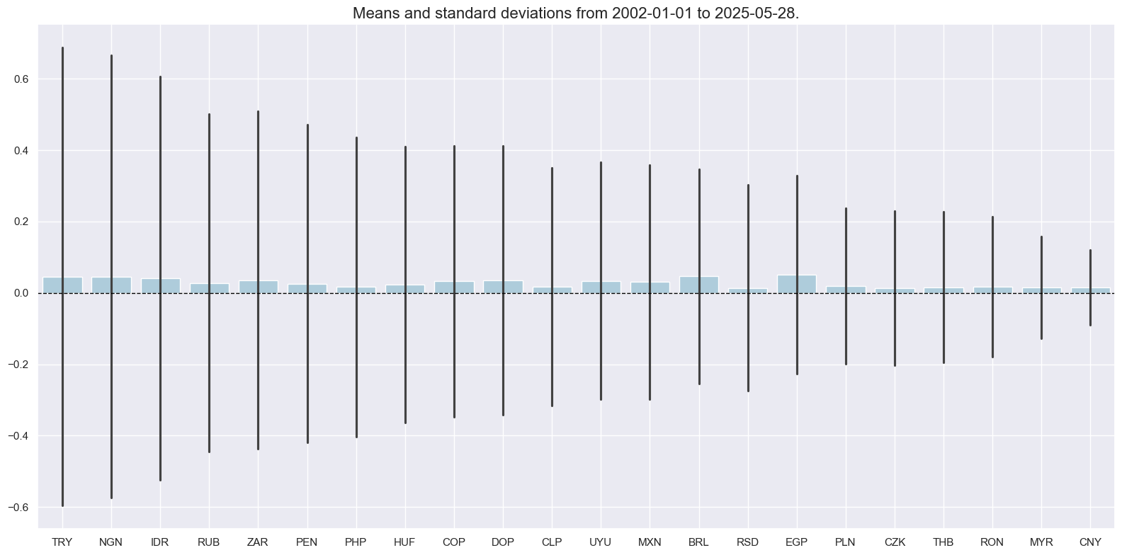
Daily local currency bond returns have displayed great differences in variance across countries. Standard deviations in Turkey, Indonesia, Nigeria, and Brail have been roughly 5 times as large as in China, for example.
xcatx = ["LCBIR_NSA"]
cidx = cids_lc
msp.view_ranges(
    dfd,
    xcats=xcatx,
    cids=cidx,
    sort_cids_by="std",
    start="2002-01-01",
    kind="bar",
    size=(16, 8),
)
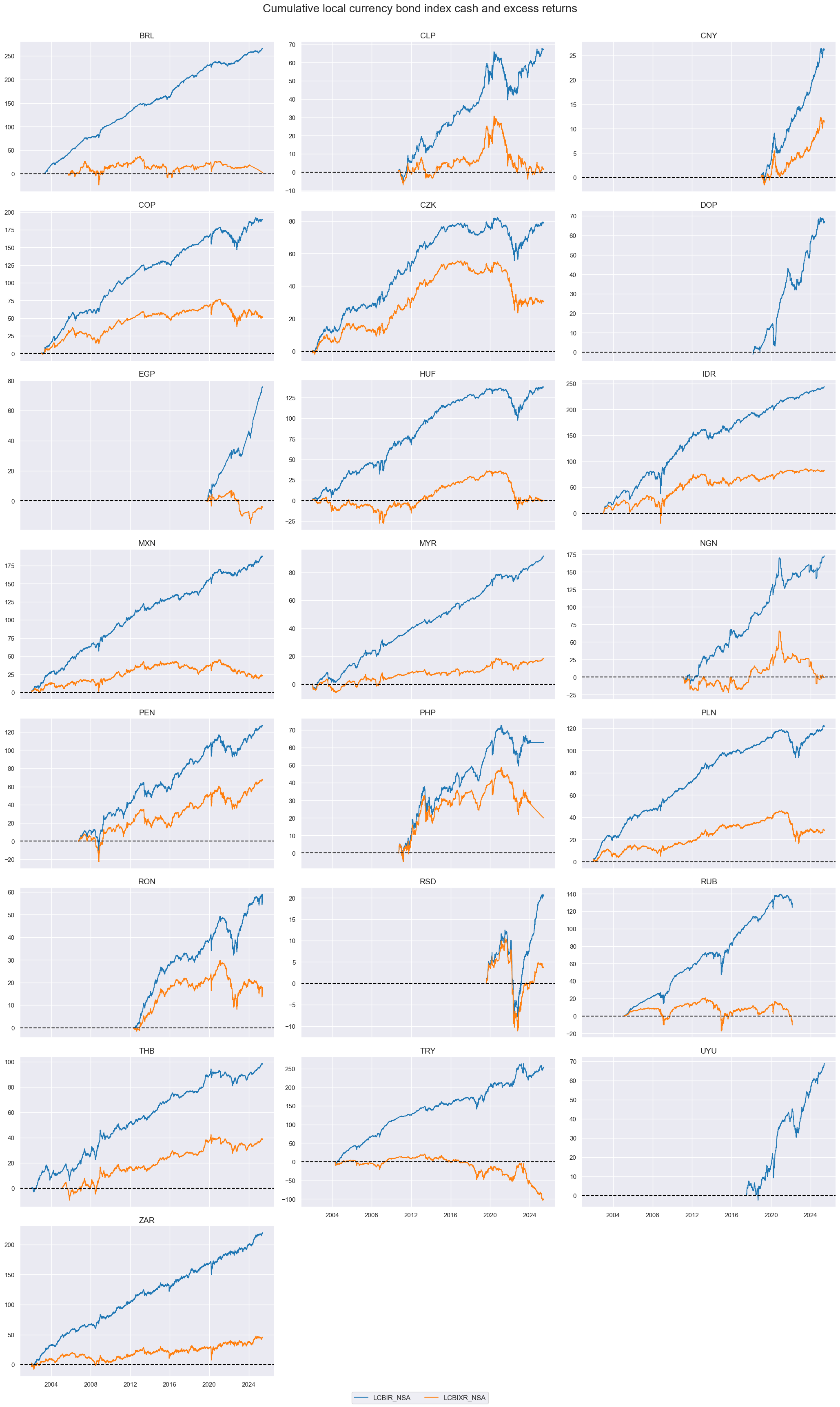
Long-term total returns in local currency have been positive for all countries. However, excess returns have been a lot more volatile and negative for a range of currency areas for the observed periods.
xcats_sel = ["LCBIR_NSA", "LCBIXR_NSA"]
cidx = cids_lc
msp.view_timelines(
    dfd,
    xcats=xcats_sel,
    cids=cidx,
    start="2000-01-01",
    title="Cumulative local currency bond index cash and excess returns",
    title_fontsize=20,
    cumsum=True,
    ncol=3,
    same_y=False,
)
plt.show()
xcats_sel = ["LCBIRUSD_NSA", "LCBIXRUSD_NSA"]
cidx = cids_lc
msp.view_timelines(
    dfd,
    xcats=xcats_sel,
    cids=cidx,
    start="2000-01-01",
    title="Cumulative local currency bond index cash and excess returns converted into USD",
    title_fontsize=20,
    cumsum=True,
    ncol=3,
    same_y=False,
)
plt.show()
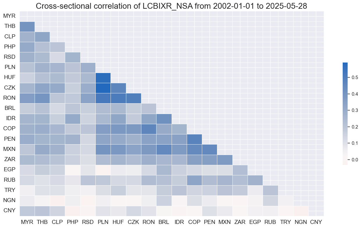
Cross-country correlation of weekly returns has been dominantly positive, but correlation coefficients have mostly been contained below 50%. Some countries posted more idiosyncratic returns dynamics.
cidx = cids_lc
msp.correl_matrix(
    dfd, xcats="LCBIXR_NSA", freq="W", cids=cids, cluster=True
)
Foreign currency bond cash returns #
Foreign-currency index returns have been more volatile than local currency returns. Differences in volatility across countries have large, but not quite as large as for local-currency bonds.
xcatx = ["FCBIR_NSA"]
cidx = cids_fc
msp.view_ranges(
    dfd,
    xcats=xcatx,
    cids=cidx,
    sort_cids_by="std",
    start="2002-01-01",
    kind="bar",
    size=(16, 8),
)
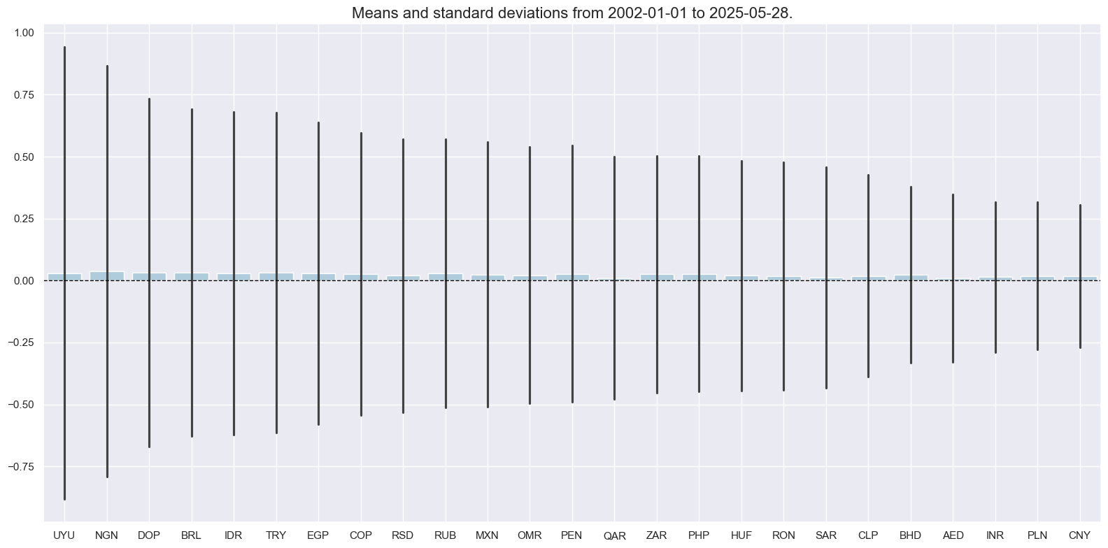
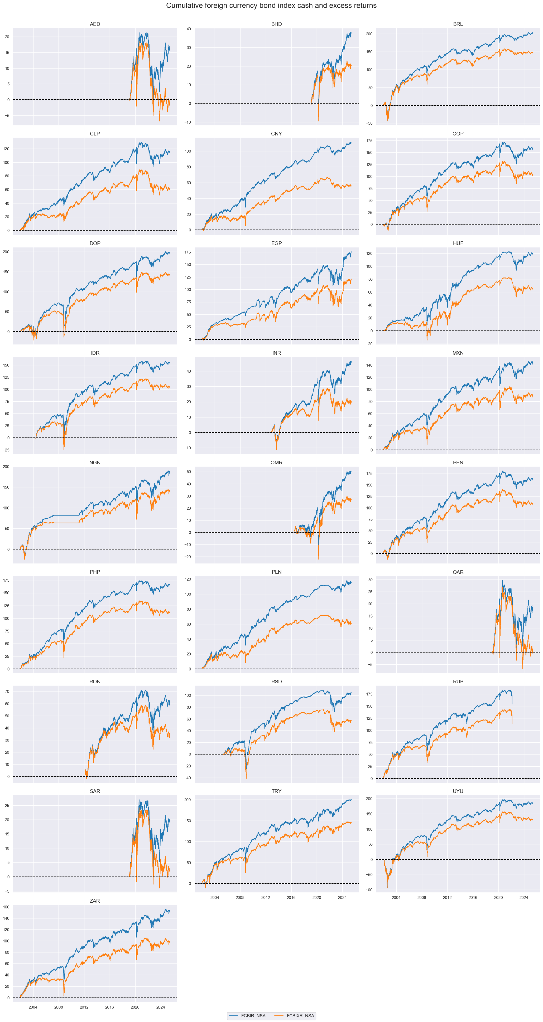
Most foreign currency bond indices have posted positive long-term returns, due partly to the decline in USD interest rates since 2000. However, return distribution has been heavily skewed to the downside.
xcats_sel = ["FCBIR_NSA", "FCBIXR_NSA"]
cidx = cids_fc
msp.view_timelines(
    dfd,
    xcats=xcats_sel,
    cids=cidx,
    start="2000-01-01",
    title="Cumulative foreign currency bond index cash and excess returns",
    title_fontsize=20,
    cumsum=True,
    ncol=3,
    same_y=False,
)
plt.show()
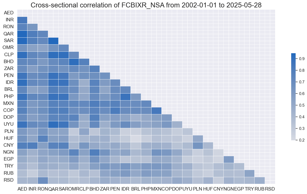
Cross-country correlation of weekly returns has been uniformly positive and much stronger than for local currency returns.
cidx = cids_fc
msp.correl_matrix(
    dfd, xcats="FCBIXR_NSA", freq="W", cids=cids, cluster=True
)
Importance #
Research Links #
“J.P. Morgan effective exchange rates are trade-weighted indices, focusing on the impact of currency fluctuations via international trade linkages.” Macrosynergy
“In emerging market economies, currency appreciation goes hand in hand with compressed sovereign bond spreads, even for local currency sovereign bonds. This yield compression comes from a reduction in the credit risk premium.” Bank of International Settlements
Empirical Clues #
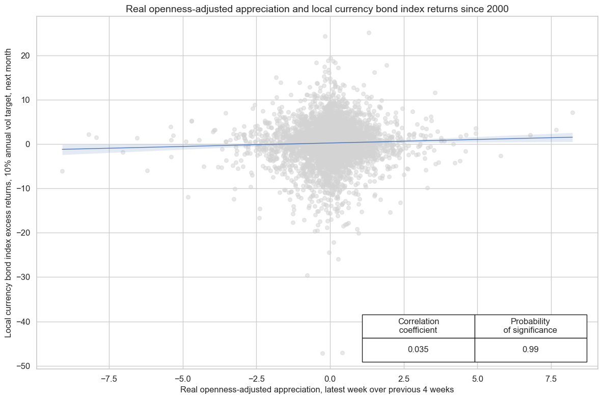
Openness-adjusted real real exchange rate dynamics help predict local inflation and policy rates. Also, there is a positive relation between improving investment conditions and capital inflows and real appreciation. Hence, it is not too surprising to find significant positive predictive power of openness-adjusted real appreciation for local currency bond returns.
cidx = cids_lc
xcatx = ["REEROADJ_NSA_P1W4WL1", "LCBIXR_VT10"]
cr = msp.CategoryRelations(
    dfd,
    xcats=xcatx,
    cids=cidx,
    freq="M",
    lag=1,
    slip=1,
    start="2000-01-01",
    years=None,
    xcat_aggs=["last", "sum"],
)
cr.reg_scatter(
    title="Real openness-adjusted appreciation and local currency bond index returns since 2000",
    labels=False,
    coef_box="lower right",
    ylab="Local currency bond index excess returns, 10% annual vol target, next month",
    xlab="Real openness-adjusted appreciation, latest week over previous 4 weeks",
    prob_est="map",
)
REEROADJ_NSA_P1W4WL1 misses: ['DOP', 'EGP', 'NGN', 'RSD', 'UYU'].
LCBIXR_VT10 misses: ['DOP', 'UYU'].
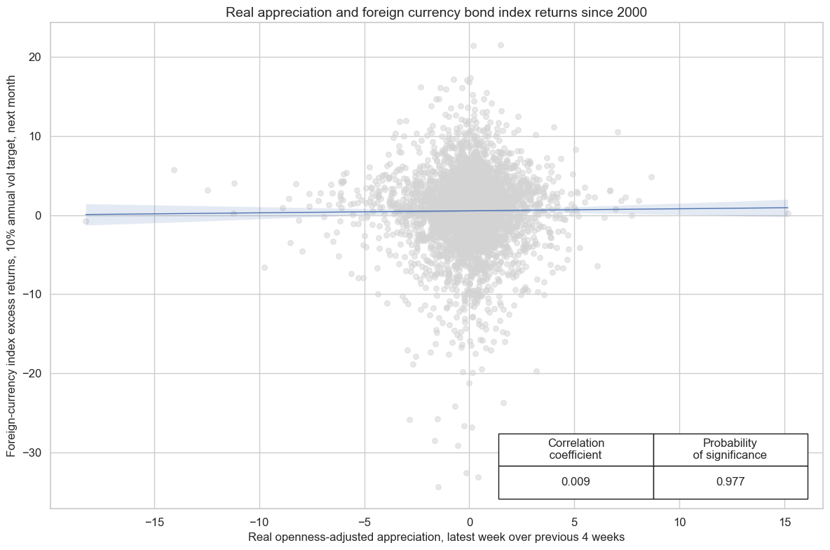
Interestingly, there has also been significant predictive power of the real effective exchange rate for foreign currency bond returns. Currency appreciation reduces the ratio of external debt service to GDP and is often a signal of improving investor sentiment.
cidx = cids_exp
xcatx = ["REER_NSA_P1W4WL1", "FCBIXR_VT10"]
cr = msp.CategoryRelations(
    dfd,
    xcats=xcatx,
    cids=cidx,
    freq="M",
    lag=1,
    slip=1,
    start="2000-01-01",
    years=None,
    xcat_aggs=["last", "sum"],
)
cr.reg_scatter(
    title="Real appreciation and foreign currency bond index returns since 2000",
    labels=False,
    coef_box="lower right",
    ylab="Foreign-currency index excess returns, 10% annual vol target, next month",
    xlab="Real openness-adjusted appreciation, latest week over previous 4 weeks",
    prob_est="map",
)
REER_NSA_P1W4WL1 misses: ['AED', 'BHD', 'DOP', 'EGP', 'NGN', 'OMR', 'QAR', 'RSD', 'SAR', 'UYU'].
FCBIXR_VT10 misses: ['CZK', 'MYR', 'THB'].
Appendices #
Appendix 1 #
Government Bond Index - Emerging Markets (GBI-EM) #
The J.P. Morgan Government Bond Index - Emerging Markets (GBI-EM) Indices provide investors with a benchmark that tracks local currency bonds issued by emerging market governments. The index was launched in June 2005 and is the first comprehensive global local Emerging Markets index.
As Emerging Market governments look increasingly toward their domestic market for sources of finance, investors continue to look more closely at local markets in search for higher yield and greater diversification. The GBI-EM Indices are comprised of only those countries from the GBI universe that meet the JP Morgan criteria for an Emerging Market, resulting in 22 countries from four regions.
For a country to be eligible for inclusion in the GBI-EM indices, GNI per capita must be below the Index Income Ceiling (IIC) for three consecutive years. J.P. Morgan defines the IIC as the GNI per capita level that is adjusted every year by the growth rate of the World GNI per capita, Atlas method (current US$), provided by the World Bank annually.
The GBI-EM consists of regularly traded, fixed-rate, domestic currency government bonds which international investors can readily access. JP Morgan determine eligibility for local currency issues using the following criteria: instrument type, current amount outstanding, liquidity, maturity. The GBI-EM indices only include fixed coupon instruments. Additionally, bonds with callable, puttable or convertible features are not part of the indices. Only instruments with a current face amount outstanding of US $1 billion equivalent for onshore local currency bonds and USD 500 million equivalent for global bonds (offshore currency linked bonds) or more will be considered for inclusion.
More information can be found in the documantation
EMBI Global (EMBIG) #
The J.P. Morgan Emerging Markets Bond Index Global (EMBIG) (and Emerging Markets Bond Index Global Diversified (EMBIGD) ) are J.P. Morgan’s most comprehensive US dollar emerging markets debt benchmarks. The EMBI suite of indices considers US dollar-denominated bonds issued by sovereign and quasi-sovereign EM entities eligible for inclusion.
The EMBI suite classifies countries as Emerging Markets or Developed Markets by applying a combination of income-based and purchasing power-based criteria. These multi-dimensional rules allow the EMBIG to include a number of higher-rated countries that international investors have nevertheless considered part of the emerging markets universe.
A country is eligible for inclusion to the EMBIG/EMBIGD if either the GNI per capita of the country’s economy is below the Index Income Ceiling (IIC) for three consecutive years or the nation’s cost of living (purchasing power) is below the Index PPP Ratio (IPR) for three consecutive years.
More information can be found in the documentation
Appendix 2 #
Return calculation #
The index calculation methodology is explained here.
Total return #
The total return calculation for a single instrument is a means of representing the economic benefit of holding the specific security. In its simplest form, it is based on the “cash in/cash out” notion-i.e., what is paid for the security at the initial purchase versus what is received at its sale. Of course, most fixed income securities pay some form of coupon along the way, and some pay amortizations. For the calculation of individual instrument total returns, this cash is reinvested in the instrument when received. However, when the instrument is part of a portfolio whose allocations are based on market capitalization (in the case of the EMBIG or the EMBIGD), the use of this market capitalization weighting scheme in effect causes this cash to be proportionately reinvested into the other instruments that make up the portfolio. Total return for an individual bond between days (t-1) and (t) is calculated as shown below, using daily local market clean prices and accrued interest:
Where: TR(t) = Bond total return from day (t-1) to day (t) including both principal and interest P(t) = Local market closing clean bid prices of a bond on day t AV(v(t)) = Accrued interest for a bond on day v(t), where the function v(t) are the value dates associated with trade date t and t-1 following market conventions.
When v(t) falls on a coupon date, the coupon will be added into the calculation of the total return, in effect reinvesting the coupon. As per market convention, on coupon date accrued interest is set to zero.
The total return index for individual bonds are calculated as shown below. At initiation, an index is given a base value of 100 and then daily returns are applied as shown below:
Where Index(t) is equal to the bond level total return index on day t and TR(t) is the total return on day t.
Bond specific information is aggregated to the portfolio level using weights. At the portfolio level, the total return of the index is the sum product of the individual bond returns and the individual bond weights of the previous day.
Where R(t) is equal to the index level return on day t and w(t-1) is the bond weight on day t-1.
This weighted return is then applied to the previous day’s index value as shown below:
Excess returns #
In order to calculate excess returns for the bond index, in a similar fashion to the methodology utilised for government bond excess returns, we take the daily return for the index and subtract from it the nominal interbank interest rate, de-annualised.
Where nir is the nominal interbank rate of that country.
Appendix 3: Currency symbols #
The word ‘cross-section’ refers to currencies, currency areas or economic areas. In alphabetical order, these are
-
AED (Emirates dirham)
-
AUD (Australian dollar)
-
BHD (Bahraini Dinar)
-
BRL (Brazilian real)
-
CAD (Canadian dollar)
-
CHF (Swiss franc)
-
CLP (Chilean peso)
-
CNY (Chinese yuan renminbi)
-
COP (Colombian peso)
-
CZK (Czech Republic koruna)
-
DEM (German mark)
-
DOP (Dominican Peso)
-
EGP (Egyptian Pound)
-
ESP (Spanish peseta)
-
EUR (Euro)
-
FRF (French franc)
-
GBP (British pound)
-
HKD (Hong Kong dollar)
-
HUF (Hungarian forint)
-
IDR (Indonesian rupiah)
-
ITL (Italian lira)
-
JPY (Japanese yen)
-
KRW (Korean won)
-
MXN (Mexican peso)
-
MYR (Malaysian ringgit)
-
NGN (Nigerian Naira)
-
NLG (Dutch guilder)
-
NOK (Norwegian krone)
-
NZD (New Zealand dollar)
-
OMR (Omani Rial)
-
QAR (Qatari Riyal)
-
PAB (Panamanian balboa)
-
PEN (Peruvian sol)
-
PHP (Phillipine peso)
-
PLN (Polish zloty)
-
RON (Romanian leu)
-
RSD (Serbian Dinar)
-
RUB (Russian ruble)
-
SEK (Swedish krona)
-
SAR (Saudi riyal)
-
SGD (Singaporean dollar)
-
THB (Thai baht)
-
TRY (Turkish lira)
-
TWD (Taiwanese dollar)
-
UYU (Peso Uruguayo)
-
USD (U.S. dollar)
-
VEF (Venezuelan bolívar)
-
ZAR (South African rand).