Economic openness ratios #
The category group contains semi-structural ratios of foreign trade as a ratio of the size of the economy. Effectively, they divide the sum of exports and imports (with and without services) by nominal GDP, based on concurrent data vintages.
The ratios are useful for the construction of trading factors that need to qualify the impact of external developments, such as foreign growth or effective exchange rate changes, on local economic and market developments.
Openness measured by merchandise external trade #
Ticker : EXMOPENNESS_NSA_1YMA
Label : External merchandise trade as ratio of GDP, 1-year moving average.
Definition : Sum of merchandise exports and imports, as ratio of concurrent estimated GDP, 1-year moving average.
Notes :
-
The merchandise trade data is taken from current account and customs trade reports.
-
The 1-year moving average of the nominal GDP is based on published quarterly national accounts with extrapolation up to the latest month for which the trade data has been released.
Openness measured by total external trade #
Ticker : EXALLOPENNESS_NSA_1YMA
Label : All external trade as ratio of GDP, 1-year moving average.
Definition : Sum of merchandise and services exports and imports, as ratio of GDP, 1-year moving average.
Notes :
-
The external merchandise and services trade data is taken from the national accounts.
-
The 1-year moving average of the nominal GDP is based on published quarterly national accounts.
Imports #
Only the standard Python data science packages and the specialized
macrosynergy
package are needed.
import os
import numpy as np
import pandas as pd
import matplotlib.pyplot as plt
import seaborn as sns
import math

import json
import yaml

import macrosynergy.management as msm
import macrosynergy.panel as msp
import macrosynergy.signal as mss
import macrosynergy.pnl as msn

from macrosynergy.download import JPMaQSDownload

from timeit import default_timer as timer
from datetime import timedelta, date, datetime

import warnings

warnings.simplefilter("ignore")
The
JPMaQS
indicators we consider are downloaded using the J.P. Morgan Dataquery API interface within the
macrosynergy
package. This is done by specifying
ticker strings
, formed by appending an indicator category code
<category>
to a currency area code
<cross_section>
. These constitute the main part of a full quantamental indicator ticker, taking the form
DB(JPMAQS,<cross_section>_<category>,<info>)
, where
<info>
denotes the time series of information for the given cross-section and category. The following types of information are available:
-
valuegiving the latest available values for the indicator -
eop_lagreferring to days elapsed since the end of the observation period -
mop_lagreferring to the number of days elapsed since the mean observation period -
gradedenoting a grade of the observation, giving a metric of real time information quality.
After instantiating the
JPMaQSDownload
class within the
macrosynergy.download
module, one can use the
download(tickers,start_date,metrics)
method to easily download the necessary data, where
tickers
is an array of ticker strings,
start_date
is the first collection date to be considered and
metrics
is an array comprising the times series information to be downloaded.
# Cross-sections of interest

cids_dmca = [
    "AUD",
    "CAD",
    "CHF",
    "EUR",
    "GBP",
    "JPY",
    "NOK",
    "NZD",
    "SEK",
    "USD",
]  # DM currency areas
cids_dmec = ["DEM", "ESP", "FRF", "ITL", "NLG"]  # DM euro area countries
cids_latm = ["BRL", "COP", "CLP", "MXN", "PEN"]  # Latam countries
cids_emea = ["CZK", "HUF", "ILS", "PLN", "RON", "RUB", "TRY", "ZAR"]  # EMEA countries
cids_emas = [
    "CNY",
    "IDR",
    "INR",
    "KRW",
    "MYR",
    "PHP",
    "SGD",
    "THB",
    "TWD",
]  # EM Asia countries

cids_dm = cids_dmca + cids_dmec
cids_em = cids_latm + cids_emea + cids_emas

cids = sorted(cids_dm + cids_em)
main = ["EXMOPENNESS_NSA_1YMA", "EXALLOPENNESS_NSA_1YMA"]

econ = [
    "FXXRxEASD_NSA",
    "EQXRxEASD_NSA",
]  # economic context

mark = [
    "FXXR_NSA",
    "FXXR_VT10",
    "FXXRHvGDRB_NSA",
    "EQXR_NSA",
    "EQXR_VT10",
    "FXTARGETED_NSA",
    "FXUNTRADABLE_NSA",
]  # market links

xcats = main + econ + mark
# Download series from J.P. Morgan DataQuery by tickers

start_date = "2000-01-01"
tickers = [cid + "_" + xcat for cid in cids for xcat in xcats]
print(f"Maximum number of tickers is {len(tickers)}")

# Retrieve credentials

client_id: str = os.getenv("DQ_CLIENT_ID")
client_secret: str = os.getenv("DQ_CLIENT_SECRET")

# Download from DataQuery

with JPMaQSDownload(client_id=client_id, client_secret=client_secret) as downloader:
    start = timer()
    df = downloader.download(
        tickers=tickers,
        start_date=start_date,
        metrics=["value", "eop_lag", "mop_lag", "grading"],
        suppress_warning=True,
        show_progress=True,
    )
    end = timer()

dfd = df

print("Download time from DQ: " + str(timedelta(seconds=end - start)))
Maximum number of tickers is 407
Downloading data from JPMaQS.
Timestamp UTC:  2025-04-02 11:27:22
Connection successful!
Requesting data: 100%|█████████████████████████████████████████████████████████████████| 82/82 [00:18<00:00,  4.47it/s]
Downloading data: 100%|████████████████████████████████████████████████████████████████| 82/82 [00:30<00:00,  2.72it/s]
Some expressions are missing from the downloaded data. Check logger output for complete list.
312 out of 1628 expressions are missing. To download the catalogue of all available expressions and filter the unavailable expressions, set `get_catalogue=True` in the call to `JPMaQSDownload.download()`.
Some dates are missing from the downloaded data.
3 out of 6590 dates are missing.
Download time from DQ: 0:00:54.206472
Availability #
cids_exp = sorted(cids)  # cids expected in category panels
msm.missing_in_df(dfd, xcats=main, cids=cids_exp)
No missing XCATs across DataFrame.
Missing cids for EXALLOPENNESS_NSA_1YMA:  ['CNY']
Missing cids for EXMOPENNESS_NSA_1YMA:    ['DEM', 'ESP', 'FRF', 'ITL', 'NLG']
Quantamental indicators of economic openness ratios are typically available by 2000. When both merchandise and services imports and exports are considered (
EXALLOPENNESS_NSA_1YMA
), Colombia, India and South Africa are notable late-starters.
For the explanation of currency symbols, which are related to currency areas or countries for which categories are available, please view Appendix 1 .
xcatx = main
cidx = cids_exp

dfx = msm.reduce_df(dfd, xcats=xcatx, cids=cidx)
dfs = msm.check_startyears(
    dfx,
)
msm.visual_paneldates(dfs, size=(18, 2))

print("Last updated:", date.today())

Last updated: 2025-04-02
xcatx = main
cidx = cids_exp

plot = msm.check_availability(
    dfd, xcats=xcatx, cids=cidx, start_size=(18, 4), start_years=False
)

Average vintage grading is more varied for openness measured by total external trade than openness measured by merchandise external trade, for which perfect grades are attained in almost all developed markets.
xcatx = main
cidx = cids_exp

plot = msp.heatmap_grades(
    dfd,
    xcats=xcatx,
    cids=cidx,
    size=(18, 2),
    title=f"Average vintage grades from {start_date} onwards",
)

xcatx = main
cidx = cids_exp

msp.view_ranges(
    dfd,
    xcats=xcatx,
    cids=cidx,
    val="eop_lag",
    title="End of observation period lags (ranges of time elapsed since end of observation period in days)",
    start="2002-01-01",
    kind="box",
    size=(16, 4),
)
msp.view_ranges(
    dfd,
    xcats=xcatx,
    cids=cidx,
    val="mop_lag",
    title="Median of observation period lags (ranges of time elapsed since middle of observation period in days)",
    start="2002-01-01",
    kind="box",
    size=(16, 4),
)


History #
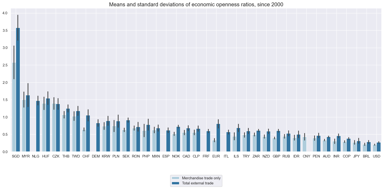
Merchandise trade-to-GDP ratios have averaged between 10% and 260% of GDP across currency areas since 2000, underscoring the vast differences of the effects of exchange rate movements on financial conditions. In comparison, total goods and services external trade ratios have averaged between 25% and 360% of GDP. Notably, the Euro area exhibits far greater openness when including services trade data.
xcatx = ["EXMOPENNESS_NSA_1YMA", "EXALLOPENNESS_NSA_1YMA"]
cidx = cids_exp

msp.view_ranges(
    dfd,
    xcats=xcatx,
    cids=cidx,
    sort_cids_by="mean",
    start="2000-01-01",
    kind="bar",
    title="Means and standard deviations of economic openness ratios, since 2000",
    xcat_labels=["Merchandise trade only", "Total external trade"],
    size=(16, 8),
)

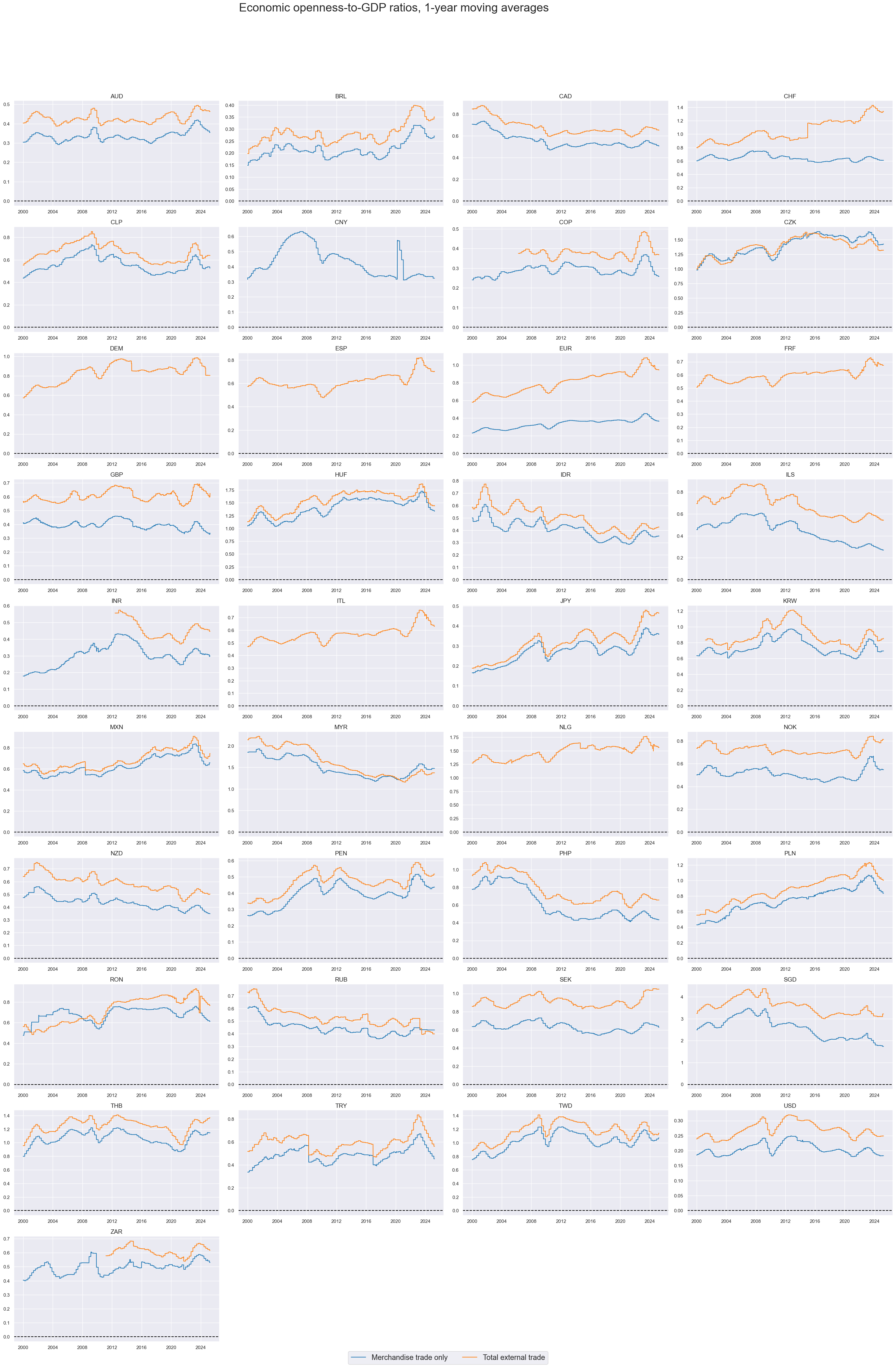
The vast majority of economic openness ratio indicators are slow-moving and some countries posted pronounced secular trends. Indeed, fluctuations have been modest compared to their absolute sizes and differences.
xcatx = ["EXMOPENNESS_NSA_1YMA", "EXALLOPENNESS_NSA_1YMA"]
cidx = cids_exp

msp.view_timelines(
    dfd,
    xcats=xcatx,
    cids=cidx,
    start="2000-01-01",
    title="Economic openness-to-GDP ratios, 1-year moving averages",
    title_adj=1.03,
    title_fontsize=27,
    legend_fontsize=17,
    label_adj=0.075,
    title_xadj=0.44,
    xcat_labels=["Merchandise trade only", "Total external trade"],
    ncol=4,
    same_y=False,
    size=(12, 7),
    aspect=1.7,
    all_xticks=True,
)

Importance #
Research links #
“Differences in the trade openness explain a large part of the cross-country variation in the volatility of the real exchange rate…Economic openness and exchange rate volatility are inversely related.” Hau
“Using a dataset of 101 countries over the 1960–2011 period, we examine the relationship between the real effective exchange rate (REER), on the one hand, and trade openness…on the other…The findings of the study strongly support the hypothesis that an increase in trade openness produces a depreciation of the REER.” Hau
“Our findings support existing theoretical models…(and) confirm empirically that the composition of trade and financial openness matters for real exchange rate stabilization. We show that trade in manufacturing helps reduce real exchange rate volatility while non-manufacturing trade may contribute to higher real exchange rate volatility.” Calderón and Kubota
Empirical clues #
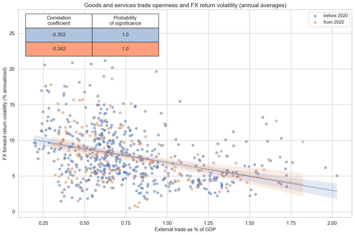
As predicted by theory, economic openness has been negatively related to FX return volatility. This relation prevailed both before and after the COVID-19 pandemic.
dfb = dfd[dfd["xcat"].isin(["FXTARGETED_NSA", "FXUNTRADABLE_NSA"])].loc[
    :, ["cid", "xcat", "real_date", "value"]
]
dfba = (
    dfb.groupby(["cid", "real_date"])
    .aggregate(value=pd.NamedAgg(column="value", aggfunc="max"))
    .reset_index()
)
dfba["xcat"] = "FXBLACK"
fxblack = msp.make_blacklist(dfba, "FXBLACK")
fxblack
{'BRL': (Timestamp('2012-12-03 00:00:00'), Timestamp('2013-09-30 00:00:00')),
 'CHF': (Timestamp('2011-10-03 00:00:00'), Timestamp('2015-01-30 00:00:00')),
 'CNY': (Timestamp('2000-01-03 00:00:00'), Timestamp('2025-04-01 00:00:00')),
 'CZK': (Timestamp('2014-01-01 00:00:00'), Timestamp('2017-07-31 00:00:00')),
 'ILS': (Timestamp('2000-01-03 00:00:00'), Timestamp('2005-12-30 00:00:00')),
 'INR': (Timestamp('2000-01-03 00:00:00'), Timestamp('2004-12-31 00:00:00')),
 'MYR_1': (Timestamp('2000-01-03 00:00:00'), Timestamp('2007-11-30 00:00:00')),
 'MYR_2': (Timestamp('2018-07-02 00:00:00'), Timestamp('2025-04-01 00:00:00')),
 'PEN': (Timestamp('2021-07-01 00:00:00'), Timestamp('2021-07-30 00:00:00')),
 'RON': (Timestamp('2000-01-03 00:00:00'), Timestamp('2005-11-30 00:00:00')),
 'RUB_1': (Timestamp('2000-01-03 00:00:00'), Timestamp('2005-11-30 00:00:00')),
 'RUB_2': (Timestamp('2022-02-01 00:00:00'), Timestamp('2025-04-01 00:00:00')),
 'SGD': (Timestamp('2000-01-03 00:00:00'), Timestamp('2025-04-01 00:00:00')),
 'THB': (Timestamp('2007-01-01 00:00:00'), Timestamp('2008-11-28 00:00:00')),
 'TRY_1': (Timestamp('2000-01-03 00:00:00'), Timestamp('2003-09-30 00:00:00')),
 'TRY_2': (Timestamp('2020-01-01 00:00:00'), Timestamp('2024-07-31 00:00:00'))}
xcatx = ["EXALLOPENNESS_NSA_1YMA", "FXXRxEASD_NSA"]
cidx = list(set(cids_exp) - set(["CNY", "USD"]))

cr_crr = msp.CategoryRelations(
    dfd,
    xcats=xcatx,
    cids=cidx,
    freq="A",
    lag=0,
    xcat_aggs=["mean", "mean"],
    start="2000-01-01",
    # years=10,
    blacklist=fxblack,
)
cr_crr.reg_scatter(
    title="Goods and services trade openness and FX return volatility (annual averages)",
    # labels=True,
    coef_box="upper left",
    xlab="External trade as % of GDP",
    ylab="FX forward return volatility (% annualized)",
    separator=2020,
)
FXXRxEASD_NSA misses: ['DEM', 'ESP', 'FRF', 'ITL', 'NLG'].

Appendices #
Appendix 1: Currency symbols #
The word ‘cross-section’ refers to currencies, currency areas or economic areas. In alphabetical order, these are AUD (Australian dollar), BRL (Brazilian real), CAD (Canadian dollar), CHF (Swiss franc), CLP (Chilean peso), CNY (Chinese yuan renminbi), COP (Colombian peso), CZK (Czech Republic koruna), DEM (German mark), ESP (Spanish peseta), EUR (Euro), FRF (French franc), GBP (British pound), HKD (Hong Kong dollar), HUF (Hungarian forint), IDR (Indonesian rupiah), ITL (Italian lira), JPY (Japanese yen), KRW (Korean won), MXN (Mexican peso), MYR (Malaysian ringgit), NLG (Dutch guilder), NOK (Norwegian krone), NZD (New Zealand dollar), PEN (Peruvian sol), PHP (Phillipine peso), PLN (Polish zloty), RON (Romanian leu), RUB (Russian ruble), SEK (Swedish krona), SGD (Singaporean dollar), THB (Thai baht), TRY (Turkish lira), TWD (Taiwanese dollar), USD (U.S. dollar), ZAR (South African rand).