Domestic credit ratios

This category group focuses on a variety of credit metrics in the local economy, as a ratio to GDP. Credit ratios are highly autocorrelated semi-structural indicators, often indicative of system vulnerability to increases in financial conditions.

Private credit-to-GDP ratios (local convention)

Ticker : PCREDITGDP_SA

Label : Private credit as % of GDP

Definition : Stock of private bank credit at the end of the latest reported month as % of 1-year moving average of nominal GDP.

Notes :

• This indicator is based on the most prominent private credit indicator by local convention. Unlike the other credit ratios of this category group, its definition is not exactly the same across all currency areas. For most countries, the numerator of the ratio refers to both bank loans to private households, and companies. Exceptions are AUD/Australia (narrow credit aggregate excluding securitization), BRL/Brazil (total bank credit), CHF/Switzerland (total bank loans), CNY/China (total domestic credit to non-financial sector), INR/India (domestic credit to commercial sector), JPY/Japan (loans and discounts outstanding, excluding Shinkin banks), THB/Thailand (all domestic claims), TWD/Taiwan (all loans and discounts), USD/ U.S. (all bank loans and leases).

• For Singapore, changes in reporting standards led to a series break between June and July 2021. Singapore’s monetary authority did not provide data for the new standard, but they reported that the underlying trends of new and old standards would be broadly similar. In light of this, JPMaQS revised the data history on the first reporting day of the new standard by setting the final value of the old series equal to the first value of the new series.

• The 1-year moving average of the nominal GDP is based on published quarterly national accounts with trend extrapolation up to the latest month for which private credit has been released.

Domestic credit-to-GDP ratios

Ticker : DCREDITGDP_NSA

Label : Total domestic credit as % of GDP.

Definition : Stock of total domestic credit, latest reported level, as % of 1-year moving average of nominal GDP

Notes :

• The numerator (credit aggregate) is the total amount of credit supplied by all banks (including the central bank) and non-banks to the domestic private non-financial sector and the government. Credit can be granted in form of loans, debt securities or deposits. Hence, this is a very broad concept. For most countries, the number is based on quarterly BIS statistics and defined as the stock at the end of the quarter. The BIS series are released with a 6-9 months lag to the end of the observation period but conveniently adjusted for breaks. For some countries, only net credit from monetary-financial institutions is available.

• The 1-year moving average of the nominal GDP is based on published quarterly national accounts with trend extrapolation up to the latest month for which the credit aggregate has been released.

Domestic private credit-to-GDP ratios

Ticker : DPCREDITGDP_NSA

Label : Domestic private credit as % of GDP

Definition : Stock of domestic credit to households and companies, latest reported level, as % of 1-year moving average of nominal GDP.

Notes :

• The numerator is the total amount of credit supplied by all banks and non-banks to the domestic private non-financial sector. Credit can be granted in the form of loans, debt securities or deposits. Hence, this is a very broad concept for private credit. For most countries, the number is based on quarterly BIS statistics and defined as the stock at the end of the quarter. The BIS series are released with a 6-9 month lag to the end of the observation period but are conveniently adjusted for breaks. For some countries, only net credit from monetary-financial institutions is available.

Domestic private bank credit-to-GDP ratios

Ticker : DPBCREDITGDP_NSA

Label : Domestic private bank credit-to-GDP ratio in %.

Definition : Stock of bank loans to households and companies at the end of the latest reported month as % of 1-year moving average of nominal GDP.

Notes :

• The numerator is the total amount of credit supplied by banks to the domestic private non-financial sector. Credit can be granted in the form of loans, debt securities or deposits. For most countries, the number is based on quarterly BIS statistics and defined as the stock at the end of the quarter. The BIS series are released with a 6-9 month lag to the end of the observation period, but are conveniently adjusted for breaks.

• The indicator is often similar to the main private credit-to-GDP ratio but is defined consistently across countries or currency areas. It thereby trades timeliness and conventional focus for consistency.

• The 1-year moving average of the nominal GDP is based on published quarterly national accounts with trend extrapolation up to the latest month for which private credit has been released.

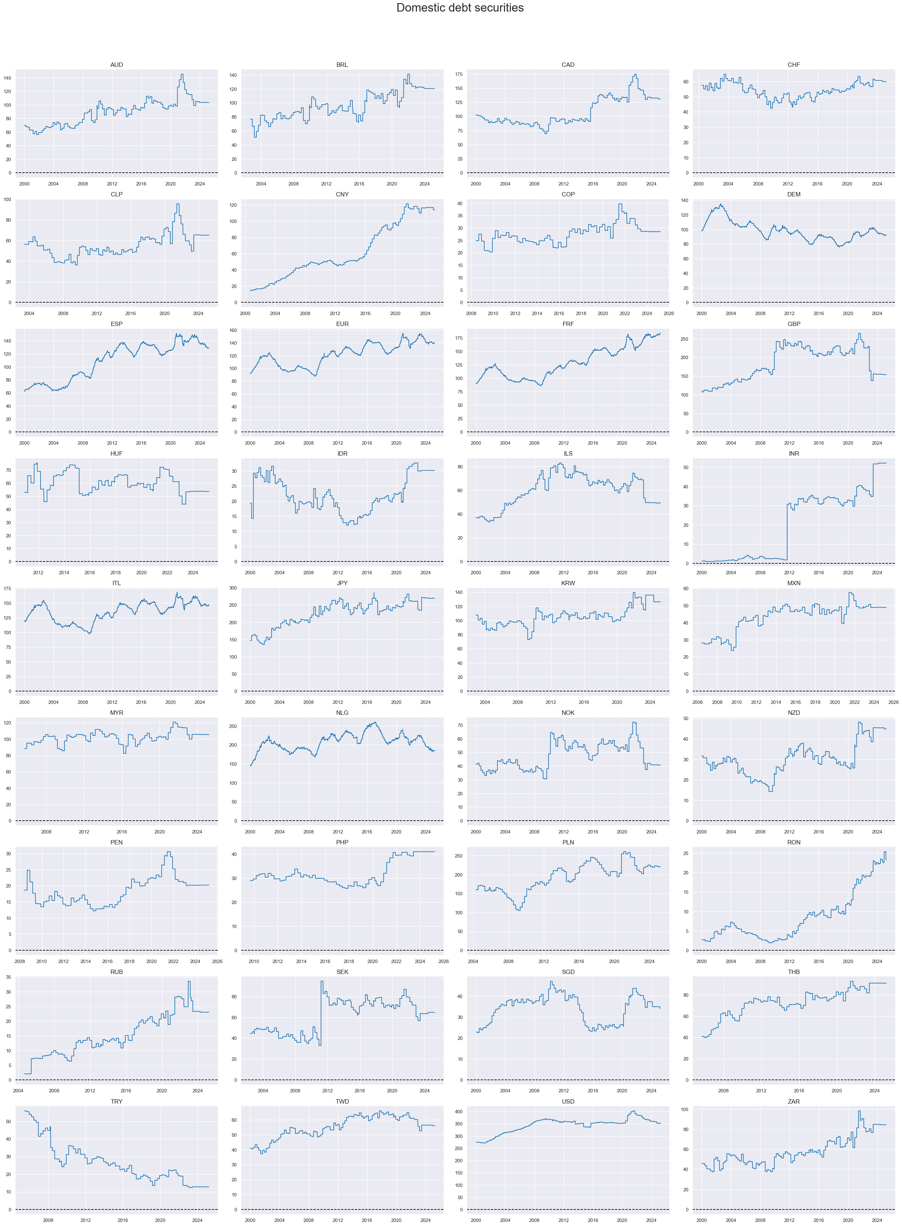
Domestic debt securities-to-GDP ratios

Ticker : DDEBTSECSGDP_NSA

Label : Ratio of all domestic debt securities to GDP in %.

Definition : Stock of all domestic debt securities at the end of the latest reported month as % of 1-year moving average of nominal GDP

Notes :

• The numerator is the total value of all domestic debt scurities, across all currencies, maturities and obligors.

• The 1-year moving average of the nominal GDP is based on published quarterly national accounts with trend extrapolation up to the latest month for which private credit has been released.

Imports

Only the standard Python data science packages and the specialized macrosynergy package are needed.

import os
import numpy as np
import pandas as pd
import matplotlib.pyplot as plt
import seaborn as sns
import math

import json

import macrosynergy.management as msm
import macrosynergy.panel as msp
import macrosynergy.signal as mss
import macrosynergy.pnl as msn


from macrosynergy.download import JPMaQSDownload

from timeit import default_timer as timer
from datetime import timedelta, date, datetime

import warnings

warnings.simplefilter("ignore")

The JPMaQS indicators we consider are downloaded using the J.P. Morgan Dataquery API interface within the macrosynergy package. This is done by specifying ticker strings , formed by appending an indicator category code <category> to a currency area code <cross_section> . These constitute the main part of a full quantamental indicator ticker, taking the form DB(JPMAQS,<cross_section>_<category>,<info>) , where <info> denotes the time series of information for the given cross-section and category. The following types of information are available:

• value giving the latest available values for the indicator

• eop_lag referring to days elapsed since the end of the observation period

• mop_lag referring to the number of days elapsed since the mean observation period

• grade denoting a grade of the observation, giving a metric of real time information quality.

After instantiating the JPMaQSDownload class within the macrosynergy.download module, one can use the download(tickers,start_date,metrics) method to easily download the necessary data, where tickers is an array of ticker strings, start_date is the first collection date to be considered and metrics is an array comprising the times series information to be downloaded.

# Define cross sections (currency tickers)

cids_dm = ["AUD", "CAD", "CHF", "EUR", "GBP", "JPY", "NOK", "NZD", "SEK", "USD"]
cids_dmec = ["DEM", "ESP", "FRF", "ITL", "NLG"]
cids_latm = ["BRL", "COP", "CLP", "MXN", "PEN"]
cids_emea = ["CZK", "HUF", "ILS", "PLN", "RON", "RUB", "TRY", "ZAR"]
cids_emas = ["CNY", "HKD", "IDR", "INR", "KRW", "MYR", "PHP", "SGD", "THB", "TWD"]
cids_em = cids_latm + cids_emea + cids_emas

cids = sorted(cids_dm + cids_em)

# Define quantamental indicators (category tickers)

main = [
    "PCREDITGDP_SA",
    "DCREDITGDP_NSA",
    "DPCREDITGDP_NSA",
    "DPBCREDITGDP_NSA",
    "DDEBTSECSGDP_NSA",
]
econ = [
    "RIR_NSA",
    "EQCRY_NSA",
    "FXUNTRADABLE_NSA",
    "FXTARGETED_NSA",
]  # economic context
mark = [
    "EQXR_NSA",
    "EQXR_VT10",
    "DU05YXR_NSA",
    "DU05YXR_VT10",
    "FXXR_NSA",
    "FXXR_VT10",
    "FXXRHvGDRB_NSA",
]  # market links

xcats = main + econ + mark

# Download series from J.P. Morgan DataQuery by tickers

start_date = "1990-01-01"
tickers = [cid + "_" + xcat for cid in cids for xcat in xcats]
print(f"Maximum number of tickers is {len(tickers)}")

# Retrieve credentials

client_id: str = os.getenv("DQ_CLIENT_ID")
client_secret: str = os.getenv("DQ_CLIENT_SECRET")

# Download from DataQuery

with JPMaQSDownload(client_id=client_id, client_secret=client_secret) as downloader:
    start = timer()
    df = downloader.download(
        tickers=tickers,
        start_date=start_date,
        show_progress=True,
        report_time_taken=True,
        metrics=["value", "eop_lag", "mop_lag", "grading"],
        suppress_warning=True,
    )
    end = timer()

dfd = df

print("Download time from DQ: " + str(timedelta(seconds=end - start)))

Maximum number of tickers is 528
Downloading data from JPMaQS.
Timestamp UTC:  2023-09-07 11:53:33
Connection successful!
Number of expressions requested: 2112

Requesting data: 100%|███████████████████████████████████████████████████████████████| 106/106 [00:34<00:00,  3.11it/s]
Downloading data: 100%|██████████████████████████████████████████████████████████████| 106/106 [01:05<00:00,  1.62it/s]

Time taken to download data: 	100.53 seconds.
Time taken to convert to dataframe: 	50.39 seconds.
Download time from DQ: 0:02:30.927467

Availability

cids_exp = sorted(
    list(set(cids) - set(cids_dmec + ["ARS", "HKD", "CZK"]))
)  # cids expected in category panels
msm.missing_in_df(dfd, xcats=main, cids=cids_exp)

Missing xcats across df:  []
Missing cids for DCREDITGDP_NSA:  []
Missing cids for DDEBTSECSGDP_NSA:  []
Missing cids for DPBCREDITGDP_NSA:  []
Missing cids for DPCREDITGDP_NSA:  []
Missing cids for PCREDITGDP_SA:  []

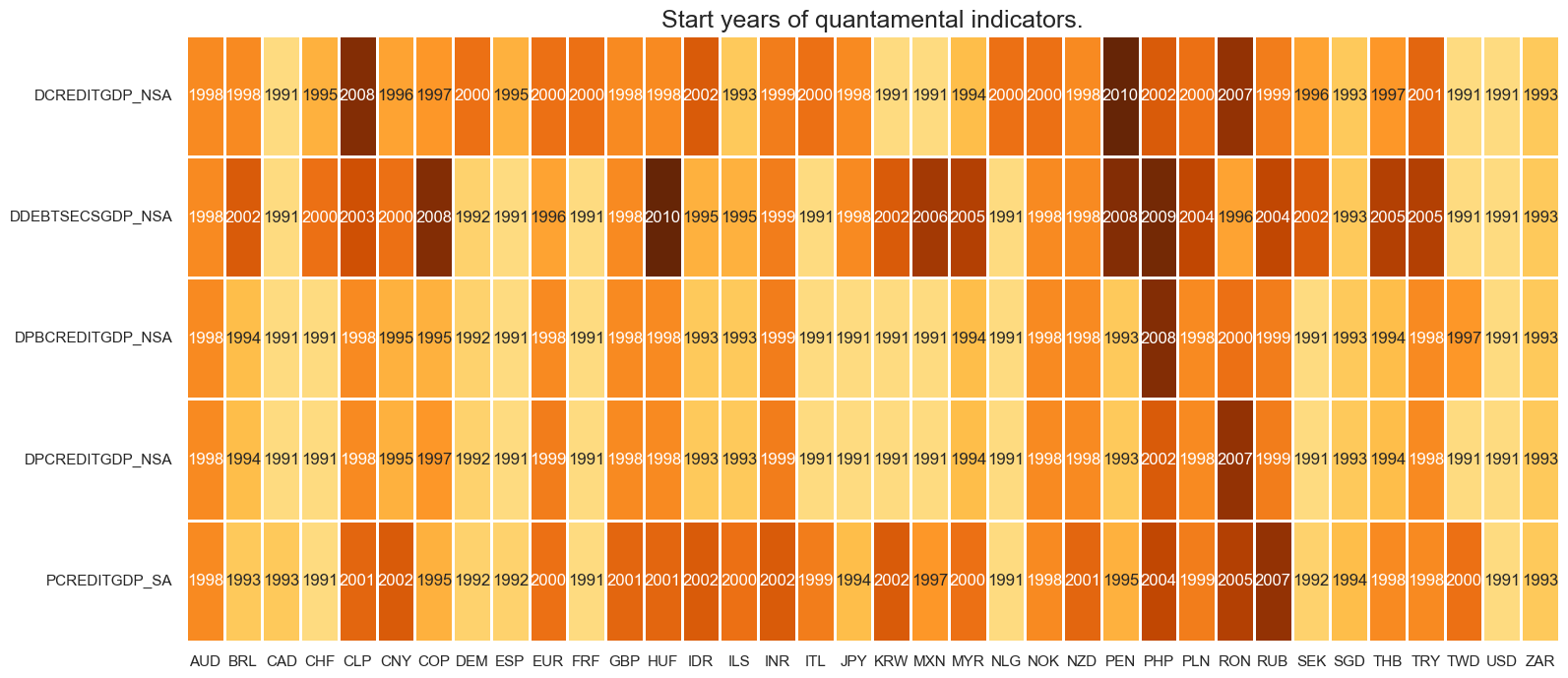
Most real-time quantamental indicators of domestic credit ratios are available from the 1990s. In general, the domestic debt security indicators are available later, from 2000 onwards.

For the explanation of currency symbols, which are related to currency areas or countries for which categories are available, please view Appendix 1 .

xcatx = main
cidx = cids_exp

dfx = msm.reduce_df(dfd, xcats=xcatx, cids=cidx)
dfs = msm.check_startyears(
    dfx,
)
msm.visual_paneldates(dfs, size=(18, 8))

print("Last updated:", date.today())

Last updated: 2023-09-07

xcatx = main
cidx = cids_exp

plot = msm.check_availability(
    dfd, xcats=xcatx, cids=cidx, start_size=(18, 8), start_years=False
)

Average vintage grading is low across most indicator categories and cross-sections. The private credit indicator category is consistently higher graded than the others, across all currency areas.

plot = msp.heatmap_grades(
    dfd,
    xcats=main,
    cids=cids_exp,
    size=(19, 2),
    title=f"Average vintage grades for each consistent core CPI category and each currency area, from {start_date} onwards",
)

msp.view_ranges(
    dfd,
    xcats=main,
    cids=cids_exp,
    val="eop_lag",
    title="End of observation period lags (ranges of time elapsed since end of observation period in days)",
    start=start_date,
    kind="box",
    size=(16, 4),
)
msp.view_ranges(
    dfd,
    xcats=main,
    cids=cids_exp,
    val="mop_lag",
    title="Median of observation period lags (ranges of time elapsed since end of observation period in days)",
    start=start_date,
    kind="box",
    size=(16, 4),
)

History

Private credit-to-GDP ratio (local convention)

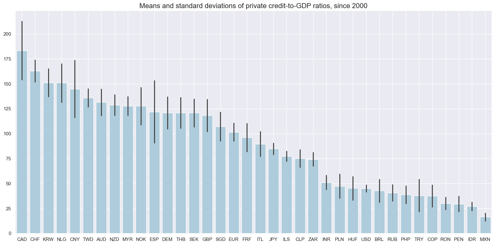
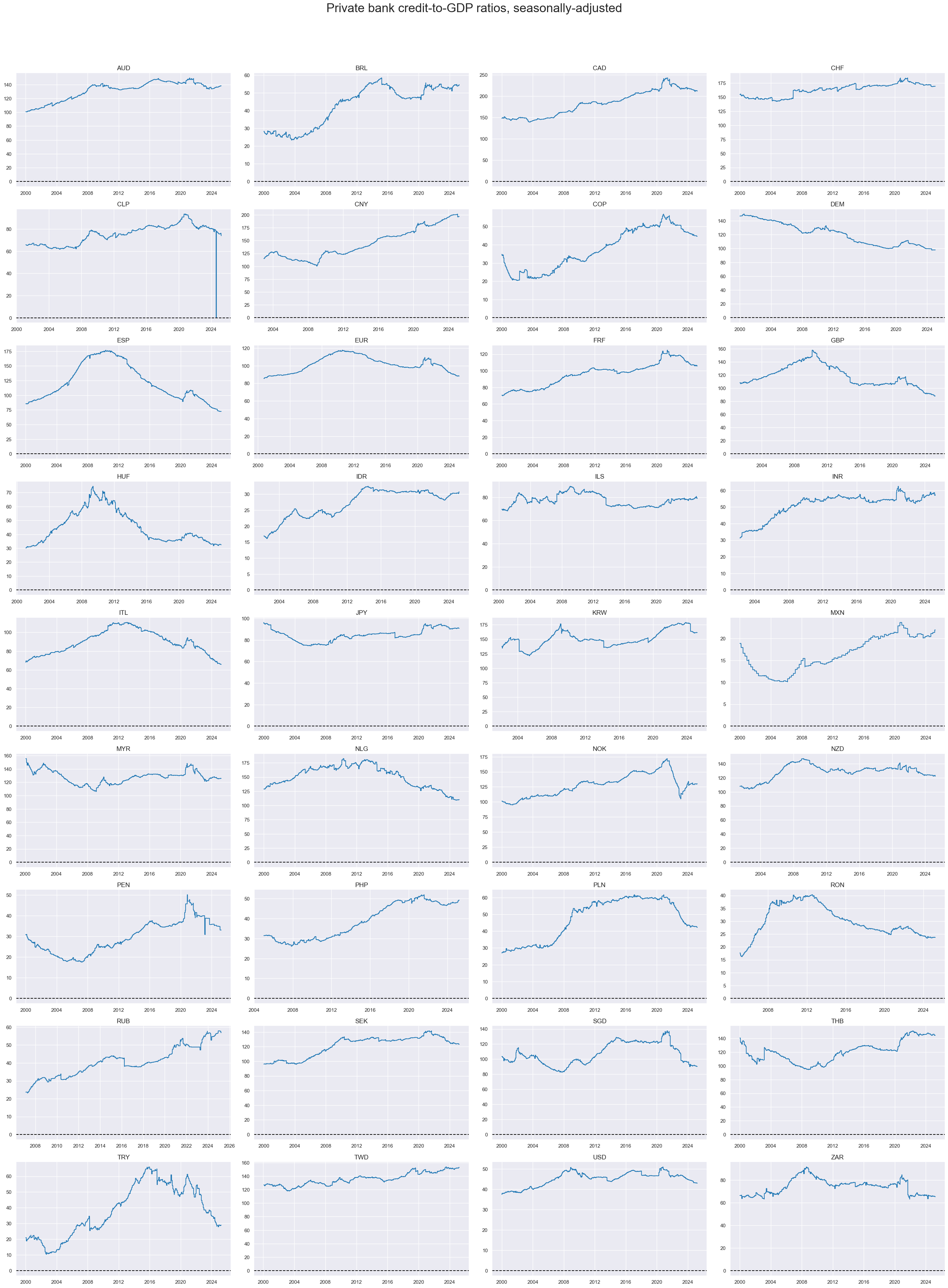
Over the last 20 years, the mean conventional ratios have varied substantially over cross-sections, from 15% to over 175% of their respective nominal GDPs. Differences in these indicators across cross-sections are not only due to changes in leverage provided by banks, but also due to local conventions and accounting rules. Hence, this indicator category is more suited as a basis to compare changes in the ratio (due to its timely release) than a basis to compare structural ratios.

xcatx = ["PCREDITGDP_SA"]
cidx = cids_exp

msp.view_ranges(
    dfd,
    xcats=xcatx,
    cids=cidx,
    sort_cids_by="mean",
    kind="bar",
    size=(16, 8),
    title="""Means and standard deviations of private credit-to-GDP ratios, since 2000""",
    start="2000-01-01",
)

xcatx = ["PCREDITGDP_SA"]
cidx = cids_exp

msp.view_timelines(
    dfd,
    xcats=xcatx,
    cids=cidx,
    start="2000-01-01",
    title="Private bank credit-to-GDP ratios, seasonally-adjusted",
    title_adj=1.02,
    title_xadj=0.5,
    title_fontsize=27,
    ncol=4,
    same_y=False,
    aspect=1.7,
    all_xticks=True,
    size=(16, 8),
)

Domestic total and private credit ratios

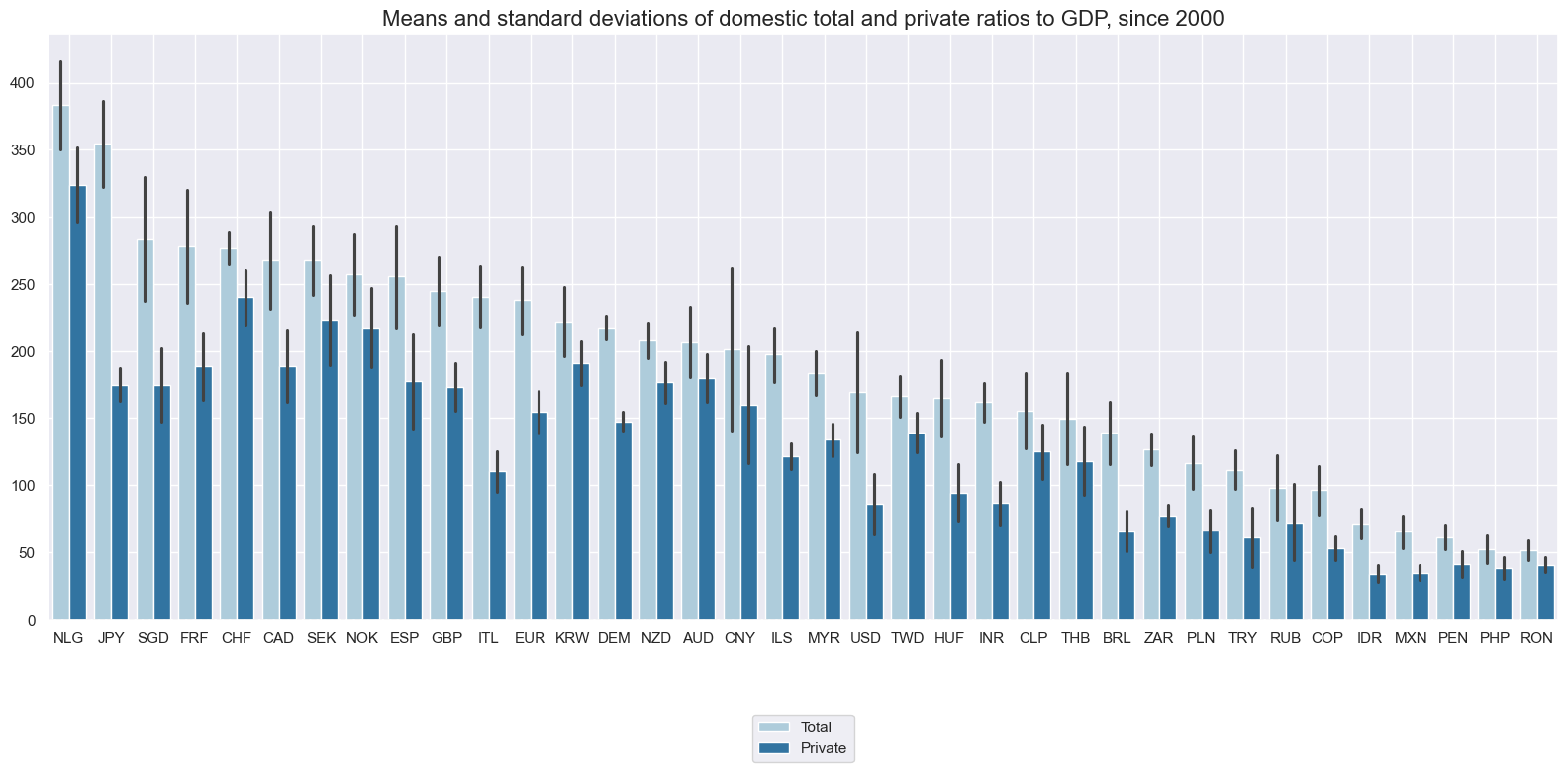
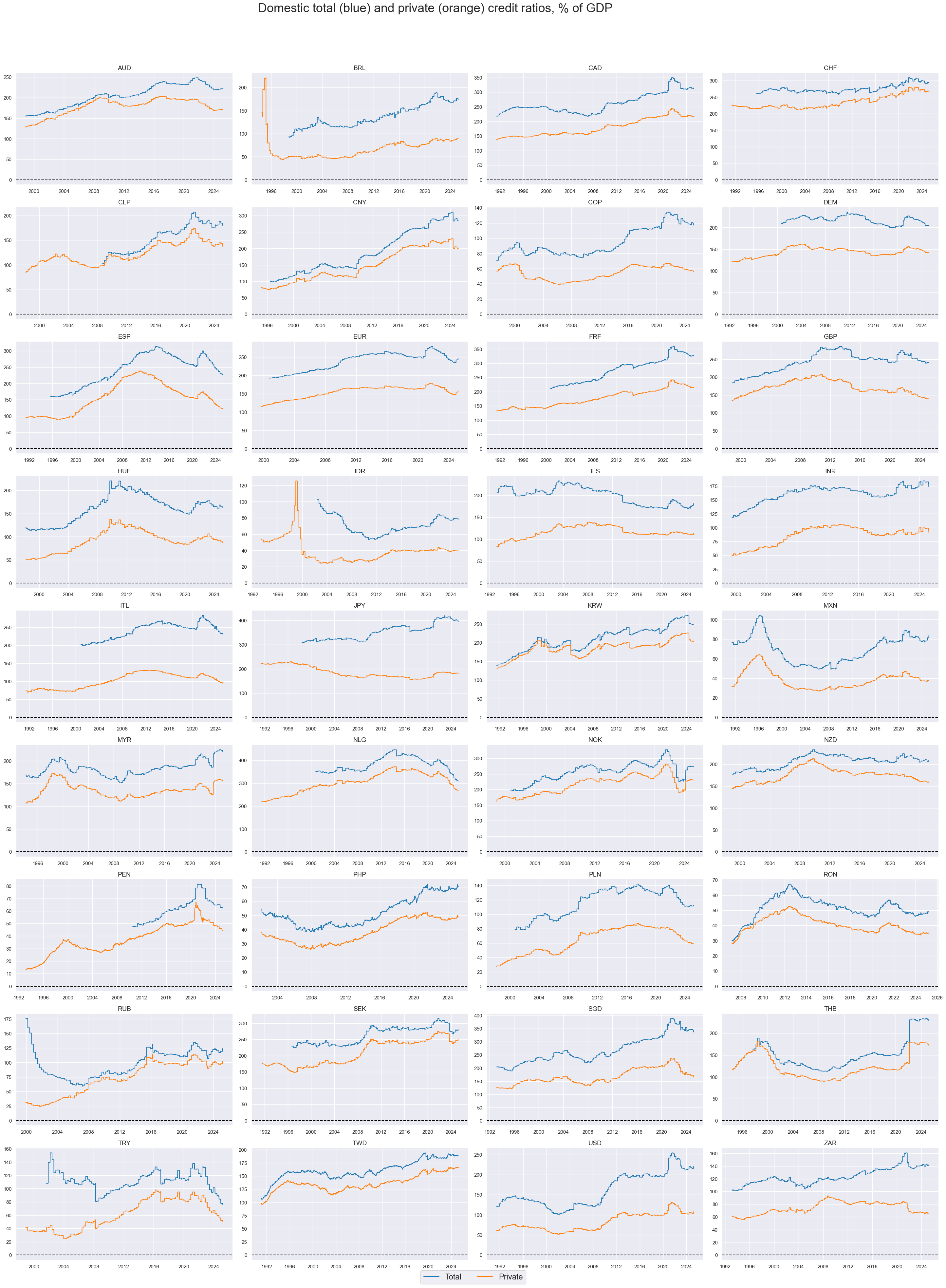
Average total credit ratios since 2000 have also been quite diverse, ranging from 30% to 350% of the nominal GDP. The relative importance of credit to the public and private sectors has been similarly diverse. Whilst the broad developments of total and private credit have been similar across time, they have displayed very different dynamics in some countries and episodes.

xcatx = ["DCREDITGDP_NSA", "DPCREDITGDP_NSA"]
cidx = cids_exp

msp.view_ranges(
    dfd,
    xcats=xcatx,
    cids=cidx,
    sort_cids_by="mean",
    kind="bar",
    title="Means and standard deviations of domestic total and private ratios to GDP, since 2000",
    xcat_labels=["Total", "Private"],
    start="2000-01-01",
    size=(16, 8),
)

xcatx = ["DCREDITGDP_NSA", "DPCREDITGDP_NSA"]
cidx = cids_exp

msp.view_timelines(
    dfd,
    xcats=xcatx,
    cids=cidx,
    start=start_date,
    title="Domestic total (blue) and private (orange) credit ratios, % of GDP",
    xcat_labels=["Total", "Private"],
    title_adj=1.02,
    title_fontsize=27,
    title_xadj=0.46,
    label_adj=0.075,
    legend_fontsize=17,
    ncol=4,
    same_y=False,
    size=(12, 7),
    aspect=1.7,
    all_xticks=True,
)

Domestic private credit and bank credit ratios

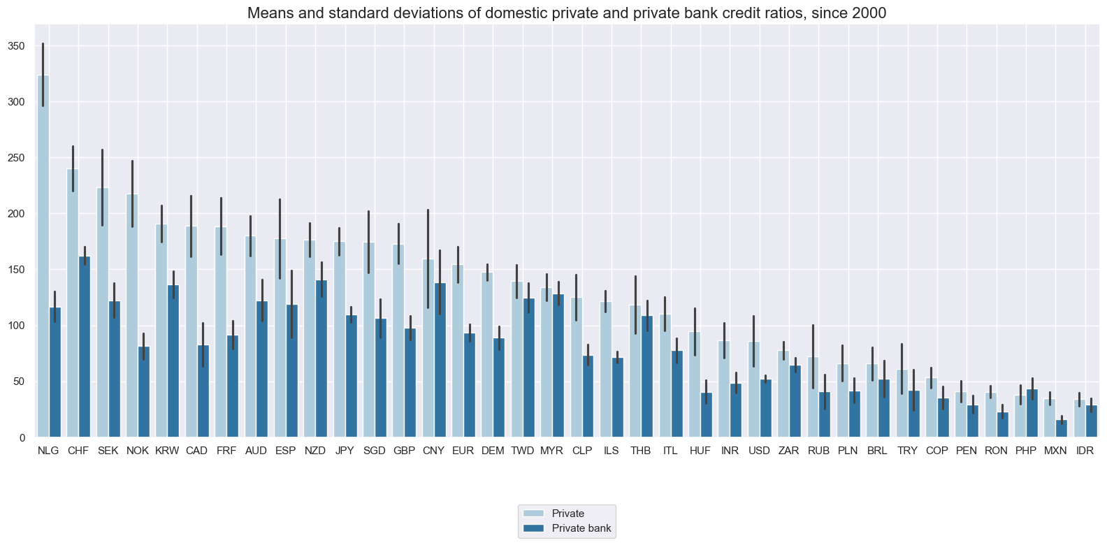
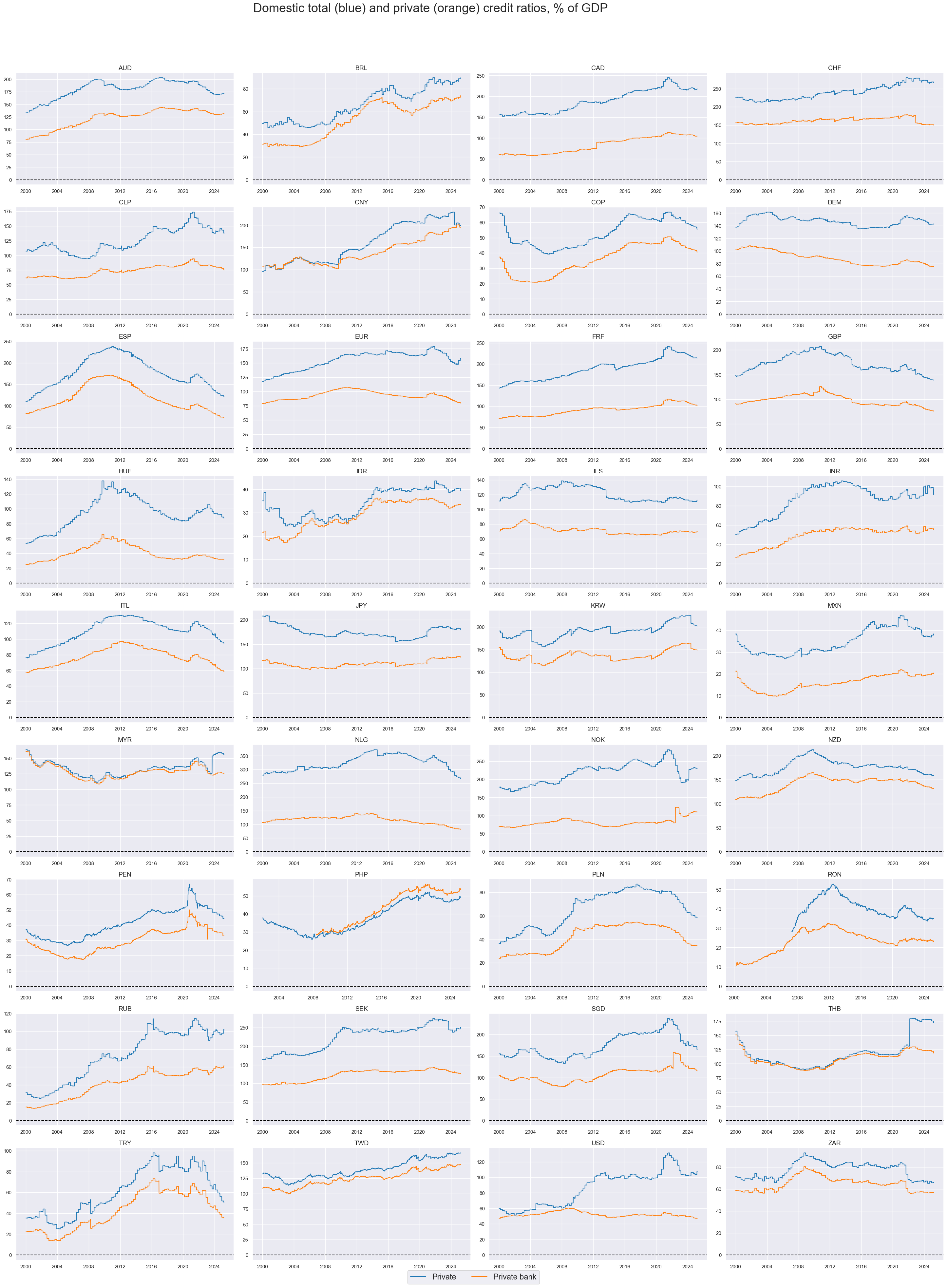
Across currency areas, bank credit ratios vary less than total credit ratios. The share of bank credit in total private credit has ranged from below 50% to 90% across countries. In some countries, like the U.S, the dynamics can be very different.

xcatx = ["DPCREDITGDP_NSA", "DPBCREDITGDP_NSA"]
cidx = cids_exp

msp.view_ranges(
    dfd,
    xcats=xcatx,
    cids=cidx,
    sort_cids_by="mean",
    start="2000-01-01",
    kind="bar",
    title="Means and standard deviations of domestic private and private bank credit ratios, since 2000",
    xcat_labels=["Private", "Private bank"],
    size=(16, 8),
)

xcatx = ["DPCREDITGDP_NSA", "DPBCREDITGDP_NSA"]
cidx = cids_exp

msp.view_timelines(
    dfd,
    xcats=xcatx,
    cids=cidx,
    start="2000-01-01",
    title="Domestic total (blue) and private (orange) credit ratios, % of GDP",
    xcat_labels=["Private", "Private bank"],
    title_adj=1.02,
    title_fontsize=27,
    legend_fontsize=17,
    title_xadj=0.455,
    label_adj=0.075,
    ncol=4,
    same_y=False,
    size=(12, 7),
    aspect=1.7,
    all_xticks=True,
)

Domestic debt securities ratios

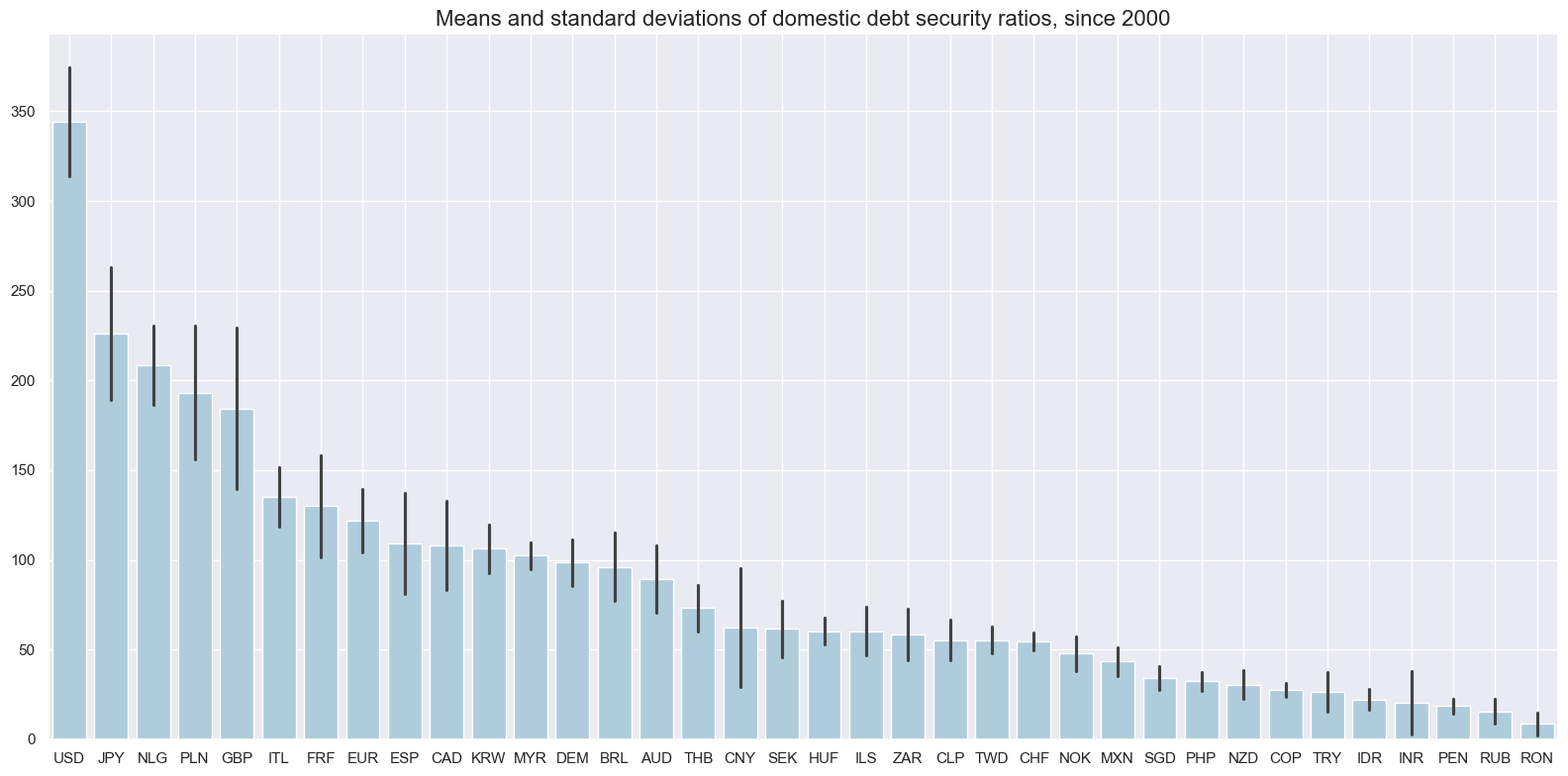
Ratios of debt securities to GDP are vastly different across currency areas, with the U.S. towering well above all other countries.

xcatx = ["DDEBTSECSGDP_NSA"]
cidx = cids_exp

msp.view_ranges(
    dfd,
    xcats=xcatx,
    cids=cidx,
    sort_cids_by="mean",
    title="Means and standard deviations of domestic debt security ratios, since 2000",
    start="2000-01-01",
    kind="bar",
    size=(16, 8),
)

xcatx = ["DDEBTSECSGDP_NSA"]
cidx = cids_exp

msp.view_timelines(
    dfd,
    xcats=xcatx,
    cids=cidx,
    start="2000-01-01",
    title="Domestic debt securities",
    title_adj=1.02,
    title_xadj=0.51,
    title_fontsize=27,
    legend_fontsize=17,
    ncol=4,
    same_y=False,
    size=(12, 7),
    aspect=1.7,
    all_xticks=True,
)

Importance

Research links

“A 145-year empirical analysis suggests that asset price surges are most dangerous when they are associated with rising financial leverage. The combination of housing price bubbles and credit booms has been the most detrimental of all.” Macrosynergy

Empirical clues

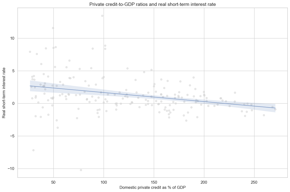
High credit ratios increase the stability risks arising from high or rising real interest rates. Hence, they often force policy makers to keep a lid on real interest rates. Historically, there has been a clear negative correlation between private credit ratios and real short-term interest rates.

cr_crr = msp.CategoryRelations(
    dfd,
    xcats=["DPCREDITGDP_NSA", "RIR_NSA"],
    cids=cids_exp,
    freq="M",
    lag=0,
    xcat_aggs=["mean", "mean"],
    start=start_date,
    years=5,
)
cr_crr.reg_scatter(
    title="Private credit-to-GDP ratios and real short-term interest rate",
    labels=False,
    ylab="Real short-term interest rate",
    xlab="Domestic private credit as % of GDP",
)

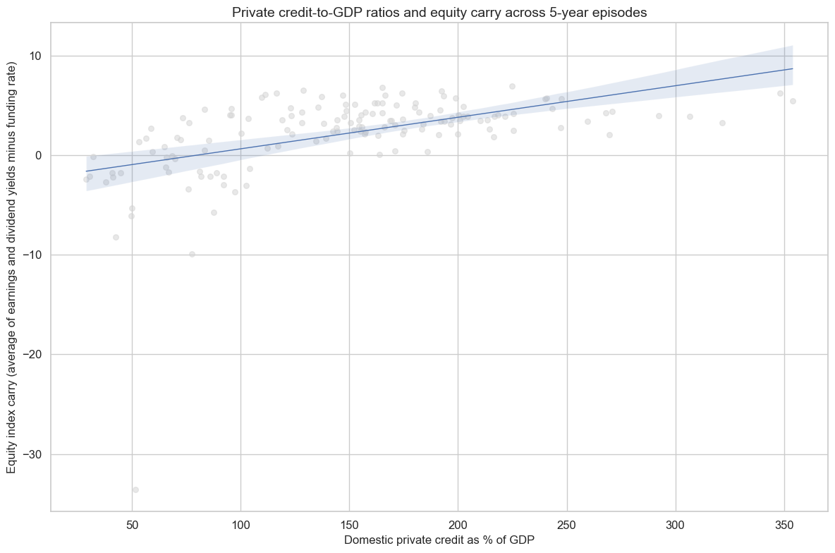
Partly as a result of the negative impact of credit ratios on real interest rates, there has been a strong positive correlation between credit ratios and equity “carry”, i.e. the differential between earnings or dividend yields and short-term funding costs.

cidx = list(
    set(cids_exp)
    - set(["CLP", "COP", "HUF", "IDR", "ILS", "NOK", "NZD", "PEN", "PHP", "RON", "RUB"])
)  # remove missing cids
cr_crr = msp.CategoryRelations(
    dfd,
    xcats=["DPCREDITGDP_NSA", "EQCRY_NSA"],
    cids=cidx,
    freq="M",
    lag=0,
    xcat_aggs=["mean", "mean"],
    start=start_date,
    years=5,
)
cr_crr.reg_scatter(
    title="Private credit-to-GDP ratios and equity carry across 5-year episodes",
    labels=False,
    ylab="Equity index carry (average of earnings and dividend yields minus funding rate)",
    xlab="Domestic private credit as % of GDP",
)

dfb = dfd[dfd["xcat"].isin(["FXTARGETED_NSA", "FXUNTRADABLE_NSA"])].loc[
    :, ["cid", "xcat", "real_date", "value"]
]
dfba = (
    dfb.groupby(["cid", "real_date"])
    .aggregate(value=pd.NamedAgg(column="value", aggfunc="max"))
    .reset_index()
)
dfba["xcat"] = "FXBLACK"
fxblack = msp.make_blacklist(
    dfba, "FXBLACK"
)  # exclude periods of FX targeting or illiquidity

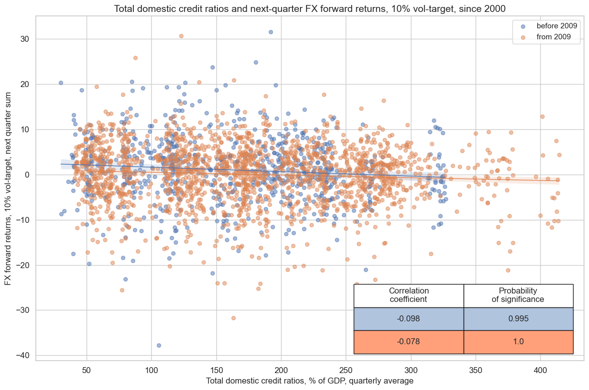
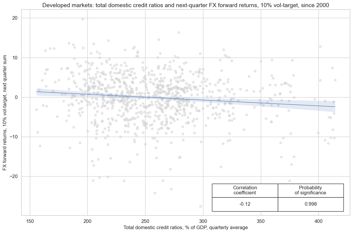
Historically, countries with higher domestic credit ratios have posted weaker FX returns than those with lower ratios. Indeed, domestic credit ratios would even have worked as a negative predictor. That may reflect that leveraged economies tend to have lower real interest rates and less scope for increasing rates in times of stress

cr = msp.CategoryRelations(
    dfd,
    xcats=["DCREDITGDP_NSA", "FXXR_VT10"],
    cids=list(set(cids_exp) - set(["USD"])),
    freq="Q",
    lag=1,
    xcat_aggs=["mean", "sum"],
    start="2000-01-01",
    blacklist=fxblack,
)
cr.reg_scatter(
    coef_box="lower right",
    prob_est="map",
    separator=2009,
    title="Total domestic credit ratios and next-quarter FX forward returns, 10% vol-target, since 2000",
    xlab="Total domestic credit ratios, % of GDP, quarterly average",
    ylab="FX forward returns, 10% vol-target, next quarter sum",
)

cr = msp.CategoryRelations(
    dfd,
    xcats=["DCREDITGDP_NSA", "FXXR_VT10"],
    cids=list(set(cids_dm) - set(["USD"])),
    freq="Q",
    lag=1,
    xcat_aggs=["mean", "sum"],
    start="2000-01-01",
    blacklist=fxblack,
)
cr.reg_scatter(
    coef_box="lower right",
    prob_est="map",
    title="Developed markets: total domestic credit ratios and next-quarter FX forward returns, 10% vol-target, since 2000",
    xlab="Total domestic credit ratios, % of GDP, quarterly average",
    ylab="FX forward returns, 10% vol-target, next quarter sum",
)

Appendices

Appendix 1: Currency symbols

The word ‘cross-section’ refers to currencies, currency areas or economic areas. In alphabetical order, these are AUD (Australian dollar), BRL (Brazilian real), CAD (Canadian dollar), CHF (Swiss franc), CLP (Chilean peso), CNY (Chinese yuan renminbi), COP (Colombian peso), CZK (Czech Republic koruna), DEM (German mark), ESP (Spanish peseta), EUR (Euro), FRF (French franc), GBP (British pound), HKD (Hong Kong dollar), HUF (Hungarian forint), IDR (Indonesian rupiah), ITL (Italian lira), JPY (Japanese yen), KRW (Korean won), MXN (Mexican peso), MYR (Malaysian ringgit), NLG (Dutch guilder), NOK (Norwegian krone), NZD (New Zealand dollar), PEN (Peruvian sol), PHP (Phillipine peso), PLN (Polish zloty), RON (Romanian leu), RUB (Russian ruble), SEK (Swedish krona), SGD (Singaporean dollar), THB (Thai baht), TRY (Turkish lira), TWD (Taiwanese dollar), USD (U.S. dollar), ZAR (South African rand).