Commodity future volatility #
This category group includes measures of realized return volatility for commodity futures. It also includes related generic leverage ratios for volatility targets.
Commodity future volatility #
Ticker : COXRxEASD_NSA
Label : Estimated annualized standard deviation of commodity future return.
Definition : Annualized standard deviation of commodity front future return, % of notional, based on exponential moving average of daily returns.
Notes :
-
The standard deviation has been calculated based on an exponential moving average of daily returns with a half-life of 11 active trading days.
-
The return is simply the % change in the front futures price. The return calculation assumes rolling futures (from front to second) on the first day of the month when the contract is due to expire. Not all commodities have monthly contracts.
-
For information on the components comprising each commodity group, see Appendix 1 .
Leverage ratio of vol-targeted commodity future position #
Ticker : COXRxLEV10_NSA
Label : Leverage ratio of commodity future position for 10% annualized vol target.
Definition : Commodity future leverage for a 10% annualized vol target, as ratio of contract notional relative to risk capital on which the return is calculated.
Notes :
-
This serves as the leverage ratio for a 10% annualized vol target and is inversely proportional to the estimated annualized standard deviation of the return on a USD1 notional position. The leverage can be viewed as indicative for positioning and endogenous market risk.
-
See also related important notes on “Commodity future volatility” (
COXRxEASD_NSA).
Imports #
Only the standard Python data science packages and the specialized
macrosynergy
package are needed.
import os
import numpy as np
import pandas as pd
import matplotlib.pyplot as plt
import seaborn as sns
import math

import json
import yaml

import macrosynergy.management as msm
import macrosynergy.panel as msp
import macrosynergy.signal as mss
import macrosynergy.pnl as msn


from macrosynergy.download import JPMaQSDownload

from timeit import default_timer as timer
from datetime import timedelta, date, datetime

import warnings

warnings.simplefilter("ignore")
The
JPMaQS
indicators we consider are downloaded using the J.P. Morgan Dataquery API interface within the
macrosynergy
package. This is done by specifying
ticker strings
, formed by appending an indicator category code
<category>
to a currency area code
<cross_section>
. These constitute the main part of a full quantamental indicator ticker, taking the form
DB(JPMAQS,<cross_section>_<category>,<info>)
, where
<info>
denotes the time series of information for the given cross-section and category. The following types of information are available:
-
valuegiving the latest available values for the indicator -
eop_lagreferring to days elapsed since the end of the observation period -
mop_lagreferring to the number of days elapsed since the mean observation period -
gradedenoting a grade of the observation, giving a metric of real time information quality.
After instantiating the
JPMaQSDownload
class within the
macrosynergy.download
module, one can use the
download(tickers,start_date,metrics)
method to easily download the necessary data, where
tickers
is an array of ticker strings,
start_date
is the first collection date to be considered and
metrics
is an array comprising the times series information to be downloaded.
cids_nfm = ["GLD", "SIV", "PAL", "PLT"]
cids_fme = ["ALM", "CPR", "LED", "NIC", "TIN", "ZNC"]
cids_ene = ["BRT", "WTI", "NGS", "GSO", "HOL"]
cids_sta = ["COR", "WHT", "SOY", "CTN"]
cids_liv = ["CAT", "HOG"]
cids_mis = ["CFE", "SGR", "NJO", "CLB"]

cids = cids_nfm + cids_fme + cids_ene + cids_sta + cids_liv + cids_mis
main = ["COXRxEASD_NSA", "COXRxLEV10_NSA"]
econ = []  # economic context
mark = ["COCRY_NSA", "COCRY_VT10", "COXR_NSA"]  # market links

xcats = main + econ + mark
# Download series from J.P. Morgan DataQuery by tickers

start_date = "1990-01-01"
tickers = [cid + "_" + xcat for cid in cids for xcat in xcats]
print(f"Maximum number of tickers is {len(tickers)}")

# Retrieve credentials

client_id: str = os.getenv("DQ_CLIENT_ID")
client_secret: str = os.getenv("DQ_CLIENT_SECRET")

# Download from DataQuery

with JPMaQSDownload(client_id=client_id, client_secret=client_secret) as downloader:
    start = timer()
    df = downloader.download(
        tickers=tickers,
        start_date=start_date,
        metrics=["value", "eop_lag", "mop_lag", "grading"],
        suppress_warning=True,
        show_progress=True,
    )
    end = timer()

dfd = df

print("Download time from DQ: " + str(timedelta(seconds=end - start)))
Maximum number of tickers is 125
Downloading data from JPMaQS.
Timestamp UTC:  2025-02-14 10:13:46
Connection successful!
Requesting data: 100%|█████████████████████████████████████████████████████████████████| 25/25 [00:05<00:00,  4.77it/s]
Downloading data: 100%|████████████████████████████████████████████████████████████████| 25/25 [00:25<00:00,  1.04s/it]
Some dates are missing from the downloaded data.
3 out of 9167 dates are missing.
Download time from DQ: 0:00:34.309351
Availability #
cids_exp = cids
msm.missing_in_df(dfd, xcats=main, cids=cids_exp)
No missing XCATs across DataFrame.
Missing cids for COXRxEASD_NSA:   []
Missing cids for COXRxLEV10_NSA:  []
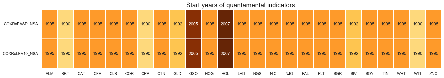
Most of commodities indicators are available from the early 1990s. Only a few energy products start in the 2000s: Brent, gasoline and natural gas.
For the explanation of currency symbols, which are related to currency areas or countries for which categories are available, please view Appendix 1 .
xcatx = main
cidx = cids_exp

dfx = msm.reduce_df(dfd, xcats=xcatx, cids=cidx)
dfs = msm.check_startyears(
    dfx,
)
msm.visual_paneldates(dfs, size=(20, 3))

print("Last updated:", date.today())
Last updated: 2025-02-14
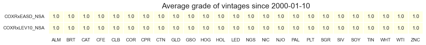
msp.heatmap_grades(dfd, xcats=main, cids=cids_exp, start="2000-01-10", size=(16, 1))
xcatx = main
msp.view_ranges(
dfd,
xcats=xcatx,
cids=cids_exp,
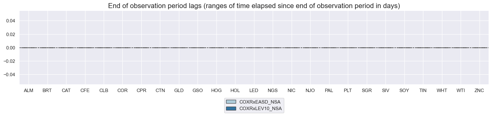
val="eop_lag",
title="End of observation period lags (ranges of time elapsed since end of observation period in days)",
start="2000-01-01",
kind="box",
size=(16, 4),
)
msp.view_ranges(
dfd,
xcats=xcatx,
cids=cids_exp,
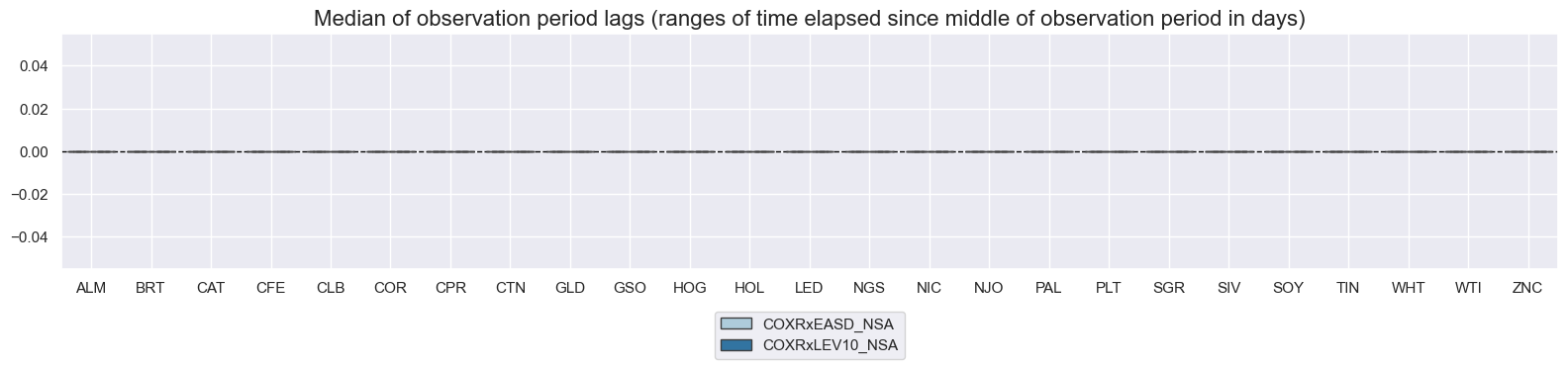
val="mop_lag",
title="Median of observation period lags (ranges of time elapsed since middle of observation period in days)",
start="2000-01-01",
kind="box",
size=(16, 4),
)
History #
Commodity future volatility #
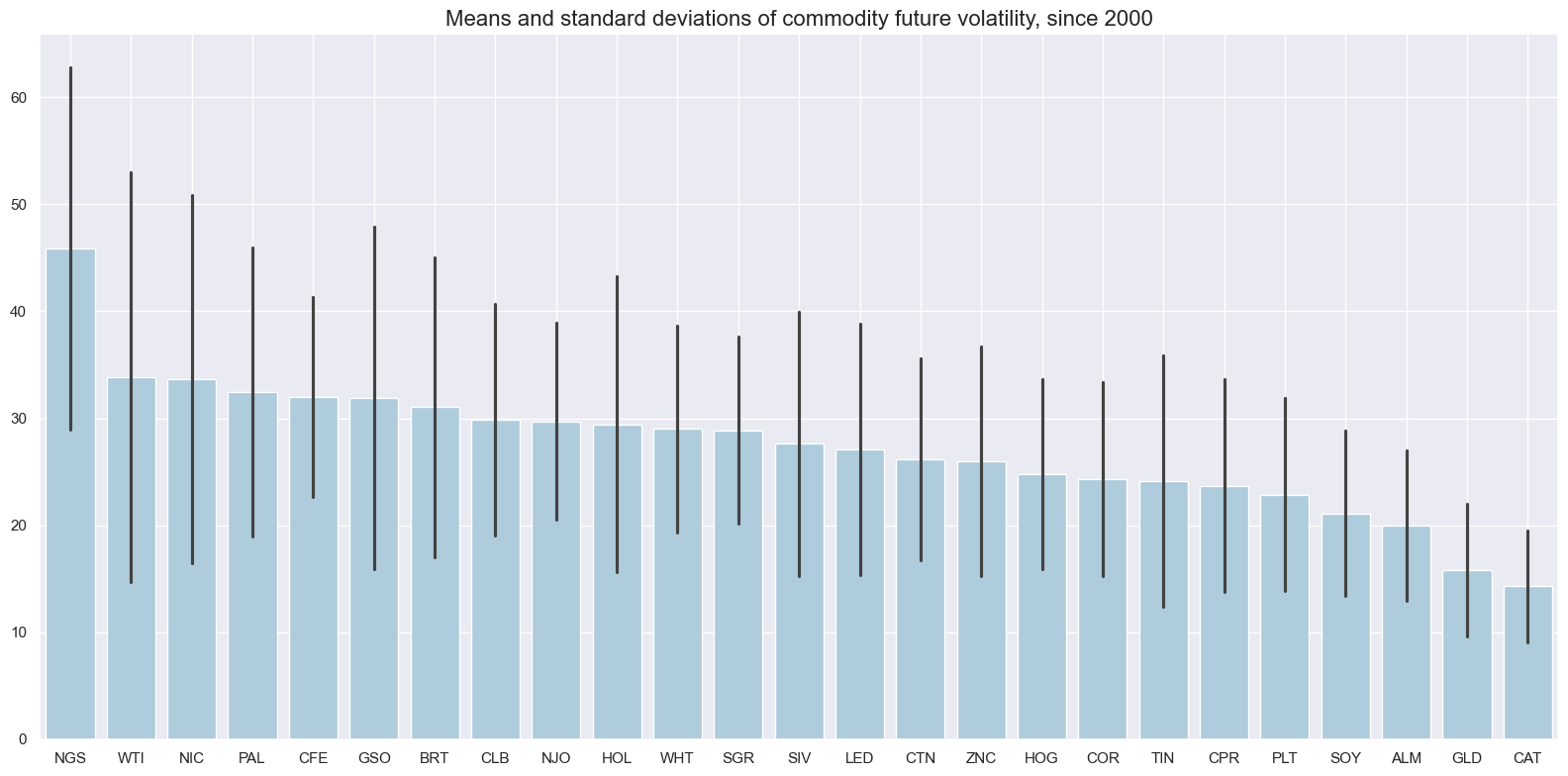
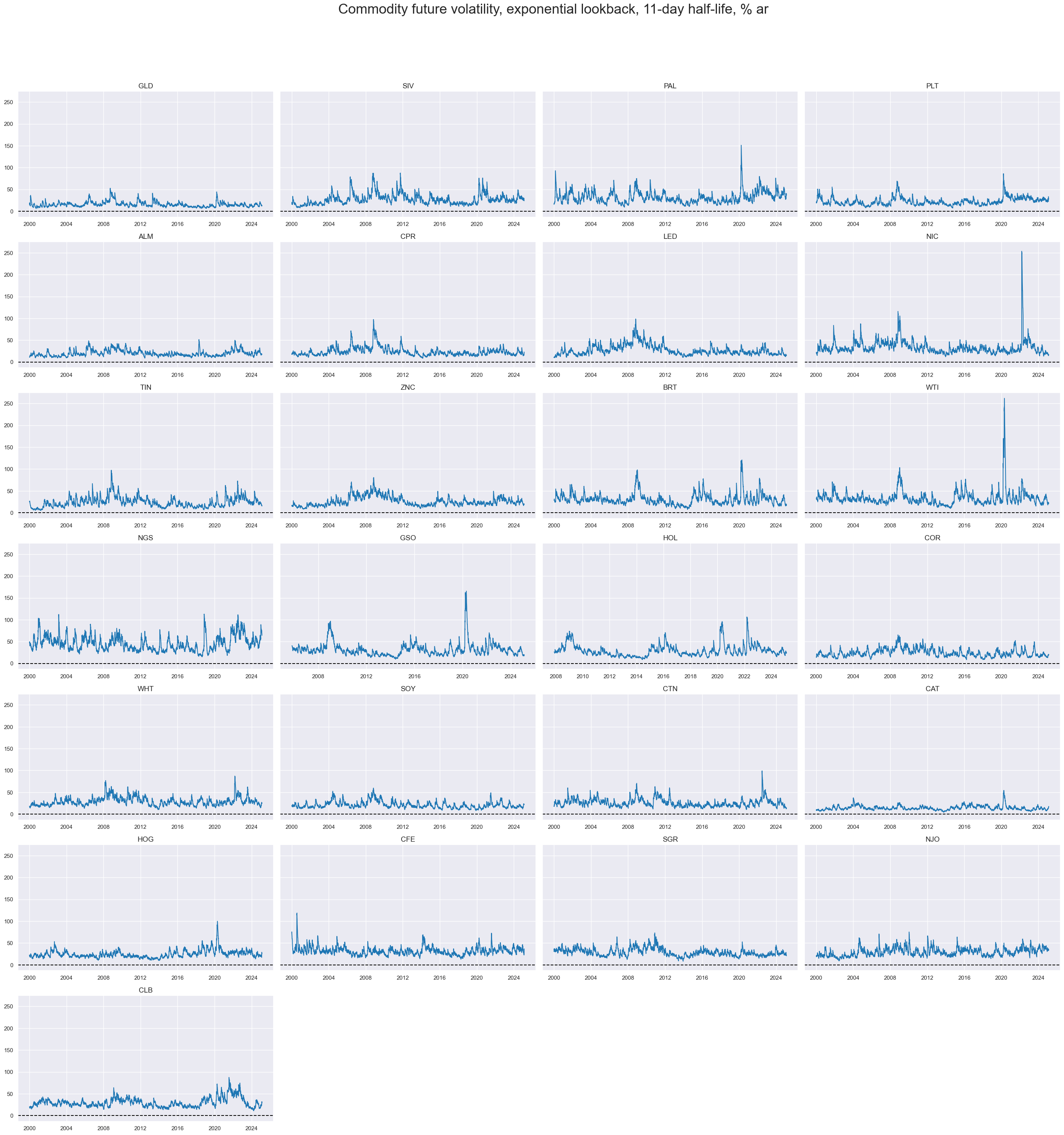
Average annualized volatility across commodities since 2000 ranges from over 40% (natural gas) to near 15% (live cattle). Spikes, i.e. large short-lived outliers, are discernible in many commodities.
xcatx = ["COXRxEASD_NSA"]
cidx = cids_exp

msp.view_ranges(
    dfd,
    xcats=xcatx,
    cids=cidx,
    sort_cids_by="mean",
    start="2000-01-01",
    title="Means and standard deviations of commodity future volatility, since 2000",
    kind="bar",
    size=(16, 8),
)
xcatx = ["COXRxEASD_NSA"]
cidx = cids_exp

msp.view_timelines(
    dfd,
    xcats=xcatx,
    cids=cidx,
    start="2000-01-01",
    title="Commodity future volatility, exponential lookback, 11-day half-life, % ar",
    title_adj=1.03,
    title_fontsize=27,
    title_xadj=0.52,
    cumsum=False,
    ncol=4,
    same_y=True,
    size=(12, 7),
    aspect=1.7,
    all_xticks=True,
)
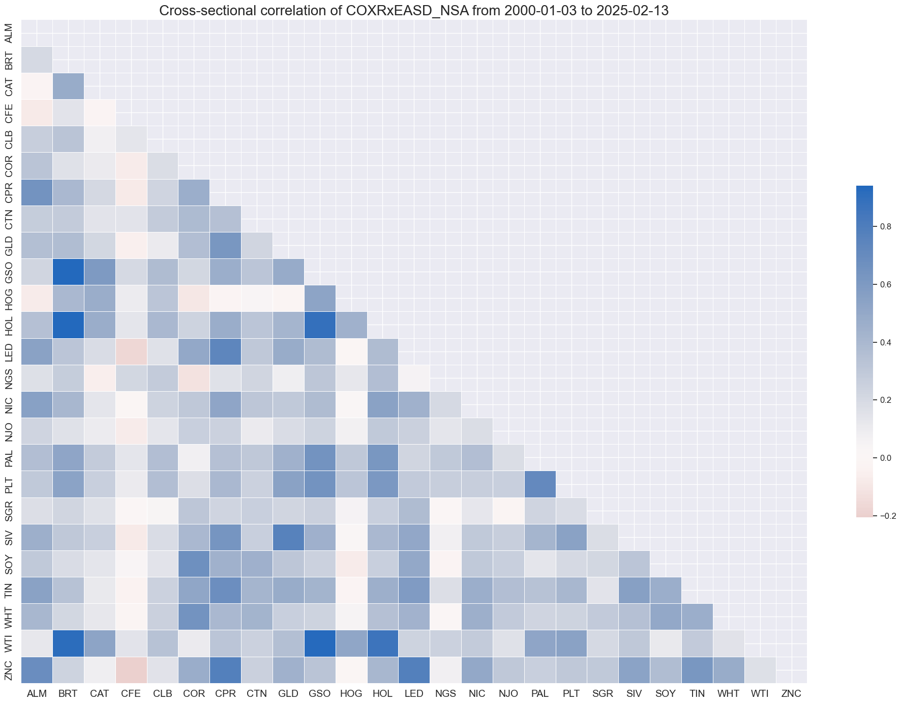
Realized volatility has mostly been positively correlated across commodities. But unlike in the equity space positive correlation has been quite weak and has not been universal. Coffee and livestock display little correlation with other commodities.
msp.correl_matrix(dfd, xcats="COXRxEASD_NSA", cids=cids_exp, size=(20, 14))
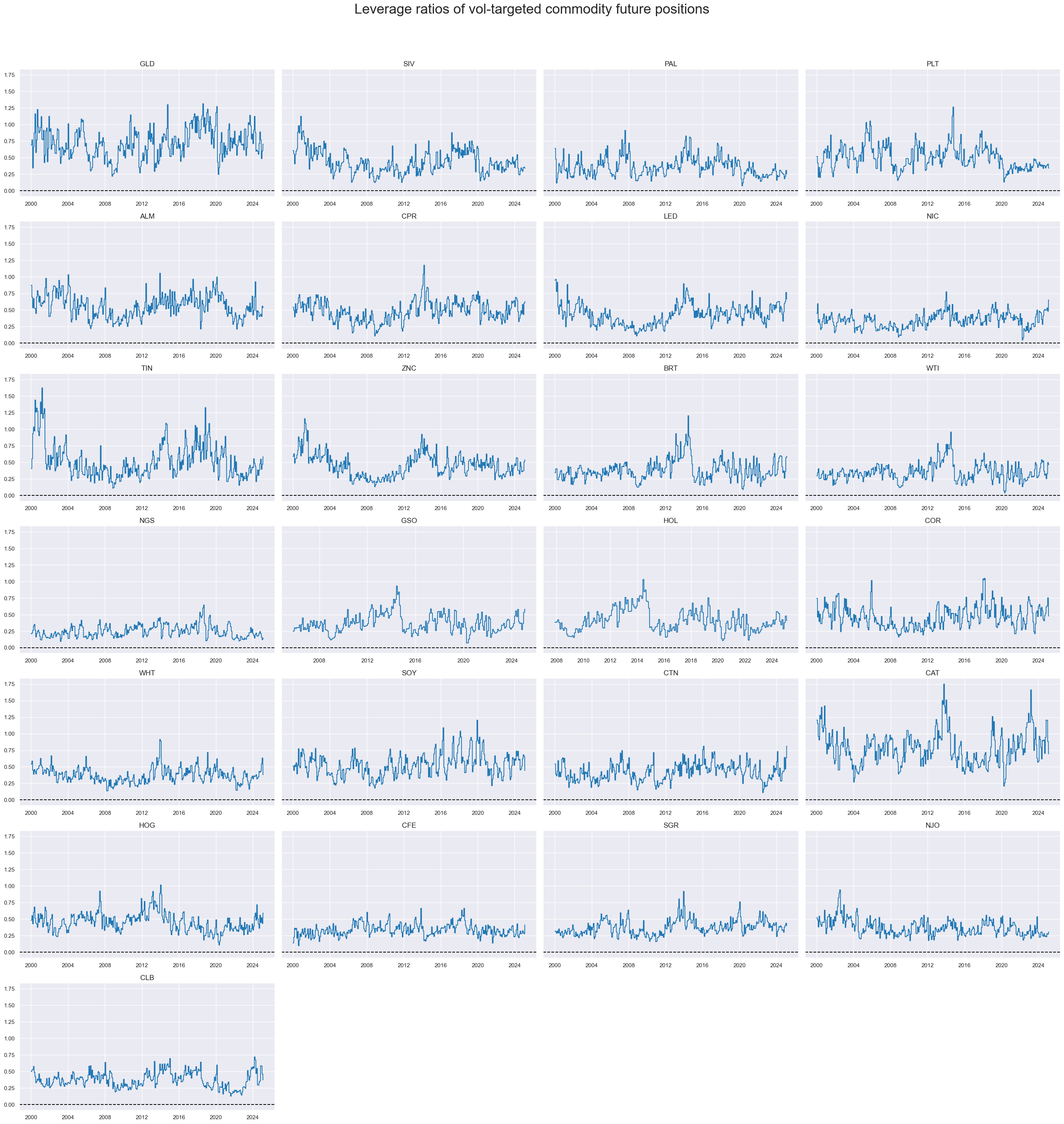
Leverage ratio of vol-targeted commodity future position #
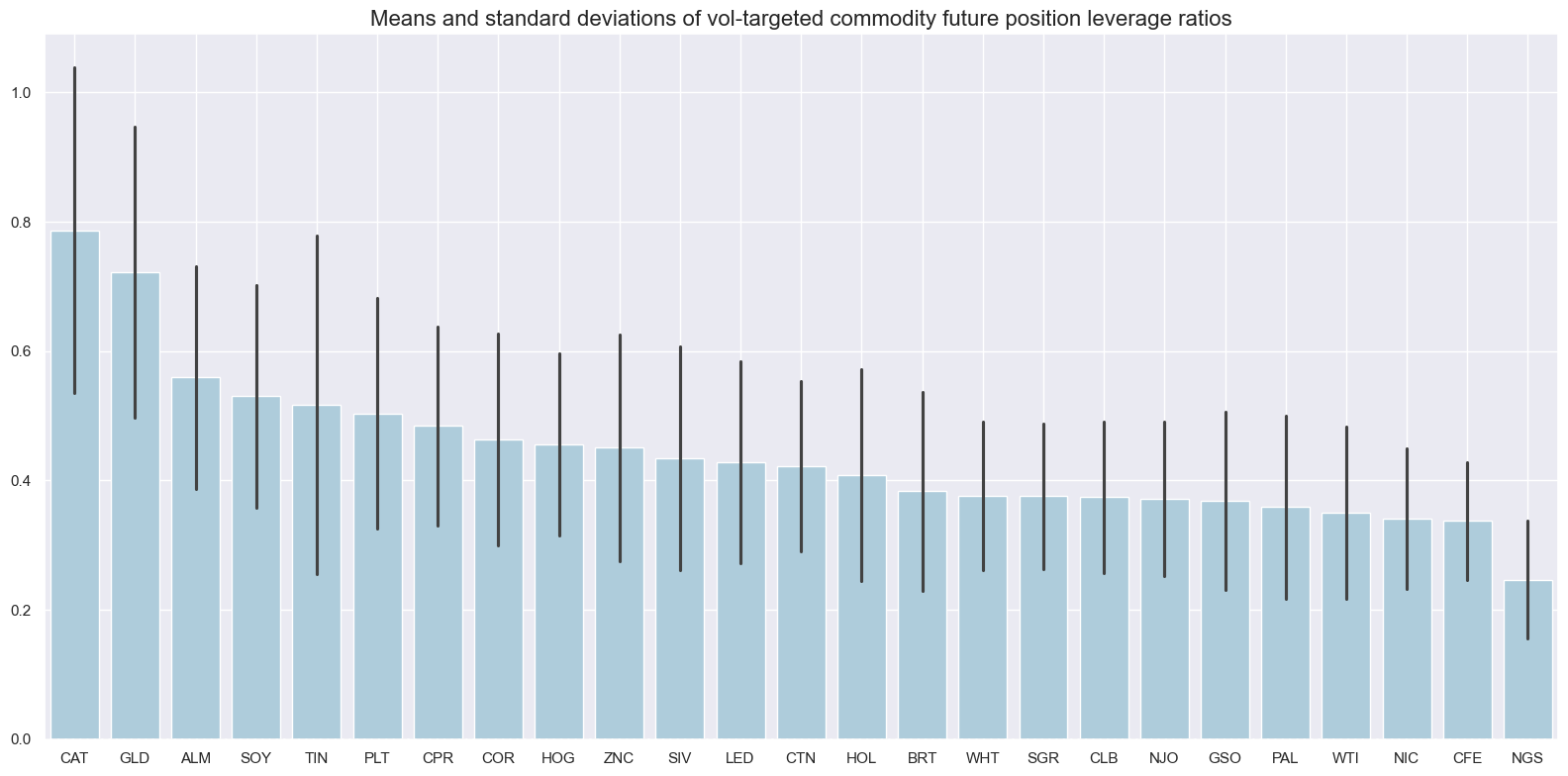
Since volatility of commodity returns is higher than for other asset clasess, leverage differences for equal volatility targets across markets have been low, between 0.2 and 0.75.
xcatx = ["COXRxLEV10_NSA"]
cidx = cids_exp
msp.view_ranges(
    dfd,
    xcats=xcatx,
    cids=cidx,
    sort_cids_by="mean",
    start="2000-01-01",
    title="Means and standard deviations of vol-targeted commodity future position leverage ratios",
    kind="bar",
    size=(16, 8),
)
xcatx = ["COXRxLEV10_NSA"]
cidx = cids_exp

msp.view_timelines(
    dfd,
    xcats=xcatx,
    cids=cidx,
    start="2000-01-01",
    title="Leverage ratios of vol-targeted commodity future positions",
    title_adj=1.02,
    title_fontsize=27,
    title_xadj=0.5,
    cumsum=False,
    ncol=4,
    same_y=True,
    size=(12, 7),
    aspect=1.7,
    all_xticks=True,
)
Importance #
Relevant research #
“Analysing volatility for the aggregate commodity market and for various commodity groups we find that factors associated with macroeconomic and financial market uncertainty explain subsequent volatility of commodity returns. Variables motivated by commodity pricing theories, such as the futures basis and hedging pressure, are also significant. Economic uncertainty measures based on differences in beliefs of economic agents extracted from survey data provide additional information to that contained in volatility series of current economic fundamentals. Finally, we find evidence of a strong bi-directional causal link between inflation uncertainty and commodity return volatility.” Prokopczuk and Symeonidis
“Volatility risk premia – differences between options-implied and actual volatility – are valid predictors for risky asset returns. High premia typically indicate high surcharges for the risk of changes in volatility, which are paid by investors with strong preference for more stable returns. For commodities volatility risk premia should have become a greater factor as consequence of their ‘financialization’. New evidence suggests that indeed volatility risk premia on commodity currencies have predictive power for subsequent commodity returns, while crude and gold premia have predictive power for other asset classes in accordance with the nature of these commodities. Since estimation of these premia takes some skill and judgment this points to opportunities for macro trading with econometric support” Macrosynergy
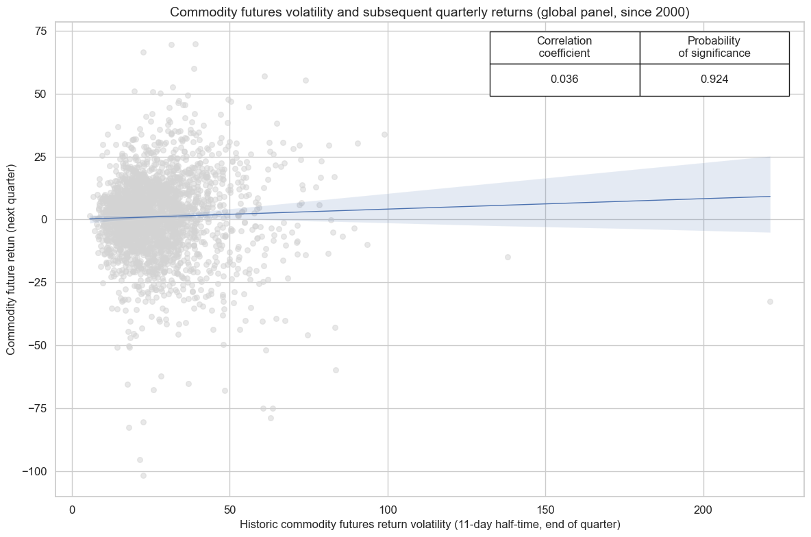
Empirical clues #
On balance, there has been a tendency for period and commodities with higher volatility leading higher returns.
cr = msp.CategoryRelations(
    dfd,
    xcats=["COXRxEASD_NSA", "COXR_NSA"],
    cids=cids_exp,
    freq="Q",
    lag=1,
    xcat_aggs=["last", "sum"],
    start="2000-01-01",
)
cr.reg_scatter(
    title="Commodity futures volatility and subsequent quarterly returns (global panel, since 2000)",
    labels=False,
    coef_box="upper right",
    xlab="Historic commodity futures return volatility (11-day half-time, end of quarter)",
    ylab="Commodity future retun (next quarter)",
)
Appendices #
Appendix 1: Commodity group definitions and symbols #
The commodity groups considered are: energy, base metals, precious metals, agricultural commodities and livestock.
-
The energy commodity group contains:
-
BRT : ICE Brent crude (IPE Brent crude before 2003)
-
WTI : NYMEX WTI light crude
-
NGS : NYMEX natural gas, Henry Hub
-
GSO : NYMEX RBOB Gasoline
-
HOL : NYMEX Heating oil, New York Harbor ULSD
-
-
The base metals group contains:
-
ALM : London Metal Exchange aluminium
-
CPR : Comex copper
-
LED : London Metal Exchange Lead
-
NIC : London Metal Exchange Nickel
-
TIN : London Metal Exchange Tin
-
ZNC : London Metal Exchange Zinc
-
-
The precious metals group contains:
-
GLD : COMEX gold 100 Ounce
-
SIV : COMEX silver 5000 Ounce
-
PAL : NYMEX palladium
-
PLT : NYMEX platinum
-
-
The agricultural commodity group contains:
-
COR : Chicago Board of Trade corn composite
-
WHT : Chicago Board of Trade wheat composite
-
SOY : Chicago Board of Trade soybeans composite
-
CTN : NYBOT / ICE cotton #2
-
CFE : NYBOT / ICE coffee ‘C’ Arabica
-
SGR : NYBOT / ICE raw cane sugar #11
-
NJO : NYBOT / NYCE FCOJ frozen orange juice concentrate
-
CLB : Chicago Mercantile Exchange random length lumber
-
-
The (U.S.) livestock commodity group contains:
-
CAT : Chicago Mercantile Exchange live cattle composite
-
HOG : Chicago Mercantile Exchange lean hogs composite
-