FX tail risk premia #
The category measures option-implied premia of the tail risk in FX forwards. The premium is calculated as the difference between the implied volatility of out-of-the-money options and at-the-money options, divided by the volatility of at-the-money options. A high ratio implies that the implied volatility of the out-of-the money option is larger and that buying protection against movements to the tail of return distribution is disproportionately expensive.
The out-of-the-money part of the ratio is based on 10-delta options. A 10-delta implied volatility is the implied volatility of an option that has roughly a 10% probability to be in the money. It is an option with a low likelihood of being exercised. There are two types of tail risk premium:
-
The downside tail risk premium is charged for the risk of large depreciation of the local currency versus the benchmark. It is calculated as the implied volatility of a 10-delta put (benchmark call) to the implied volatility of an at-the-money option of the same type.
-
The upside tail risk premium is charged for the risk of large appreciation of the local currency versus the benchmark. It is calculated as the ratio of implied volatility of a 10-delta call (benchmark put) to the implied volatility of an at-the-money option of the same type.
Imports #
Only the standard Python data science packages and the specialized
macrosynergy
package are needed.
import pandas as pd

import macrosynergy.management as msm
import macrosynergy.panel as msp
import macrosynergy.signal as mss
import macrosynergy.visuals as msv

from macrosynergy.download import JPMaQSDownload

from timeit import default_timer as timer
from datetime import timedelta, date
import os

import warnings

warnings.simplefilter("ignore")
The
JPMaQS
indicators we consider are downloaded using the J.P. Morgan Dataquery API interface within the
macrosynergy
package. This is done by specifying
ticker strings
, formed by appending an indicator category code
<category>
to a currency area code
<cross_section>
. These constitute the main part of a full quantamental indicator ticker, taking the form
DB(JPMAQS,<cross_section>_<category>,<info>)
, where
<info>
denotes the time series of information for the given cross-section and category. The following types of information are available:
-
valuegiving the latest available values for the indicator -
eop_lagreferring to days elapsed since the end of the observation period -
mop_lagreferring to the number of days elapsed since the mean observation period -
gradedenoting a grade of the observation, giving a metric of real time information quality.
After instantiating the
JPMaQSDownload
class within the
macrosynergy.download
module, one can use the
download(tickers,start_date,metrics)
method to easily download the necessary data, where
tickers
is an array of ticker strings,
start_date
is the first collection date to be considered and
metrics
is an array comprising the times series information to be downloaded.
cids_dmca = [
    "AUD",
    "CAD",
    "CHF",
    "EUR",
    "GBP",
    "JPY",
    "NOK",
    "NZD",
    "SEK",
    "USD",
]  # DM currency areas
cids_dmec = ["DEM", "ESP", "FRF", "ITL", "NLG"]  # DM euro area countries
cids_latm = ["BRL", "COP", "CLP", "MXN", "PEN"]  # Latam countries
cids_emea = ["CZK", "HUF", "ILS", "PLN", "RON", "RUB", "TRY", "ZAR"]  # EMEA countries
cids_emas = [
    "CNY",
    "HKD",
    "IDR",
    "INR",
    "KRW",
    "MYR",
    "PHP",
    "SGD",
    "THB",
    "TWD",
]  # EM Asia countries

cids_dm = cids_dmca + cids_dmec
cids_em = cids_latm + cids_emea + cids_emas
cids = sorted(cids_dm + cids_em)
main = [
    "FXPPTAILDOWN_NSA",
    "FXPPTAILUP_NSA",
    "FXPPTAILDOWNUSD_NSA",
    "FXPPTAILUPUSD_NSA",
]
econ = ["IVAWGT_SA_1YMA"]  # economic context

vols = ["EQXRxEASD_NSA", "FXXRxEASD_NSA", "DU10YXRxEASD_NSA", "CDS10YXRxEASD_NSA"]

mark = ["EQXR_NSA",
    "EQXR_VT10",
    "FXXR_NSA",
    "FXXR_VT10",
    "FXTARGETED_NSA",
    "FXUNTRADABLE_NSA",
    "CDS10YXR_NSA",
    "CDS10YXR_VT10",
    "LCBIR_NSA",
    "FCBIR_NSA"]  # market links

xcats = main + econ + mark + vols

cids_co = ["GLD"]  # gold
xcats_co = ["COXR_VT10", "COXR_NSA"]  # Commodity future returns

tix_co = [c + "_" + x for c in cids_co for x in xcats_co]
# Download series from J.P. Morgan DataQuery by tickers

start_date = "2000-01-01"
tickers = [cid + "_" + xcat for cid in cids for xcat in xcats] + tix_co
print(f"Maximum number of tickers is {len(tickers)}")

# Retrieve credentials

client_id: str = os.getenv("DQ_CLIENT_ID")
client_secret: str = os.getenv("DQ_CLIENT_SECRET")

# Download from DataQuery

with JPMaQSDownload(client_id=client_id, client_secret=client_secret) as downloader:
    start = timer()
    assert downloader.check_connection()
    df = downloader.download(
        tickers=tickers,
        start_date=start_date,
        metrics=["value", "eop_lag", "mop_lag", "grading"],
        suppress_warning=True,
    )
    end = timer()

dfd = df

print("Download time from DQ: " + str(timedelta(seconds=end - start)))
Maximum number of tickers is 724
Downloading data from JPMaQS.
Timestamp UTC:  2025-06-25 10:49:34
Connection successful!
Some expressions are missing from the downloaded data. Check logger output for complete list.
684 out of 2896 expressions are missing. To download the catalogue of all available expressions and filter the unavailable expressions, set `get_catalogue=True` in the call to `JPMaQSDownload.download()`.
Download time from DQ: 0:01:04.337442
Availability #
cids_exp = sorted(
    list(set(cids) - set(cids_dmec) - set(["HKD"]))
)  # cids expected in category panels
msm.missing_in_df(dfd, xcats=main, cids=cids_exp)
No missing XCATs across DataFrame.
Missing cids for FXPPTAILDOWNUSD_NSA:  ['USD']
Missing cids for FXPPTAILDOWN_NSA:     ['USD']
Missing cids for FXPPTAILUPUSD_NSA:    ['USD']
Missing cids for FXPPTAILUP_NSA:       ['USD']
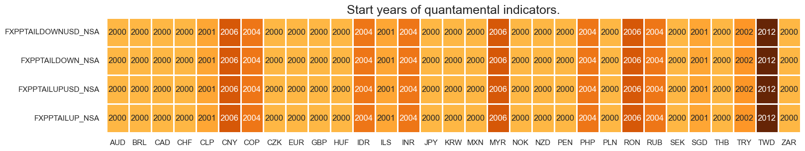
Whilst most quantamental indicators of FX tail risk premia are available from 2000, including all those for developed markets, some emerging market series’ are only available from the mid-2000s onwards.
For the explanation of currency symbols, which are related to currency areas or countries for which categories are available, please view Appendix 1 .
xcatx = main
cidx = cids_exp

dfx = msm.reduce_df(dfd, xcats=xcatx, cids=cidx)
dfs = msm.check_startyears(
    dfx,
)
msm.visual_paneldates(dfs, size=(18, 3))

print("Last updated:", date.today())
Last updated: 2025-06-25
History #
FX tail risk premium against dominant benchmark #
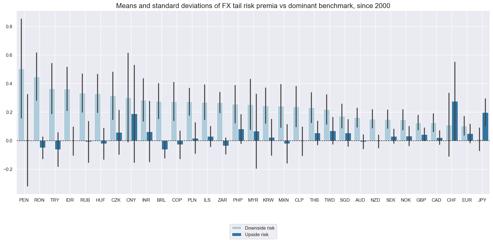
Downside risk premia have on average been positive for all non-USD currencies since 2000. They have been the largest in some EM currencies with historically low spot-exchange rate volatility in normal times, such as Peru and Romania. This is likely related to the risk of breaks in managed FX regimes. Upside risk premia have been more balanced and closer to zero, with the notable exceptions of CHF, JPY and CNY. CHF, JPY and GBP have been the oly currencies with higher average upside risk premia and downside risk premia.
xcatx = ["FXPPTAILDOWN_NSA", "FXPPTAILUP_NSA"]
cidx = cids_exp

msp.view_ranges(
    dfd,
    xcats=xcatx,
    cids=cidx,
    sort_cids_by="mean",
    start=start_date,
    title="Means and standard deviations of FX tail risk premia vs dominant benchmark, since 2000",
    xcat_labels=["Downside risk", "Upside risk"],
    kind="bar",
    size=(16, 8),
)
xcatx = ["FXPPTAILDOWN_NSA", "FXPPTAILUP_NSA"]
cidx = cids_exp
msp.view_timelines(
dfd,
xcats=xcatx,
cids=cidx,
start=start_date,
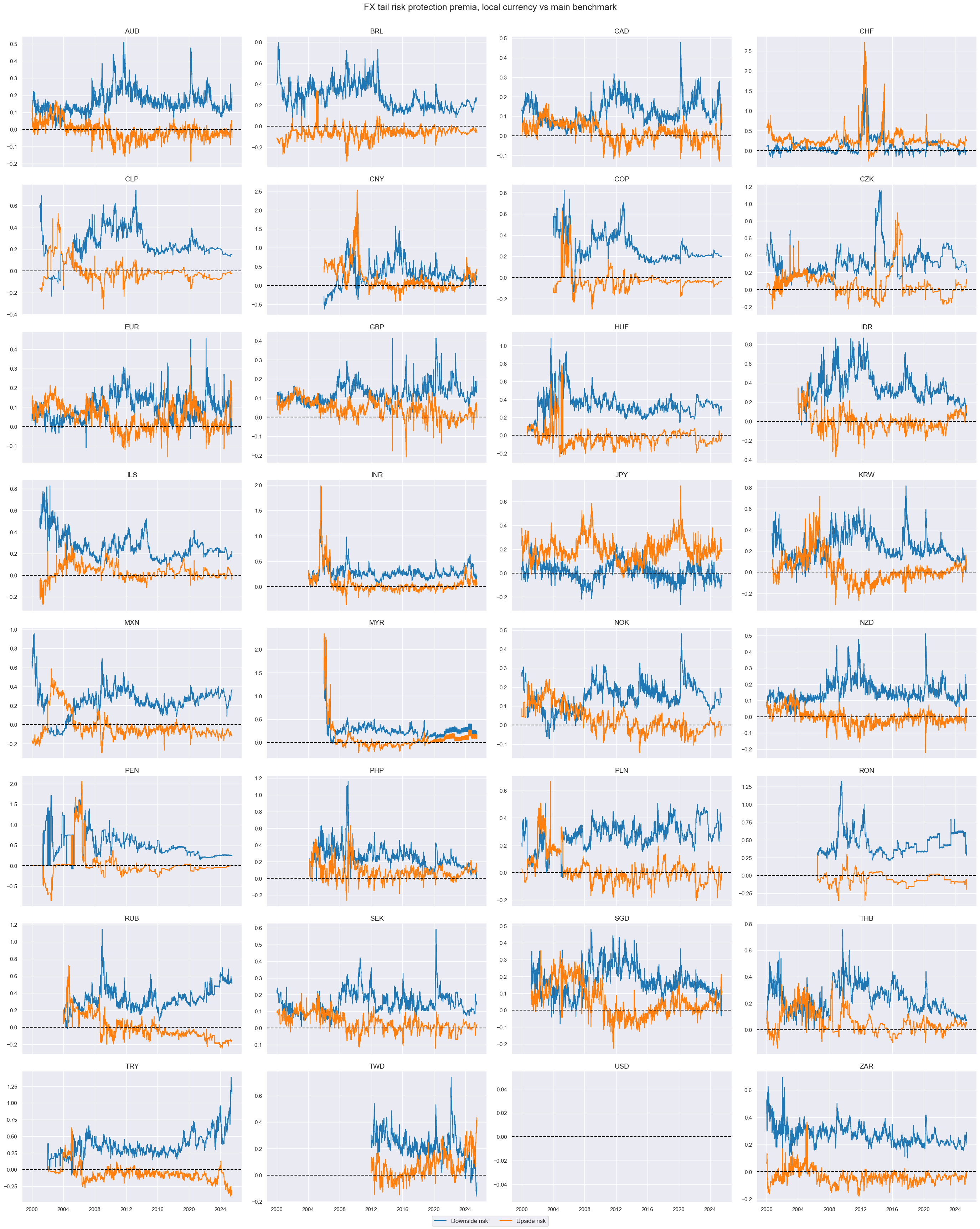
title="FX tail risk protection premia, local currency vs main benchmark",
xcat_labels=["Downside risk", "Upside risk"],
ncol=4,
same_y=False,
)
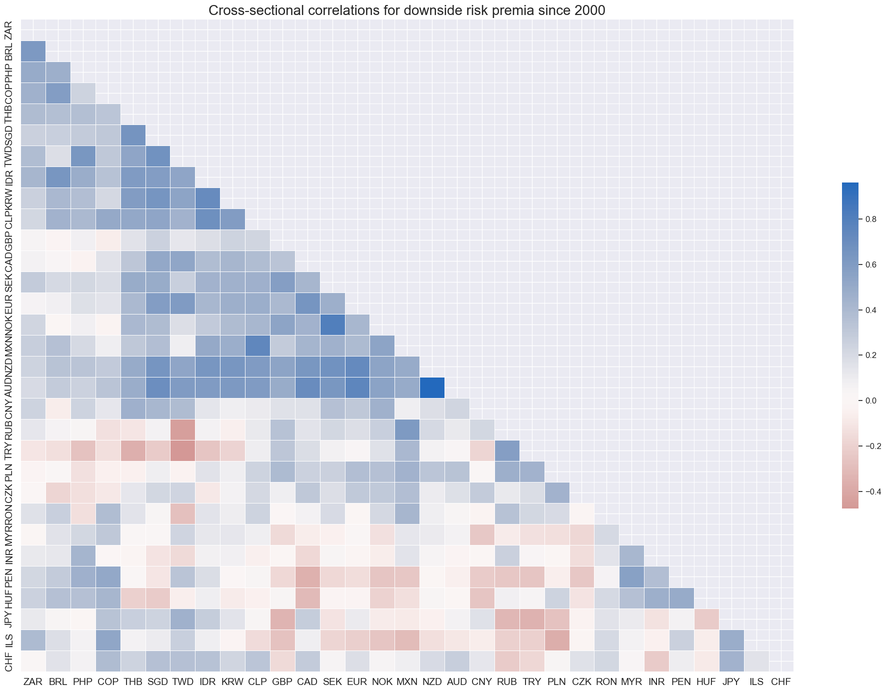
Downside risk premia have been positively correlated across most exchange rate pairs.
xcatx = "FXPPTAILDOWN_NSA"
cidx = cids_exp

dfd_vrp7 = dfd[dfd["xcat"] == "FXPPTAILDOWN_NSA"][
    ["real_date", "cid", "xcat", "value"]
].set_index("real_date")
dfw_vrp7 = dfd_vrp7.groupby(["cid", "xcat"]).resample("M").mean().reset_index()
msp.correl_matrix(
    dfw_vrp7,
    xcats=xcatx,
    cids=cidx,
    size=(20, 14),
    title="Cross-sectional correlations for downside risk premia since 2000",
    cluster=True,
)
FX tail risk premium against USD #
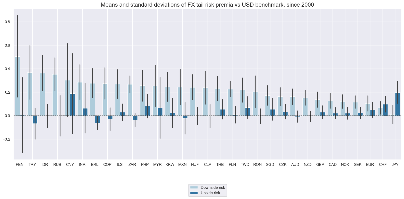
As for dominant benchmarks, downside tail risk premia have been positive for all currencies against the USD.
xcatx = ["FXPPTAILDOWNUSD_NSA", "FXPPTAILUPUSD_NSA"]
cidx = cids_exp

msp.view_ranges(
    dfd,
    xcats=xcatx,
    cids=cidx,
    sort_cids_by="mean",
    start=start_date,
    title="Means and standard deviations of FX tail risk premia vs USD benchmark, since 2000",
    xcat_labels=["Downside risk", "Upside risk"],
    kind="bar",
    size=(16, 8),
)
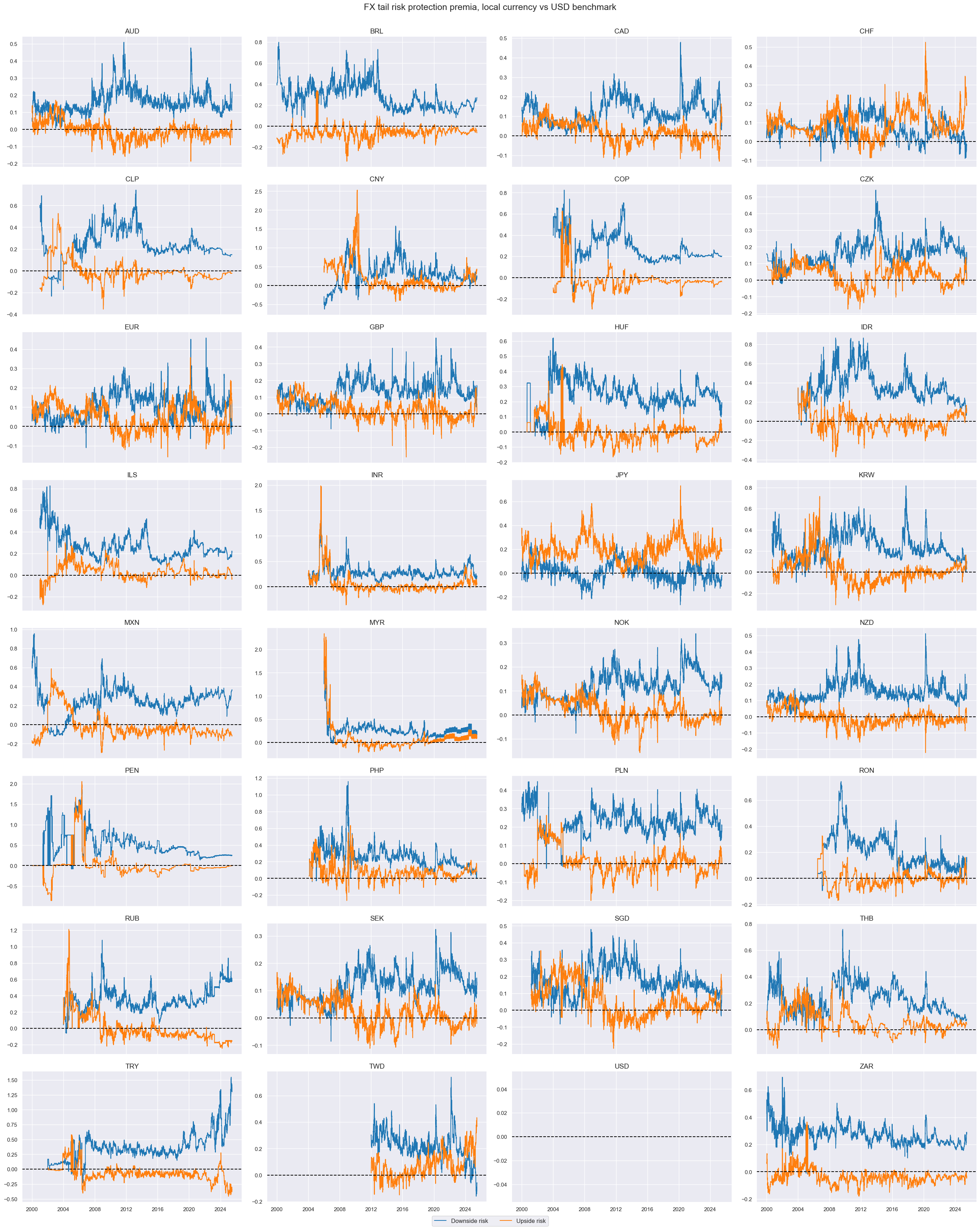
xcatx = ["FXPPTAILDOWNUSD_NSA", "FXPPTAILUPUSD_NSA"]
cidx = cids_exp

msp.view_timelines(
    dfd,
    xcats=xcatx,
    cids=cidx,
    start=start_date,
    title="FX tail risk protection premia, local currency vs USD benchmark",
    xcat_labels=["Downside risk", "Upside risk"],
    ncol=4,
    same_y=False,
    all_xticks=False,
)
Importance #
Research Links #
“One of the pillars of modern finance theory is the concept of ‘risk premium’, i.e. that a more risky investment should, on the long run, also be more profitable.” Lempérière, et al.
“(FX) tail risk is mostly influenced by the long position of the carry trade… Historically, Carry trades have been a success story for most investors and a major source of funds for emerging economies maintaining higher interest rates.” Ganepola
“We propose a new decomposition of the variance risk premium in terms of upside and downside variance risk premia. These components reflect market compensation for changes in good and bad uncertainties. Their difference is a measure of skewness risk premium, which captures investors’ asymmetric views on favorable versus undesirable risks.” Feunou, Jahan-Parvar, Okou
“… this paper proposes and empirically shows that the two seemingly unrelated markets, sovereign credit and far-out-of-the-money (FOM) FX options, are related by no-arbitrage because they share the same tail risk. “ Georgievska
“… we show that much of this predictability (future market returns) may be attributed to time variation in the part of the variance risk premium associated with the special compensation demanded by investors for bearing jump tail risk, consistent with the idea that market fears play an important role in understanding the return predictability.” Bollerslev, Todorov & Xu
“Developed economies have higher inward and outward tail risk spillovers than developing economies.” He, Yu, Luo & Yan
“We show that the currency volatility risk premium has substantial predictive power for the cross-section of currency returns. Currencies with low implied volatility relative to historical realized volatility those with relatively cheap volatility insurance predictably appreciate, while currencies with relatively more expensive volatility insurance predictably depreciate.” Della Corte, et al.
Empirical Clues #
Before running further analysis, we exclude periods when FX markets had limited tradability. We then normalize the relevant time series using the make_zn_scores() function, which centers the data around a neutral reference point (such as the mean of the whole panel or the mean of particular cross-section). A zn-score indicates how far a value deviates from this reference, scaled by a selected spread measure (e.g., standard deviation).
dfb = dfd[dfd["xcat"].isin(["FXTARGETED_NSA", "FXUNTRADABLE_NSA"])].loc[
    :, ["cid", "xcat", "real_date", "value"]
]
dfba = (
    dfb.groupby(["cid", "real_date"])
    .aggregate(value=pd.NamedAgg(column="value", aggfunc="max"))
    .reset_index()
)
dfba["xcat"] = "FXBLACK"
fxblack = msp.make_blacklist(dfba, "FXBLACK")

dfx=dfd.copy()
xcatx = main + vols

zn_variants = [
    {"postfix": "PZ", "pan_weight": 1},
    {"postfix": "IZ", "pan_weight": 0},
]

for xcat in xcatx:
    for variant in zn_variants:
        dfa = msp.make_zn_scores(
            dfx,
            xcat=xcat,
            cids=cids,
            neutral="mean",
            sequential=True,
            min_obs=261 * 3,
            pan_weight=variant["pan_weight"],
            thresh=3,
            postfix=variant["postfix"],
            est_freq="m",
        )
        dfx = msm.update_df(dfx, dfa)
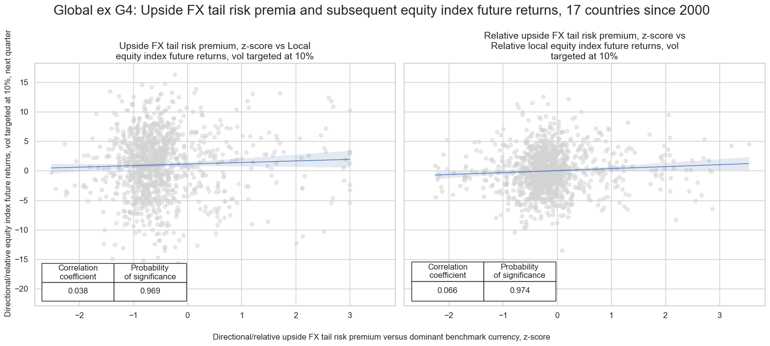
FX tail risk premium and subsequent equity index future returns #
All other things equal, upside FX risk in smaller economies (all excluding U.S., euro area, Japan and China) should translate into downside risk of local-currency prices of equity, as a large part of corporate revenues come from abroad. This risk should command a premium. Indeed, upside FX tail risk premia have been positively related to subsequent local-currency equity index future returns. The predictive relation has been significant at both a monthly and quarterly frequency. There has been an even stronger positive relation between relative upside tail risk premia and subsequent relative equity index returns.
cids_dm_small = ["AUD", "CAD", "CHF", "NOK", "SEK"]
cids_glb = cids_em + cids_dm_small

# Define region-specific settings
regions = {
    "vEM": cids_em,
    "vGLB": cids_glb
}

xcatx = ["EQXR_NSA", "EQXR_VT10", "FXPPTAILUP_NSAPZ"]

# Loop through regions and generate relative value xcats
for postfix, cids_group in regions.items():
    dfa = msp.make_relative_value(
        dfx,
        xcats=xcatx,
        cids=cids_group,
        start="2000-01-01",
        rel_meth="subtract",
        complete_cross=False,
        postfix=postfix,
    )
    dfx = msm.update_df(dfx, dfa)
# Define signal and target mappings
sigx = {
    "FXPPTAILUP_NSAPZ": "Upside FX tail risk premium, z-score",
    "FXPPTAILUP_NSAPZvGLB": "Relative upside FX tail risk premium, z-score"
}

targx = {
    "EQXR_VT10": "Local equity index future returns, vol targeted at 10%",
    "EQXR_VT10vGLB": "Relative local equity index future returns, vol targeted at 10%"
}

# Pair signals and targets one-to-one
paired_sig_targ = list(zip(sigx.keys(), targx.keys()))

# Get common cross-section identifiers
cidx = msm.common_cids(dfx, xcats=list(sigx.keys()) + list(targx.keys()))
cidx = list(set(cidx) & set(cids_glb))

# Run CategoryRelations and store
cr = {}
for sig_name, targ_name in paired_sig_targ:
    key = f"cr_{targ_name}_{sig_name}"
    cr[key] = msp.CategoryRelations(
        dfx,
        xcats=[sig_name, targ_name],
        cids=cidx,
        freq="Q",
        lag=1,
        xcat_aggs=["last", "sum"],
        blacklist=fxblack,
        start="2000-01-01",
    )

# Gather all CategoryRelations
all_cr_instances = list(cr.values())

# Prepare subplot titles
subplot_titles = [
    f"{sigx[sig_key]} vs {targx[targ_key]}"
    for sig_key, targ_key in paired_sig_targ
]

# Get suffix from target descriptions
common_suffix = list(targx.values())[0].split(" ", 1)[1]

msv.multiple_reg_scatter(
    all_cr_instances,
    title=f"Global ex G4: Upside FX tail risk premia and subsequent equity index future returns, {len(cidx)} countries since 2000",
    xlab="Directional/relative upside FX tail risk premium versus dominant benchmark currency, z-score",
    ylab=f"Directional/relative {common_suffix}, next quarter",
    ncol=2,
    nrow=1,
    figsize=(16, 7),
    prob_est="map",
    subplot_titles=subplot_titles,
    coef_box="lower left",
)
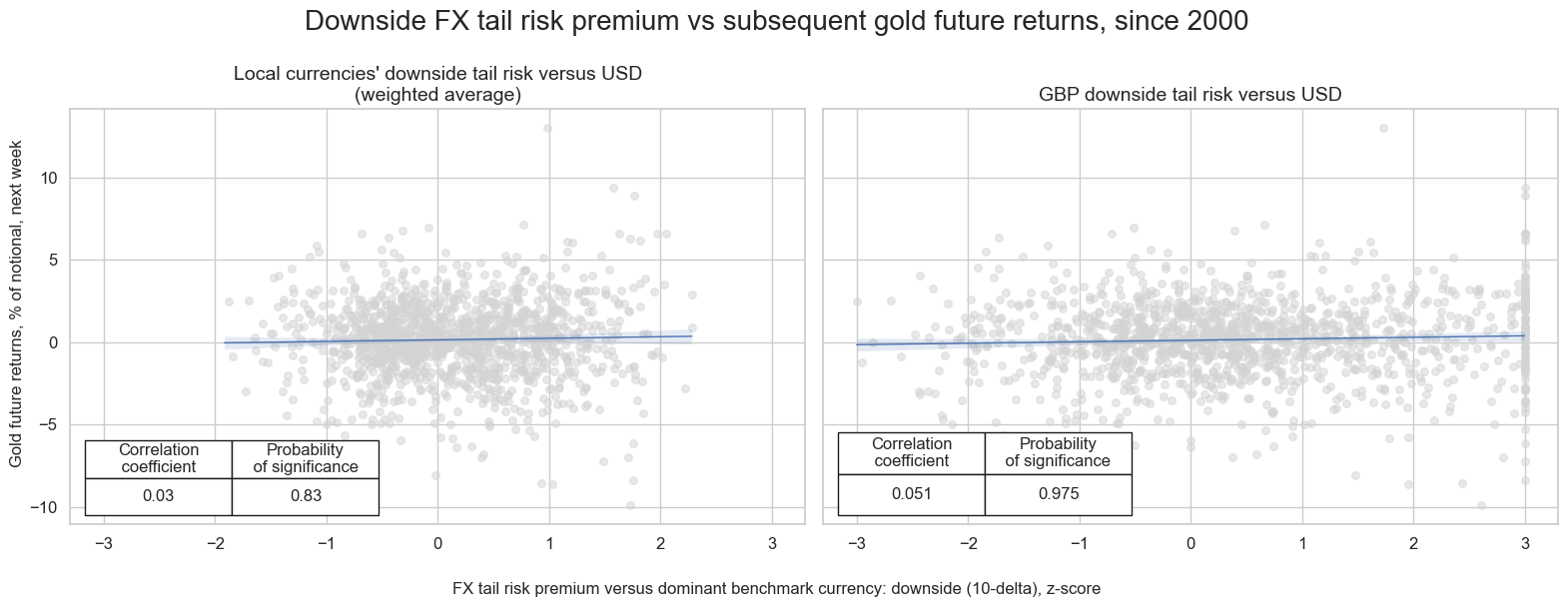
FX tail risk premia versus the USD and gold returns #
FX tail risk premia on various currencies vis-a-vis the dollar imply tail risk premia on gold as well. First, gold futures are denominated in dollars and its sharp appreciation would naturally weigh on the dollar price of international commodities. Second, sharpe dollar appreciation can put stress on dollar funding, another tail risk that would affect commodities in general and gold in particular.
# Step 1: Filter for Gold-related commodity returns
gold_cats = ["COXR_VT10", "COXR_NSA"]
dfx_gld = dfx[dfx["xcat"].isin(gold_cats) & (dfx["cid"] == "GLD")]

# Step 2: Define the indicators and currencies to map to the gold cross-section
xcatx = ["FXPPTAILDOWNUSD_NSAIZ", "IVAWGT_SA_1YMA"]
#currencies = ["EUR", "GBP", "CHF"]
currencies = cids

# Step 3: Loop through each currency, align it to gold's cross-section, and update the result
dfx_gold = dfx_gld.copy()

for cid in currencies:
    df_curr = dfx[(dfx["xcat"].isin(xcatx)) & (dfx["cid"] == cid)]
    df_curr = msm.update_df(dfx_gld, df_curr)
    df_curr["cid"] = cid
    dfx_gold = msm.update_df(dfx_gold, df_curr)

# Step 4: Create a composite cross-section for the downside weighted with respective Share in world GDP (USD terms): based on 1-year moving average
composite_cid = "Weighted local currency tail risk vis-a-vis USD"

dflc = msp.linear_composite(
    df=dfx,
    xcats="FXPPTAILDOWNUSD_NSAIZ",
    cids=currencies,
    weights="IVAWGT_SA_1YMA",
    normalize_weights=True,
    complete_cids=False,
    new_cid=composite_cid,
)

dflc = msm.update_df(dfx_gld, dflc)
dfx_gold = msm.update_df(dfx_gold, dflc)

# Copy COXR_NSA for GLD and assign to new cid
df_copy = dfx[(dfx["xcat"].isin(["COXR_NSA", "COXR_VT10"])) & (dfx["cid"] == "GLD")].copy()
df_copy["cid"] = composite_cid

# Update main DataFrame with the copied data
dfx_gold = msm.update_df(dfx_gold, df_copy)
Positive predictive power of the US dollar upside risk premium for Gold returns holds on daily, weekly, and monthly frequencies. This relationship is particularly strong for USD/GBP downside risk.
sigx = {
    "FXPPTAILDOWNUSD_NSAIZ": "FX tail risk premium versus dominant benchmark currency: downside (10-delta), z-score"
}

targx = {
    "COXR_NSA": "Gold future returns, % of notional",
}


# --- Common Parameters ---
xcats = list(sigx.keys()) + list(targx.keys())
common_kwargs = {
    "df": dfx_gold,
    "xcats": xcats,
    "freq": "W",
    "lag": 1,
    "xcat_aggs": ["last", "sum"],
    "start": "2000-01-01",
}

# --- Create CategoryRelations Objects ---
cr_comp = msp.CategoryRelations(
    cids=["Weighted local currency tail risk vis-a-vis USD"], **common_kwargs
)
cr_gbp = msp.CategoryRelations(cids=["GBP"], **common_kwargs)


msv.multiple_reg_scatter(
    [cr_comp, cr_gbp],
    title="Downside FX tail risk premium vs subsequent gold future returns, since 2000",
    xlab=list(sigx.values())[0],
    ylab=f"{list(targx.values())[0]}, next week",
    ncol=2,
    nrow=1,
    figsize=(16, 6),
    subplot_titles=[
        "Local currencies' downside tail risk versus USD (weighted average)",
        "GBP downside tail risk versus USD",
    ],
    prob_est="map",
    coef_box="lower left",
)
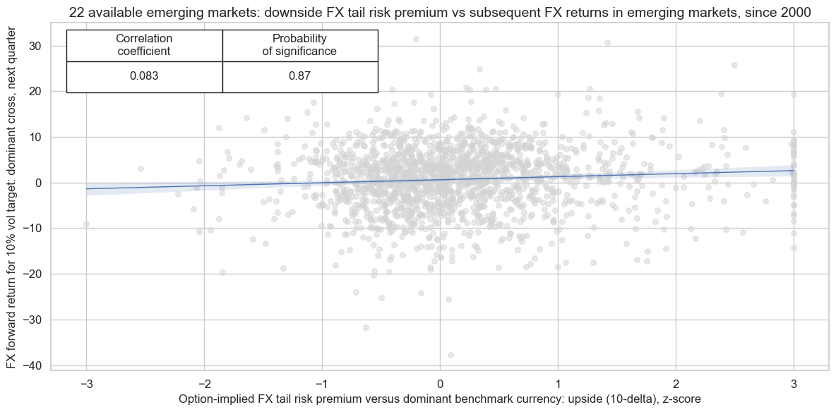
FX tail risk premia and subsequent FX forward returns #
There is some evidence that downside risk premia have positive predictive power for subsequent FX returns in emerging markets, suggesting that investors have, on balance, been compensated for bearing such risks. The predictive relationship is also positive in developed markets, however it fails to reach significance accordint to rigorous Macrosynergy panel test.
# Define signal and target mappings
sigx = {"FXPPTAILDOWN_NSAPZ": "Option-implied FX tail risk premium versus dominant benchmark currency: upside (10-delta), z-score"}

targx = {"FXXR_VT10": "FX forward return for 10% vol target: dominant cross"}

# Get common cross-section identifiers
cidx = msm.common_cids(dfx, xcats=list(sigx.keys()) + list(targx.keys()))
cidx = set(cids_em) & set(cidx)

cr = msp.CategoryRelations(
            dfx,
            xcats=[list(sigx.keys())[0], list(targx.keys())[0]],  # Assign correct signals & targets
            cids=cidx,  # Use the corresponding cross-sections for this market
            freq="Q",
            lag=1,
            xcat_aggs=["last", "sum"],
            blacklist=fxblack ,
            start="2000-01-01",
        )

cr.reg_scatter(
    prob_est = "map",
    xlab = f"{list(sigx.values())[0]}",
    coef_box="upper left",
    ylab = f"{list(targx.values())[0]}, next quarter",
    size = (12, 6),
    title=f"{len(cidx)} available emerging markets: downside FX tail risk premium vs subsequent FX returns in emerging markets, since 2000" ,)
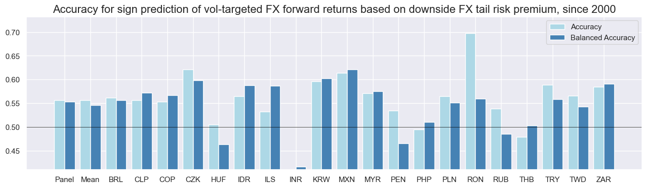
In emerging markets, the accuracy of predicting the sign of FX forward returns using normalized downside FX tail risk premia is well above 50% for majority of countries.
xcatx = ["FXPPTAILDOWN_NSAPZ", "FXXR_VT10"]
cidx = cids_exp

sr = mss.SignalReturnRelations(
    dfx,
    rets=xcatx[1],
    sigs=xcatx[0],
    agg_sigs="mean",
    cids=cids_em,
    blacklist=fxblack,
    freqs="Q",
    cosp=True,
)
sr.accuracy_bars(size = (16, 4),
                 title = "Accuracy for sign prediction of vol-targeted FX forward returns based on downside FX tail risk premium, since 2000",
                 )
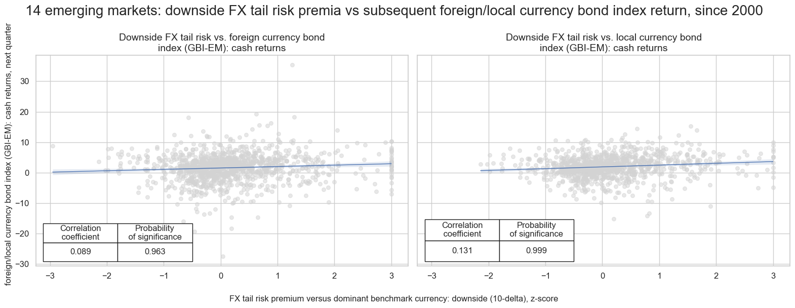
FX tail risk premium and subsequent emerging markets bond index returns #
FX tail risk premia seem to have significant positive power for emerging markets bond index returns, for both local-currency and foreign-currency indices. The predictive power has been more significant with respect to local-currency markets. High FX tail risk premia typically translate into elevated risk premia on local bond exposure.
# Define signal and target mappings
sigx = {
    "FXPPTAILDOWNUSD_NSAPZ": "FX tail risk premium versus dominant benchmark currency: downside (10-delta), z-score",
      }

targx = {
    "FCBIR_NSA": "foreign currency bond index (GBI-EM): cash returns",
    "LCBIR_NSA": "local currency bond index (GBI-EM): cash returns",
  }

# Define cross-section (market) groups
cidx = msm.common_cids(dfx, xcats=list(sigx.keys()) + list(targx.keys()))
cidx = list(set(cidx) & set(cids_em))

# Dictionary to store CategoryRelations objects
cr = {}

# Iterate through markets and matched signals/targets

for targ_name in targx.keys():
        cr[f"cr_{targ_name}"] = msp.CategoryRelations(
                dfx,
                xcats=[list(sigx.keys())[0], targ_name],
                cids=list(cidx),
                freq="Q",
                lag=1,
                xcat_aggs=["last", "sum"],
                blacklist=fxblack,
                start="2000-01-01",
            )

# Store all CategoryRelations instances in a list
all_cr_instances = list(cr.values())

subplot_titles = [
    f"Downside FX tail risk vs. {targx[targ_key]}"
    for targ_key in targx.keys()
]

vals = list(targx.values())
# Extract common suffix after the first space
common_suffix = vals[0].split(" ", 1)[1]  # "currency bond index (GBI-EM): cash returns"


# plot side by side all the CategoryRelations instances
msv.multiple_reg_scatter(
        all_cr_instances,
        title=f"{len(cidx)} emerging markets: downside FX tail risk premia vs subsequent foreign/local currency bond index return, since 2000" ,
        xlab=list(sigx.values())[0],
        ylab=f"foreign/local {common_suffix}, next quarter",
        ncol=2,
        nrow=1,
        figsize=(16, 6),
        prob_est="map",
        subplot_titles = subplot_titles,
        coef_box="lower left",
)
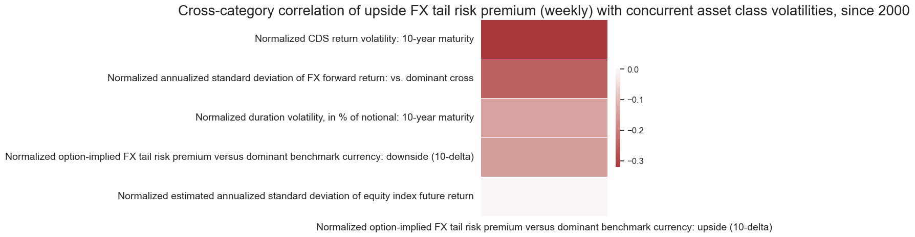
Correlation of FX tail risk premium with asset class volatilities #
FX tail risk premia (upside) are negatively correlated with the volatility of various asset classes—including CDS, equity indices, duration, and FX forward returns—as well as with downside tail risk premia, with all series expressed in z-scores. These inverse relationships are consistent across weekly, monthly, and quarterly frequencies and hold in both emerging and developed markets, except for a slightly positive correlation between FX tail risk premia and equity volatility in developed markets. The strongest negative correlation for upside FX tail risl premia is observed with sovereign CDS return volatility.
xcat_labels = {
    "FXPPTAILUP_NSAPZ": "Normalized option-implied FX tail risk premium versus dominant benchmark currency: upside (10-delta)",
   }
xcat_secondary_labels = {
    "CDS10YXRxEASD_NSAPZ": "Normalized CDS return volatility: 10-year maturity",
    "FXXRxEASD_NSAPZ": "Normalized annualized standard deviation of FX forward return: vs. dominant cross",
    "DU10YXRxEASD_NSAPZ": "Normalized duration volatility, in % of notional: 10-year maturity",
    "FXPPTAILDOWN_NSAPZ": "Normalized option-implied FX tail risk premium versus dominant benchmark currency: downside (10-delta)",
    "EQXRxEASD_NSAPZ": "Normalized estimated annualized standard deviation of equity index future return",
}

corr_df = msp.correl_matrix(
    dfx,
    xcats=list(xcat_labels.keys()),
    cids=cids_dmca+cids_em,
    title = "Cross-category correlation of upside FX tail risk premium (weekly) with concurrent asset class volatilities, since 2000" ,
    xcats_secondary=list(xcat_secondary_labels.keys()),
    freq="W",
    xcat_labels=xcat_labels,
    xcat_secondary_labels = list(xcat_secondary_labels.values()),
    size=(4, 5),
    cluster=False,
)
Appendices #
Appendix 1: Currency symbols #
The word ‘cross-section’ refers to currencies, currency areas or economic areas. In alphabetical order, these are AUD (Australian dollar), BRL (Brazilian real), CAD (Canadian dollar), CHF (Swiss franc), CLP (Chilean peso), CNY (Chinese yuan renminbi), COP (Colombian peso), CZK (Czech Republic koruna), DEM (German mark), ESP (Spanish peseta), EUR (Euro), FRF (French franc), GBP (British pound), HKD (Hong Kong dollar), HUF (Hungarian forint), IDR (Indonesian rupiah), ITL (Italian lira), JPY (Japanese yen), KRW (Korean won), MXN (Mexican peso), MYR (Malaysian ringgit), NLG (Dutch guilder), NOK (Norwegian krone), NZD (New Zealand dollar), PEN (Peruvian sol), PHP (Phillipine peso), PLN (Polish zloty), RON (Romanian leu), RUB (Russian ruble), SEK (Swedish krona), SGD (Singaporean dollar), THB (Thai baht), TRY (Turkish lira), TWD (Taiwanese dollar), USD (U.S. dollar), ZAR (South African rand).